ISSN 0101-8205 / ISSN 1807-0302 (Online) www.scielo.br/cam
Wavelet Galerkin method for solving singular
integral equations
K. MALEKNEJAD∗, M. NOSRATI and E. NAJAFI School of Mathematics, Iran University of Science & Technology Narmak
Tehran 16846, 13114, Iran
E-mails: [email protected] / [email protected] / [email protected]
Abstract. An effective technique upon linear B-spline wavelets has been developed for solving weakly singular Fredholm integral equations. Properties of these wavelets and some operational matrices are first presented. These properties are then used to reduce the computation of integral equations to some algebraic equations. The method is computationally attractive, and applications are demonstrated through illustrative examples.
Mathematical subject classification: 45A05, 32A55, 34A25, 65T60.
Key words:integral equation, weakly singular, operational matrices, linear B-spline wavelets, thresholding parameter.
1 Introduction
The aim of this study is to present a high order computational method for solving a special case of singular Fredholm integral equations of the second kind namely Abel’s integral equation defined as follows:
y(x)= f(x)−
Z b
a
K(x,t)|x−t|−αy(t)dt, (1)
0< α <1, a≤ x ≤b,
where f(x)andK(x,t)are known functions andy(x)is the unknown function that to be determined.
Abel’s equation is one of the integral equations derived directly from a con-crete problem of mechanics or physics (without passing through a differential equation). Historically, Abel’s problem is the first one that led to the study of integral equations. The generalized Abel’s integral equations on a finite segment appeared in the paper of Zeilon [1] for the first time.
A comprehensive reference on Abel-type equations, including an extensive list of applications, can be found in [2]-[5].
The construction of high order methods for the equations is, however, not an easy task because of the singularity in the weakly singular kernel. In fact, in this case the solution y is generally not differentiable at the endpoints of the interval [6]-[9], and due to this, to the best of the authors’ knowledge the best convergence rate ever achieved remains only at polynomial order. For example, if we set uniform meshes withn+1 grid points and apply the spline method so for orderm, then the convergence rate is only O(n−2P)at most [10]-[11], and it can not be improved by increasingm. One way of remedying this is to intro-duce graded meshes [10]-[12]. Then the rate is improved toO(n−m)[12] which now depends on m, but still at polynomial order. Fettis [13] proposed a numeri-cal form of the solution to Abel equation by using the Gauss-Jacobi quadrature rule. Piessens and Verbaeten [14] and Piessens [15] developed an approximate solution to Abel equation by means of the Chebyshev polynomials of the first kind. Numerical solutions of weakly singular Volterra integral equations were introduced in [16]-[21]. Yanzhao et al. [22] applied hybrid collocation methods for solving these equations. Rashit Ishik [23] used Bernstein series solution for solving linear integro-differential equations with weakly singular kernels. In [24] wavelet method is applied to solve noisy Abel-type equations. Wazwaz [25] studied on singular initial value problems in the second-order ordinary dif-ferential equations.
An algorithm for solving nonlinear singular perturbation problems is dis-cussed in [26].
In this work we assume that the K(x,t) ∈ [a,b] × [a,b] and satisfies in Lipschitz condition, that is:
|K(x1,t)−K(x2,t)| ≤Ls|x1−x2|, (2)
B-spline wavelets for solving weakly singular integral equations. Our method consists of reducing the given weakly singular integral equation to a set of alge-braic equations by expanding the unknown function by B-spline wavelets with unknown coefficients. Galerkin method is utilized to evaluate the unknown co-efficients. Because of semiorthogonality, compact support and having vanishing moments properties of these wavelets, the operational matrix is very sparse. Without loss of generality, we may consider[a,b] = [0,1].
The structure of this paper is arranged as follows. The main problem and brief history of some presented methods are expressed in Introduction 1. Linear B-spline scaling and wavelet functions on bounded interval are introduced in Section 2. Section 3 is devoted to function approximation by using B-spline wavelets and respective theorems. In Section 4, linear B-spline wavelets are ap-plied as testing and weighting functions of Galerkin method for efficient solution of equation 1. In Section 5 sparsity of the operational matrix and thresholding parameter is discussed. In Section 6, we report our numerical founds and com-pare them with other methods in solving these integral equations, and Section 7 contains our conclusion.
2 Linear B-spline scaling and wavelet functions
Basic definitions and concepts of wavelets is given in [27]-[33].
Definition 2.1.Let m and n be two positive integers and
c=x−m+1= ∙ ∙ ∙ =x0<x1<∙ ∙ ∙<xn =xn+1= ∙ ∙ ∙ =xn+m−1=d, be an equally spaced knots sequence. The functions
Bm,j,X(x)=
x −xj xj+m−1−xj
Bm−1,j,X(x)+
xj+m−x xj+m−xj+1
Bm−1,j+1,X(x), j = −m+1, . . . ,n−1,
and
B1,j,X(x)= (
1 x ∈ [xj,xj+1),
0 O.W.
For the sake of simplicity, suppose[c,d] = [0,n]andxk =k,k =0, . . . ,n. The Bm,j,X = Bm(x − j),j = 0, . . . ,n−m, are interior B-spline functions, while the remainingBm,j,X, j= −m+1, . . . ,−1 and j=n−m+1, . . . ,n−1 are boundary B-spline functions, for the bounded interval [0,n]. Since the boundary B-spline functions at 0 are symmetric reflections of those atn, it is sufficient to construct only the first half functions by simply replacing x with n−x.
By considering the interval[c,d] = [0,1], at any level j ∈ Z+, the
discretiza-tion step is 2−j, and this generatesn
= 2j number of segments in
[0,1]with knots sequence
X(j)=
x−(jm)+1= ∙ ∙ ∙ =x0(j)=0,
xk(j)= 2kj k =1, . . . ,n−1,
xn(j)= ∙ ∙ ∙ =xn(+j)m−1=1.
Let j0 be the level for which 2j0 ≥ 2m−1; for each level j ≥ j0the scaling functions of ordermcan be defined as follows in [33]:
ϕm,j,i(x)=
Bm,j0,i(2
j−j0x) i= −m+1, . . . ,−1,
Bm,j0,2j−m−i(1−2
j−j0x) i=2j −m+1, . . . ,2j −1,
Bm,j0,0(2
j−j0x−2−j0i) i=0, . . . ,2j −m,
(3)
and the two-scale relation for them-order semiorthogonal compactly supported B-wavelet functions are defined as follows:
ψm,j,i−m =
2i+X2m−2 k=i
qi,kBm,j,k−m, i =1, . . . ,m−1, (4)
ψm,j,i−m =
2i+X2m−2 k=2i−m
qi,kBm,j,k−m, i =m, . . . ,n−m+1, (5)
ψm,j,i−m =
n+Xi+m−1 k=2i−m
qi,kBm,j,k−m, i=n−m+2, . . . ,n, (6)
Hence, there are 2(m−1)boundary wavelets and(n−2m+2)inner wavelets in the boundary interval[c,d]. Finally by considering the level jwith j ≥ j0, the B-wavelet functions in[0,1]can be expressed as follows:
ψm,j,i(x)=
ψm,j0,i(2
j−j0x) i= −m+1, . . . ,−1
ψm,2j−2m+1−i,i(1−2j−j0x) i=2j −2m+2, . . . ,2j −m
ψm,j0,0(2
j−j0x−2−j0i) i=0, . . . ,2j−2m+1
(7)
The scaling functionsϕm,j,i(x), occupy msegments and the wavelet functions ψm,j,i(x)occupy 2m−1 segments.
Therefore the condition 2j ≥2m−1, must be satisfied in order to have at least one inner wavelet. In the following, the scaling functions and wavelet functions used in the paper, for j0= j=2 andm=2, are reported in [35]:
Boundary scalings
ϕ2,−1=1−4x, x ∈
0,1 4
(8)
ϕ2,3=4x−3, x ∈
3
4,1
(9)
Inner scalings
ϕ2,0(x)= (
4x, x ∈0,14
2−4x, x ∈14,12 (10)
ϕ2,1(x)= (
4x −1, x ∈14,12
3−4x, x ∈12,34 (11)
ϕ2,2(x)= (
4x −2, x ∈12,34
4−4x, x ∈34,1 (12)
Boundary wavelets
ψ2,−1=
−1+463x, x ∈0,18 7
3 − 34
3x, x ∈
1 8, 1 4 −5 3 + 14
3x, x ∈
1 4, 3 8 1 3 − 2
3x, x ∈
ψ2,2= −1 3 + 2
3x, x ∈
1 2,
5 8
3−143x, x ∈58,34
−9+343x, x ∈34,78 43
3 − 46
3x, x ∈
7 8,1
(14)
Inner wavelets
ψ2,0=
2
3x, x ∈ [0,
1 8) 2
3− 14
3x, x ∈
1 8, 1 4 −19 6 + 32
3x, x ∈
1 4, 3 8 29 6 − 32
3x, x ∈
3 8, 1 2 −17 6 + 14
3x, x ∈
1 2, 5 8 1 2− 2
3x, x ∈
5 8, 3 4 (15)
ψ2,1=
−1 12 + 2
3x, x ∈
1 8, 1 4 5 4− 14
3x, x ∈
1 4, 3 8 −9 2 + 32
3x, x ∈
3 8, 1 2 37 6 − 32
3x, x ∈
1 2, 5 8 −41 12 + 14
3x, x ∈
5 8, 3 4 7 12− 2
3x. x ∈
3 4, 7 8 (16)
Some of the important properties relevant to the present work are given below:
1) Vanishing moments: A waveletψ(x)is said to have a vanishing moments of ordermif
Z ∞
−∞
xpψ (x)d x =0; p=0,1, . . . ,m−1.
All wavelets must satisfy the above condition for p=0. Linear B-spline wavelet has 2 vanishing moments. That is
Z ∞
−∞
xpψ4(x)d x =0, p=0,1.
2) Semiorthogonality: The waveletsψj,kform a semiorthogonal basis if
hψj,k, ψs,ii =0, j6=s, ∀j,k,s,i ∈Z.
Linear B-spline wavelet are semiorthogonal.
3 Function approximation
A function f(x)defined over[0,1]may be approximated by B-spline wavelets as [34]:
f(x)= 2Xj0−1
i=−1
cj0,iϕj0,i(x)+
∞ X
j=j0 2j−2
X
k=−1
dj,kψj,k(x), (17)
where ϕj0,i and ψj,k are scaling and wavelets functions, respectively. If the infinite series in equation 17 is truncated, then it can be written as:
f(x)≃ 2Xj0−1 i=−1
cj0,iϕj0,i(x)+ ju X
j=j0 2j−2
X
k=−1
dj,kψj,k(x)=CT9(x), (18)
whereCand9are 2(ju+1)+1 column vectors given by:
C=cj0,−1, . . . ,cj
0,2j0−1,dj0,−1, . . . ,dj0,2j0−2, . . . ,dju,−1, . . . ,dju,2ju−2 T
, (19)
9=ϕj0,−1, . . . , ϕj0,2j0−1, ψj0,−1, . . . , ψj0,2j0−2, . . . , ψju,−1, . . . , ψju,2ju−2 T
, (20)
with
cj0,i =
Z 1
0
f(x)ϕ˜j0,i(x)d x, i= −1, . . . ,2 j0
−1, (21)
dj,k =
Z 1
0
f(x)ψj˜ ,k(x)d x, j = j0, . . . , ju, k = −1, . . . ,2ju −2, (22)
whereϕ˜j0,iandψ˜j,kare dual functions ofϕj0,i,i = −1, . . . ,2
j0−1 andψj
,k, j =
j0, . . . , ju, respectively. These can be obtained by linear combinations ofϕj0,i andψj,k.
Theorem 3.1. We assume that f ∈ C2[0,1]is represented by linear B-spline wavelets as equation 18, whereψhas 2 vanishing moments, then
|dj,k| ≤αβ 2−3k
whereα = max|f(2)(t)
|,t ∈ [0,1]andβ = R01t2ψ (t)dt. Moreover if ee j(x) be the approximation error in the subspace Vj, then:
|ej(x)| =O(2−2j).
Proof. ([35])
4 Description of the numerical method
In this section, we solve the singular integral equation of the form 1 by using B-spline wavelets. For this purpose the unknown function of the equation 1 is expanded by linear B-spline wavelets as equation 18. The integral term in equation 1 can be written as:
Z 1
0
K(x,t)|x −t|−αy(t)dt =
Z 1
0
(K(x,t)−K(x,x))|x−t|−αy(t)dt
+K(x,x)
Z 1
0 |
x −t|−αy(t)dt,
and
Z 1
0 |
x−t|−αy(t)dt =
Z 1
0 |
x −t|−α(y(t)−y(x))dt
+ y(x)
Z 1
0
|x−t|−αdt,
thus we have
Z 1
0
(K(x,t)−K(x,x))|x−t|−αy(t)dt
≤
Z 1
0 |
K(x,t)−K(x,x)| |x−t|−α|y(t)|dt
≤
Z 1
0
Ls|x −t|1−α|y(t)|dt, now asx →t,
Z 1
0
(K(x,t)−K(x,x))|x−t|−αy(t)dt
On the other hand
Z 1
0 |
x −t|−α(y(t)−y(x))dt
≤
Z 1
0 |
x−t|−α|y(t)−y(x)|dt
≤ y′(ξ )
Z 1
0 |
x −t|1−αdt
= y′(ξ )|x−t| 2−α
2−α ,
so, asx →t
Z 1
0
(x −t)−α(y(t)−y(x))dt
→0. (24)
Now we introduce the functionH(x,t)as:
H(x,t)=
(
K(x,t)(x −t)−α x 6=t
0 x =t. (25)
So the integral term of equation 1 can be written as:
Z 1
0
K(x,t)(x−t)−αy(t)dt =
Z 1
0
H(x,t)y(t)dt, (26)
and we note that the new kernel function is not singular in [0,1]. Thus the integral equation 1 can be rewritten as follows:
y(x)= f(x)+
Z 1
0
H(x,t)y(t)dt. (27)
Substituting function approximation 18 in current equation and employing Galerkin method, the following set of linear system of order 2ju +1 is
gen-erated. Linear B-spline scaling and wavelet functions are used in testing and weighting functions of Galerkin method.
hHφ, φi − hφ, φi hHψ, φi − hψ, φi
hHφ, ψi − hφ, ψi hHψ, ψi − hψ, ψi
!
× C
D
!
= F1
F2
!
(28)
where
C = cj0,−1, . . . ,cj0,2j0−1
T
, (29)
D= dj0,−1, . . . ,dj0,2j0−2, . . . ,dju,−1, . . . ,dju,2ju−2 T
hHφ, φi − hφ, φi =
Z 1
0
ϕj0,r(x)
Z 1
0
H(x,t)ϕj0,i(t)dtd x
−
Z 1
0
ϕj0,r(x)ϕj0,i(x)d x
i,r ,
(31)
hHψ, φi − hψ, φi =
Z 1
0
ϕj0,r(x)
Z 1
0
H(x,t)ψj,k(t)dtd x
−
Z 1
0
ϕj0,r(x)ψj,k(x)d x
r,k,j ,
(32)
hHφ, ψi − hφ, ψi =
Z 1
0
ψs,l(x)
Z 1
0
H(x,t)ϕj0,i(t)dtd x
−
Z 1
0
ψs,l(x)ϕj0,i(x)d x
i,l,s ,
(33)
hHψ, ψi − hψ, ψi =
Z 1
0
ψs,l(x)
Z 1
0
H(x,t)ψj,k(t)dtd x
−
Z 1
0
ψs,l(x)ψj,k(x)d x
l,s,k,j ,
(34)
F1=
Z 1
0
f(x)ϕj0,r(x)d x, (35)
F2=
Z 1
0
f(x)ψs,l(x)d x, (36)
And the subscriptsi,r,k, j,lands assume values as given below:
i,r = −1, . . . ,2j0−1, s,j = j0, . . . , ju,
l,k = −1, . . . ,2ju −2.
It can be shown that the total number of unknowns in 28, does not depend on j0as given below:
N =2ju
+1. (37)
zero due to the semi orthogonality and vanishing moments properties of the wavelet functions.
In fact the entries with significant magnitude are in thehHφ, φi − hφ, φiand
hHψ, ψi − hψ, ψisub matrices which are of order (2j0 +1)and(2ju+1+1)
respectively.
5 Matrix sparsity and thresholding error
Because of the local supports and vanishing moments properties of B-spline wavelets, many of the matrix elements in equation 18 are very small compared to the largest element, and hence we can set to zero with an opportune threshold technique without significantly affecting the solution. Typically one thresholds the elements of a wavelet matrix by setting to zero all elements that are less than some small positive number multiplied by the largest matrix element, we show byδ. The matrix sparsitySδdefined by
Sδ =
Ne−Nδ
Ne ×100,
where Ne is the total number of elements and Nδ is the number of nonzero
elements remaining after thresholding. The relative error caused by thresholding the wavelet matrix is defined by
ε = kfe− fδk2
kfek2 ×
100.
6 Illustrative examples
Example 1. Consider the singular integral equation [36]
y(x)= f(x)+
Z 1
0 1
10|x−t|
−1/3y(t)dt,
with
f(x)=x2(1−x)2− 27
30800
× x8/3(54x2
−126x+77)+(1−x)8/3(54x2
+18x +5).
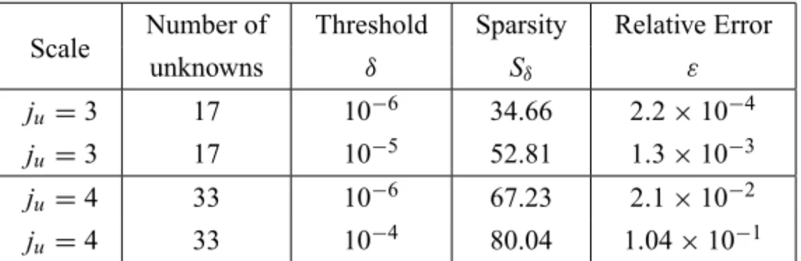
The exact solution y(x) = x2(1−x)2. The solution for y(x) is obtained by the method in Section 4 at the octave level j0 =2 and at the levels ju =3 and 4. The results without thresholding and for different thresholding parameters and diverse scales are shown in Tables 1 and 2. In Table 1, we present exact and approximate solutions of Example 1 in some arbitrary points. As proved in Theorem 1, the error at the level ju =4 is smaller than the error at ju =3, moreover errors in our method are smaller than those in other methods. More-over, because of semiorthogonality and having vanishing moments of B-spline wavelets, matrices in our method are sparse, thus we do not need large memory requirement and a high computational time.
Approximate Approximate S.C.M.* x
ju=3 ju =4 [36] Exact
0 0 0 0 0
0.1 0.008103 0.0081000 0.00812 0.0081 0.2 0.025604 0.0256000 0.02565 0.0256 0.3 0.044101 0.0441000 0.04414 0.0441 0.4 0.057609 0.0576000 0.05768 0.0576 0.5 0.062503 0.0625000 0.06259 0.0625 0.6 0.057608 0.0576000 0.05763 0.0576 0.7 0.044102 0.0441000 0.04414 0.0441 0.8 0.025606 0.0256000 0.02563 0.0256 0.9 0.008104 0.0081000 0.00816 0.0081
1 0 0 0 0
Number of Threshold Sparsity Relative Error Scale
unknowns δ Sδ ε
ju=3 17 10−6 34.66 2.2×10⁻⁴
ju=3 17 10−5 52.81 1.3×10⁻³
ju=4 33 10−6 67.23 2.1×10⁻²
ju=4 33 10−4 80.04 1.04×10⁻¹
Table 2 – Sparsity and relative error for wavelet matrices of Example 1 in different scales and threshold parameters.
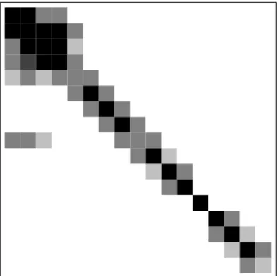
Figure 1 shows the grayscale plot of the matrix obtained by setting the thresh-old to 10−5at the level ju =3. Table 2 shows a comparison of sparsity and rela-tive error for semi orthogonal B-spline wavelets in different scales and threshold parameter. It is interesting that at the scale ju = 4 with threshold parameter 10−4, the number of matrix element 1089 decrease to 262.
Figure 1 – Grayscale plot of the magnitude of the wavelet matrix elements for Example 1
at the octave level j0=2 for the threshold parameter 10−5at the level ju=3.
Example 2. Consider the problem [10], [11] 3√2
4 y(x)−
Z 1
0 |
x −t|−1/2y(t)dt =3
x(1−x)3/4−3
8π(1+4x(1−x))
with the exact solution 2√2(x(1− x))3/4. The solution for y(x) is obtained by the method in Section 4 at the octave level j0=2 and at the levels ju =3 and 4. The results without thresholding and for different thresholding parameters and diverse scales are shown in Tables 3 and 4. Figure 2 shows the grayscale plot of the matrix obtained by setting the threshold to 10−4at the level ju=4.
Approximate Approximate P.I.M.* x
ju=3 ju =4 [37]
Exact
0 0 0 0 0
0.1 0.464756 0.46475804 0.464768 0.464758 0.2 0.715541 0.71554201 0.715548 0.715542 0.3 0.877428 0.87742402 0.877418 0.877424 0.4 0.969845 0.96984702 0.969862 0.969847
0.5 1.00001 1.000000 1.000037 1
0.6 0.969844 0.96984703 0.96984749 0.969847 0.7 0.877423 0.87742400 0.877463 0.877424 0.8 0.715545 0.71554201 0.715527 0.715542 0.9 0.464754 0.46475803 0.464734 0.464758
1 0 0 0 0
Table 3 – Exact and approximate solutions of Example 2 without thresholding. ∗P.I.M: Product Integration Method.
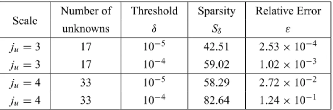
Number of Threshold Sparsity Relative Error Scale
unknowns δ Sδ ε
ju=3 17 10−5 42.51 2.53×10⁻⁴
ju=3 17 10−4 59.02 1.02×10⁻³
ju=4 33 10−5 58.29 2.72×10⁻²
ju=4 33 10−4 82.64 1.24×10⁻¹
Table 4 – Sparsity and relative error for wavelet matrices of Example 2 in different scales and threshold parameters.
7 Conclusions
Figure 2 – Grayscale plot of the magnitude of the wavelet matrix elements for Example 2
at the octave level j0=2 for the threshold parameter 10−4at the level ju=4.
compactly supported spline wavelets. The wavelet MOM used via the Galerkin procedure. Based on the consideration reported in figures and tables, the method presented in this paper determines a strong reduction of the computation time and memory requirement in inverting the matrix. The approach can be extended to nonlinear singular integral and integro-differential equations with little addi-tional work. Further research along these lines is under progress and will be reported in due time.
REFERENCES
[1] N. Zeilon, Sur quelques points de la theorie de l’equation integrale d’Abel.Arkiv. Mat. Astr. Fysik.,18(1924), 1–19.
[2] R. Gorenflo and S. Vessella, Abel Integral Equations.Lecture Notes in Mathe-matics, vol. 1461, Springer, Berlin (1991).
[3] J.J. Nieto and W. Okrasinski, Existence, uniqueness, and approximation of solu-tions to some nonlinear diffusion problems.J. Math. Anal. Appl.,210(1) (1997), 231–240.
[5] R. Gorenflo and S. Vessella, Abel Integral Equations: Analysis and Applications. Springer-Verlag, Berlin (1991).
[6] C. Schneider, Regularity of the solution to a class of weakly singular Fredholm integral equations of the second kind.Integral Equation Operator Theory,2(1979), 62–68.
[7] G.R. Ritcher,On weakly singular Fredholm integral equations with displacement kernels.J. Math. Anal. Appl.,55(1976), 32–48.
[8] G. Vainikko and A. Pedas, The properties of solutions of weakly singular integral equations.J. Aust. Math. Soc. Ser. B,22(1981), 419–430.
[9] I.G. Graham, Singularity expansions for the solutions of second kind Fredholm integral equations with weakly singular convolution kernels.J. Integral Equations, 4(1982), 1–30.
[10] C. Schneider, Product integration for weakly singular integral equations.Math. Comput.,36(1981), 207–213.
[11] I.G. Graham,Galerkin methods for second kind integral equations with singular-ities.Math. Comput.,39(1982), 519–533.
[12] G. Vainikko and P. Uba, A piecewise polynomial approximation to the solution of an integral equation with weakly singular kernel.J. Austral. Math. Soc. Ser. B, 22(1981), 431–438.
[13] M.E. Fettis, On numerical solution of equations of the Abel type.Math. Comp., 18(1964), 491–496.
[14] R. Piessens and P. Verbaeten, Numerical solution of the Abel integral equation. BIT,13(1973), 451–457.
[15] R. Piessens,Computing integral transforms and solving integral equations using Chebyshev polynomial approximations.J. Comput. Appl. Math.,121(2000), 113– 124.
[16] S. Karimi and A. Aminataei, Operational Tau approximation for a general class of fractional integro-differential equations.Comput. Appl. Math.,30(2011), 655–674.
[17] A.M.A. El-Sayed, H.H.G. Hashem and E.A.A. Ziada,Picard and Adomian meth-ods for quadratic integral equation.Comput. Appl. Math.,29(2010), 447–463.
[19] P. Baratella and A.P. Orsi, A new approach to the numerical solution of weakly singular Volterra integral equations.J. Computat. Appl. Math.,163(2004), 401– 418.
[20] M.A. Abdou and A.A. Nasr, On the numerical treatment of the singular in-tegral equation of the second kind. Applied Mathematics and Computation, 146(2-3) (2003), 373–380.
[21] M.A. Darwish, Weakly singular functional-integral equation in infinite dimen-sional Banach spaces. Applied Mathematics and Computation, 136(1) (2003), 123–129.
[22] C. Yanzhao, H. Min, L. Liping and X. Yuesheng, Hybrid collocation methods for Fredholm integral equations with weakly singular kernels.Applied Numerical Mathematics,57(5-7) (2007), 549–561.
[23] O. Rasit Isik, M. Sezer and Z. Güney,Bernstein series solution of a class of linear integro-differential equations with weakly singular kernel.Applied Mathematics and Computation,217(16) (2011), 7009–7020.
[24] P. Hall, R. Paige and F.H. Ruymagaart, Using wavelet methods to solve noisy Abel-type equations with discontinuous inputs.J. Multivariate. Anal.,86(2003), 72–96.
[25] A.M. Wazwaz, A new method for solving singular initial value problems in the second-order ordinary differential equations.Applied Mathematics and Compu-tation,128(1) (2002), 45–57.
[26] W. Weiming, An algorithm for solving nonlinear singular perturbation prob-lems with mechanization.Applied Mathematics and Computation,169(2) (2005), 995–1009.
[27] C. Chui, An introduction to wavelets. New York: Academic Press (1992).
[28] I. Daubechies, Ten lectures on wavelets. Philadelpia, PA: SIAM (1992).
[29] G. Strang and T. Nguyen, Wavelets and filter banks. Cambridge, MA: Wellesley-Cambridge (1997).
[30] L. Telesca, G. Hloupis, I. Nikolintaga and F. Vallianatos, Temporal patterns in southern Aegean seismicity revealed by the multiresolution wavelet analysis. Commun. Nonlinear Sci. Num. Simul.,12(2007), 1418–1426.
[32] K. Maleknejad, K. Nouri and M. Nosrati Sahlan, Convergence of approximate solution of nonlinear Fredholm-Hammerstein integral equations.Communication in Nonlinear Science and Numerical Simulation,15(6) (2010), 1432–1443.
[33] G. Ala, M.L. Silvestre, E. Francomano and A. Tortorici,An advanced numerical model in solving thin-wire integral equations by using semiorthogonal compactly supported spline wavelets.IEEE Trans. Electromagn. Compact,45(2003), 218– 228.
[34] M. Lakestani, M. Razzaghi and M. Dehghan, Solutions of nonlinear Fredholm-Hamerstein integral equations by using semiorthogonal spline wavelets. Math. Prob. Eng.,1(2005), 113–121.
[35] K. Maleknejad and M. Nosrati Sahlan, The method of moments for solution of second kind Fredholm integral equations based on B-spline wavelets.International Journal of Computer Mathematics,87(2010), 1602–1616.
[36] T. Okayama, T. Matsuo and M. Sugihara, Sinc-collocation methods for weakly singular Fredholm integral equation of the second kind.J. Comput. Appl. Math., 234(2010), 1211–1227.