Numerical Solution of Second-Order Linear Fredholm Integro-Differential Equation Using Generalized Minimal Residual Method

American Journal of Applied Sciences 7 (6): 780-783, 2010 ISSN 1546-9239

© 2010Science Publications

Corresponding Author: Elayaraja Aruchunan, Department of Engineering and Science, School of Foundation and Continuous Studies, Curtin University of Technology, CDT 250, 98009 Miri, Sarawak, Malaysia

780

Numerical Solution of Second-Order Linear Fredholm Integro-Differential Equation

Using Generalized Minimal Residual Method

1

Elayaraja Aruchunan and

2

Jumat Sulaiman

1

Department of Engineering and Science, School of Foundation and Continuous Studies,

Curtin University of Technology, CDT 250, 98009 Miri, Sarawak Malaysia

2

Mathematics with Economics Programme, University Malaysia Sabah, Locked Bag 2073,

88999 Kota Kinabalu, Sabah, Malaysia

Abstract: Problem statement: This research purposely brought up to solve complicated equations such as partial differential equations, integral equations, Integro-Differential Equations (IDE), stochastic equations and others. Many physical phenomena contain mathematical formulations such integro-differential equations which are arise in fluid dynamics, biological models and chemical kinetics. In fact, several formulations and numerical solutions of the linear Fredholm integro-differential equation of second order currently have been proposed. This study presented the numerical solution of the linear Fredholm integro-differential equation of second order discretized by using finite difference and trapezoidal methods. Approach: The linear Fredholm integro-differential equation of second order will be discretized by using finite difference and trapezoidal methods in order to derive an approximation equation. Later this approximation equation will be used to generate a dense linear system and solved by using the Generalized Minimal Residual (GMRES) method. Results: Several numerical experiments were conducted to examine the efficiency of GMRES method for solving linear system generated from the discretization of linear Fredholm integro-differential equation. For the comparison purpose, there are three parameters such as number of iterations, computational time and absolute error will be considered. Based on observation of numerical results, it can be seen that the number of iterations and computational time of GMRES have declined much faster than Gauss-Seidel (GS) method. Conclusion: The efficiency of GMRES based on the proposed discretization is superior as compared to GS iterative method.

Key words: Fredholm integro-differential, finite difference, quadrature, generalized minimal residual

INTRODUCTION

Integro-Differential Equation (IDE) is an important branch of modern mathematics and arises frequently in many applied areas which include engineering, mechanics, physics, chemistry, astronomy, biology, economics, potential theory and electrostatics (Kurt and Sezer, 2008). IDE is an equation that the unknown function appears under the sign of integration and it also contains the derivatives of the unknown function. It can be classified into Fredholm equations and Volterra equations. The upper bound of the region for integral part of Volterra type is variable, while it is a fixed number for that of Fredholm type. In this study, we focus on second order linear Fredholm integro-differential equation. Generally, second-order linear

Fredholm integro-differential equations can be defined as follows:

( )

( ) ( )

( )

b a

p x y ''(x) q(x)y '(x) r(x)y(x)

k x, t y t dt f x

+ + +

=

∫

(1)

with initial conditions:

y(0)=m, y'(0)=n Where, the functions:

p(x), q(x), r(x) = Constant matrices

f(x) = A given vector function, the kernel k(x,t) = A given matrix function

Am. J. Applied Sci., 7 (6): 780-783, 2010

781 In the engineering field, numerical approaches were practiced to obtain an approximation solution for the problem (1). To solve a linear integro-differential equation numerically, discretization of integral equation to the solution of system of linear algebraic equations is the basic concept used by researchers to solve integro-differential problems. By considering numerical techniques, there are many methods can be used to discretize problem (1) such as compact finite difference (Zhao and Corless, 2006), Wavelet-Galerkin (Avudainayagam and Vani, 2000), variational iteration method (Sweilam, 2007) rationalized Haar functions (Maleknejad et al., 2004), Tau, (Hosseini and Shahmorad, 2003), Lagrange interpolation (Rashed, 2003), piecewise approximate solution (Hosseini and Shahmorad, 2005), conjugate gradient (Khosla and Rubin, 1981), quadrature-difference (Fedotov, 2009), variational (Saad and Schultz, 1986), collocation (Aguilar and Brunner, 1988), homotopy perturbation (Yildirim, 2008) and Euler-Chebyshev method (Van der Houwen and Sommeijer, 1997). Earlier numerical treatment has been done for first order integro-differential equation (Aruchunan and Sulaiman, 2009).

In this conjunction, there are many iterative methods under the category of Krylov subspaces have been proposed widely to be one of the feasible and successful classes of numerical algorithms for solving linear systems. Actually, there are several Krylov subspaces iterative methods can be considered such as Conjugate Gradient (CG) (Hestenes and Stiefel, 1952), Generalized Minimal Residual (GMRES) (Saad and Schultz, 1986), Conjugate Gradient Squared (Sonneveld, 1989), Bi-Conjugate Gradient Stabilized (Bi-CGSTAB) (Van der Vorst, 1992) and Orthogonal Minimization (ORTHOMIN) (Vinsome, 1976).

In this study, GMRES iterative method will be used for solving linear algebraic equations produced by the discretization of the second-order linear Fredholm integro-differential equations by using quadrature and finite difference methods. For differential part, second order central difference scheme was used for approximation whereas the integral term was discretized by quadrature method. In order to compare the efficiency of the GMRES method, Gauss-Seidel (GS) method was used for numerical comparison.

MATERIALS AND METHODS

Approximation equation: As afore-mentioned, a discretization method based on quadrature and finite difference methods was used to construct approximation equations for problem (1).

Quadrature method: The formulas of quadrature method, in general have the form:

n b

j j n a

j 0

y(t)dt A y(t ) (y)

=

=

∑

+ ε

∫

(2)

where, t ( jj =0,1,…, n) are the abscissas of the partition points of the integration interval [a,b] or quadrature (interpolation) nodes, Aj (j = 0,1,…,n) are numerical

coefficients that do not depend on the function y(t) and

εn(y) is the truncation error of Eq. 2. To facilitate in

formulating the approximation equations for problem (1), further discussion will restrict onto Repeated Trapezoidal (RT) method, which is based on linear interpolation formulas with equally spaced data. Based on RT method, numerical coefficients Aj are satisfied

the following relation:

j 1

h, j 0, n

A 2

h, j 1, 2, , n 1

 ₌



=

 _{= −}

 ⋯

(3)

where, the constant step size, h is defined as: b a

h n −

= (4)

n is the number of subintervals in the interval [a,b]. Finite difference method: In this study, second order central difference approximation formulas were used as follow:

i 1 i 1 i

dy y y

dx 2h

+ − −

≅ (5a)

2

i 1 i i 1

2 2

i

d y y 2y y

dx h

+ − + −

≅ (5b)

where, y′

( )

x_i and y′′

( )

x_i are approximated by second order finite difference schemes. By applying Eq. 2 and 5 into Eq. 1, a system of linear algebraic equations obtains for approximation values y(x) at the nodes

0 1 n

x , x ,…, x _{. The generated linear systems can be easily} shown as:

~ ~

Am. J. Applied Sci., 7 (6): 780-783, 2010

782 In this study, interval [a,b] will be uniformly divided into m

n=2 , m≥2 and then consider the discrete set of points be given as xi= +a ih.

Generalized Minimal Residual (GMRES) method: The GMRES is an efficient algorithm for iteratively solving a general linear system in Eq. 4. The method is based upon the Arnoldi process (Saad and Schultz, 1986), which constructs an orthonormal basis of the Krylov subspace m

1

k (M; v ). The subspace is defined as:

m m 1

1 1 1 1

k (A; v )=span {v , Av ,…, A −v }

where, v1=r / r0 0 2, r0= −f Av }0 and x0 is the initial guess. The idea of GMRES is to find an approximation of x in which f−My₂ is minimal. The GMRES algorithm may be described in Algorithm 1 (Saad, 2003).

Algorithms 1: GMRES method:

Step 1 Start: Choose x0, computer0= −f Mx0; Step 2 For j = 1, 2… until convergence

02 1 0 1

r , v x / , p e ;

β = = β = β

Step 3 For, i=1, 2,…, m i

w=Av ; For, k=1, 2,…,i k ,i i

h = w, v ;

k ,i k i 1 2 i 1 i 1,i

k ,i

w w h v ;

h w ;

v w / h ;

H {h };

+

+ +

= − = = =

For k=2,…,i

k 1,i k 1 k 1,i k 1 k ,i h₋ =C₋h ₋ +S₋h ;

k ,i k 1 k 1,i k 1 k ,i 2 2

i,i i 1,i i i,i i i 1 i,i i i,i i i,i i 1 i i i i i

h S h C h ;

h h ;

C h / ,S h / ;

h C h S h / ;

p S p , p C p ;

− − −

+

+

+

= − +

γ = +

= γ = γ

= + γ

= − =

Step 4 If pi 1+ ≤ ε then

End for i

1 1,1 1, k 1

k k, k 2

y h h p

y 0 h p

 

   

 

   

= 

   

 

   

    

⋯

⋮ ⋮ ⋱ ⋮ ⋮

⋯

j 0 i i

i 1

x x y v

=

= +

∑

Step 5 Ifpi 1+ ≤ εend for j else x0=x

RESULTS AND DISCUSSION

In this conjunction, the GMRES method was tested with the following problem (Hosseini and Shahmorad, 2005) and then compared its performances with GS method:

( )

15 5 ''

0

e 1

y (x) 9y(x) y t dt

3 x [0,5]

− ₋

= + +

_∫

∈ (7)

( )

'

( )

y 0 =1, y 0 = −3, with the exact solution

( )

3x

y x =e− .

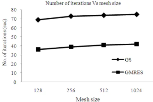
In this research, parameters such as number of iterations, execution time and absolute error are considered as comparison. Throughout the simulations, the convergence test considered the tolerance error of the

ε = 10−16. Figure 1 and 2 show number of iterations and execution time versus mesh size, respectively. Furthermore, the numerical results of this application presented with exact solution have been shown in Table 1.

Fig. 1: Comparison on the number of iterations for the GS and GMRES methods

Am. J. Applied Sci., 7 (6): 780-783, 2010

783 Table 1: Comparison of number of iterations, execution time and

maximum absolute error for the iterative methods Mesh size

---

Methods 128 256 512 1024

Number of iterations

GS 69 73 74 75

GMRES 36 39 41 42

Execution time (sec)

128 256 512 1024

GS 5.60 11.34 31.04 66.71

GMRES 3.03 6.89 18.88 37.54

Methods

Maximum absolute error

128 256 512 1024

GS 4.6987 E-2 3.3389 E-3 5.5060 E-3 9.8834 E-4 GMRES 4.0043 E-2 3.1170 E-3 5.3332 E-3 9.5621 E-4

CONCLUSION

Based on the results in Table 1, number of iterations of the GMRES methods has decreased approximately 44.00-47.82% compared to GS method as shown in Fig. 1. For the execution time, GMRES method is much faster about 39.17-45.85% compared to GS method, see in Fig. 2. As a conclusion, the numerical results have shown that the GMRES method is more advanced in term of number of iterations and the execution time than GS method.

REFERENCES

Aguilar, M. and H. Brunner, 1988. Collocation methods for second-order Volterra integro-differential equations. Applied Numer. Math., 4: 455-470. DOI: 10.1016/0168-9274(88)90009-8

Aruchunan, E. and J. Sulaiman, 2009. Numerical solution of first kind linear Fredholm Integro-differential equation using conjugate gradient method. Proceedings of the Curtin Sarawak 1st International Symposium on Geology, Sept. 2009, pp: 11-13.

Avudainayagam, A. and C. Vani, 2000. Wavelet- Galerkin method for integro-differential equations. Applied Math. Comput., 32: 247-254. DOI: 10.1016/S0168-9274(99)00026-4

Fedotov, A.I., 2009. Quadrature-difference methods for solving linear and nonlinear singular integro-differential equations. Nonlinear Anal., 71: 303-308. DOI: 10.1016/j.na.2008.10.075

Hestenes, M. and E. Stiefel, 1952. Methods of conjugate gradients for solving linear system. J. Res. Nat. Bur. Stand., 49: 409-436. http://nvl.nist.gov/pub/nistpubs/jres/049/6/V49.N06. A08.pdf

Hosseini, S.M. and S. Shahmorad, 2003. Tau numerical solution of Fredholm integro-differential equations with arbitrary polynomial bases. Applied Math. Model, 27: 145-154. DOI: 10.1016/S0307-904X(02)00099-9

Hosseini, S.M. and S. Shahmorad, 2005. Numerical piecewise approximate solution of Fredholm integro-differential equations by the Tau method. Applied Math. Model., 29: 1005-1021. DOI: 10.1016/j.apm.2005.02.003

Khosla, P.K. and S.G. Rubin, 1981. A conjugate gradient iterative method. Comput. Fluids, 9: 109-121. DOI: 10.1016/0045-7930(81)90020-7

Kurt, N. and M. Sezer, 2008. Polynomial solution of high-order Fredholm integro-differential equations with constant coefficients. J. Franklin Inst., 345: 839-850. DOI: 10.1016/j.jfranklin.2008.04.016 Maleknejad, K., F. Mirzaee and S. Abbasbandy, 2004. Solving linear integro-differential equations system by using rationalized Haar functions method. Applied Math. Comput., 155: 317-328. DOI: 10.1016/S0096-3003(03)00778-1

Rashed, M.T., 2003. Lagrange interpolation to compute the numerical solutions differential and integro-differential equations. Applied Math. Comput., 151: 869-878. DOI: 10.1016/S0096-3003(03)00543-5 Saad, Y. and M.H. Schultz, 1986. GMRES: A generalized minimal residual algorithm for solving non-symmetric linear sytems. SIAM J. Sci. Stat. Comput., 7: 856-869. DOI: 10.1137/0907058 Saad, Y., 2003. Iterative Methods for Sparse Linear

Systems. Society for Industrial and Applied Mathematics (SIAM). ISBN: 0898715342, pp: 158. Sonneveld, P., 1989. CGS A fast Lanczos-type solver

for nonsymmetric linear systems. SIAM J. Sci. Stat.Comput., 10: 36-52. DOI: 10.1137/0910004 Sweilam, N.H., 2007. Fourth order integro-differential

equations using variational iteration method. Comput. Math. Appli, 54: 1086-1091. DOI: 10.1016/j.camwa.2006.12.055

Van der Houwen, P.J. and B.P. Sommeijer, 1997. Euler-Chebyshe methods for integro-differential equations. Applied Numer. Math., 24: 203-218. DOI: 10.1016/S0168-9274(97)00021-4

Van der Vorst, H., 1992. Bi-CGSTAB: A fast and smoothly converging variant of Bi-CG for the solution of non-symmetric linear systems. SIAM J. Sci. Stat. Comput., 13: 631-644. DOI: 10.1137/0913035 Vinsome, P.K.W., 1976. ORTHOMIN, An iterative

method for solving sparse sets of simultaneous linear equations. Proceedings of SPE Symposium on Numerical Simulation of Reservoir Performance, Feb. 19-20, Los Angeles, California, pp: 5729. Yildirim, A., 2008. Solution of BVPs for fourth-order

integro differential equations by using homotopy perturbation method. Comput. Math. Appli., 32: 1711-1716. DOI: 10.1016/j.advwatres.2009.09.003 Zhao, J. and R.M. Corless, 2006. Compact finite