Quantifying the clear-sky temperature inversion frequency and strength over the Arctic Ocean during summer and winter seasons from AIRS profiles

(1)

ACPD

10, 2835–2858, 2010

Quantifying the clear-sky temperature

inversion frequency and strength

A. Devasthale et al.

Title Page

Abstract Introduction

Conclusions References

Tables Figures

◭ ◮

Back Close

Full Screen / Esc

Printer-friendly Version

Interactive Discussion Atmos. Chem. Phys. Discuss., 10, 2835–2858, 2010

www.atmos-chem-phys-discuss.net/10/2835/2010/ © Author(s) 2010. This work is distributed under the Creative Commons Attribution 3.0 License.

Atmospheric Chemistry and Physics Discussions

This discussion paper is/has been under review for the journal Atmospheric Chemistry and Physics (ACP). Please refer to the corresponding final paper in ACP if available.

Quantifying the clear-sky temperature

inversion frequency and strength over the

Arctic Ocean during summer and winter

seasons from AIRS profiles

A. Devasthale1, U. Will ´en2, K.-G. Karlsson1, and C. G. Jones2

1

Remote Sensing Division, Swedish Meteorological and Hydrological Institute, Norrk ¨oping, Sweden

2

Rossby Center, Swedish Meteorological and Hydrological Institute, Norrk ¨oping, Sweden

Received: 7 December 2009 – Accepted: 5 January 2010 – Published: 4 February 2010

Correspondence to: A. Devasthale (abhay.devasthale@smhi.se)

(2)

ACPD

10, 2835–2858, 2010

Title Page

Tables Figures

◭ ◮

Back Close

Full Screen / Esc

Interactive Discussion

Abstract

Temperature inversions are one of the dominant features of the Arctic atmosphere and play a crucial role in various processes by controlling the transfer of mass and moisture fluxes through the lower troposphere. It is therefore essential that they are accurately quantified, monitored and simulated as realistically as possible over the Arctic regions. 5

In the present study, the characteristics of inversions in terms of frequency and strength are quantified for the entire Arctic Ocean for summer and winter seasons of 2003 to 2008 using the AIRS data for the clear-sky conditions. The probability density func-tions (PDFs) of the inversion strength are also presented for every summer and winter month.

10

Our analysis shows that although the inversion frequency along the coastal regions of Arctic decreases from June to August, inversions are still seen in almost each profile retrieved over the inner Arctic region. In winter, inversions are ubiquitous and are also present in every profile analysed over the inner Arctic region. When averaged over the entire study area (70◦_N–90◦_{N), the inversion frequency in summer ranges from 69%} 15

to 86% for the ascending passes and 72% to 86% for the descending passes. For winter, the frequency values are 88% to 91% for the ascending passes and 89% to 92% for the descending passes of AIRS/AQUA. The PDFs of inversion strength for the summer months are narrow and right-skewed (or positively skewed), while in winter, they are much broader. In summer months, the mean values of inversion strength for 20

the entire study area range from 2.5 K to 3.9 K, while in winter, they range from 7.8 K to 8.9 K. The standard deviation of the inversion strength is double in winter compared to summer. The inversions in the summer months of 2007 were very strong compared to other years. The warming in the troposphere of about 1.5 K to 3.0 K vertically extending up to 400 hPa was observed in the summer months of 2007.

(3)

ACPD

10, 2835–2858, 2010

Title Page

Tables Figures

◭ ◮

Back Close

Full Screen / Esc

1 Introduction and background

The Arctic region is warming at twice the rate of the rest of the world (ACIA, 2004). Both the observational and modelling studies indicate high susceptibility of this region to undergo changes as the anthropogenic emissions increase. Due to very limited understanding and poor quantification of the complex feedback processes, the uncer-5

tainties (and inter-model differences) in the future estimates of climate change in the Arctic are very high. An accurate quantification and monitoring of the essential climate variables (ECVs) in this region help in partly reducing the uncertainties. Space-based observations from satellite sensors are becoming increasingly important in this con-text due to their ability to provide crucial information on ECVs with improving accuracy 10

and at the spatio-temporal scales required to capture the large-scale statistics of such variables.

One of the dominant features of the Arctic atmosphere is the lower tropospheric temperature inversions. Any change in the Arctic climate system may influence the characteristics of the inversions (frequency, strength, depth etc), and this may in turn 15

have feedback on other processes in the region. Inversion strength controls the trans-fer of mass and moisture fluxes through the lowermost troposphere. Increased levels of pollutants capping the inversions layer have also been reported. Precise knowledge of the characteristics of inversions is also essential for accurate ice motion and glacier mass balance simulations. Therefore, the importance of studying the inversion charac-20

teristics has been long appreciated, and several studies have been carried out in this context (Bradley et al., 1992; Serreze et al., 1992; Kahl et al., 1996; Liu and Key, 2003; Liu et al., 2006; Mernild and Liston, 2009; Sedlar and Tjernstrom, 2009; Tjernstrom and Graversen, 2009). Most of these studies use measurements from radiosondes and al-though they provide information at very high vertical resolution, they do not cover the 25

(4)

ACPD

10, 2835–2858, 2010

Title Page

Tables Figures

◭ ◮

Back Close

Full Screen / Esc

Interactive Discussion only winter months. The data used are of very coarse vertical resolution, since their

algorithm relies on two channels of the HIRS instrument which peak in their sensitivity at the surface and at 650 hPa.

With the launch of the Atmospheric Infrared Sounder (AIRS) onboard NASA’s Aqua satellite in 2002, it is now possible to quantify the vertical structure of temperature and 5

its variability at an unprecedented accuracy and vertical resolution from space (e.g. see the recent work by Kahn and Teixeira, 2009). In the present study, we characterize the lower tropospheric temperature inversions in terms of frequency and strength over the Arctic Ocean (70◦_N–90◦_{N). We discuss the spatio-temporal variability of inversion} characteristics in detail and relate the record sea-ice minimum of summer 2007 in 10

this context. The description of the AIRS data is given in Sect. 2 and the results are presented in Sect. 3. Section 4 summarizes the main conclusions from this study.

2 AIRS temperature profiles

We use the AIRS L3 Version 5 research quality product (AIRX3STD) for the present study (Olsen et al., 2007b). The daily product at the spatial resolution of 1×1 degrees

15

is used. Temperature retrievals at the surface, 1000 hPa, 925 hPa, 850 hPa, 700 hPa, 600 hPa, 500 hPa, and 400 hPa levels are used in the analysis. The data for the sum-mer (June, July and August) and winter (December, January and February) months from 2003 to 2008 are processed. The data from the ascending and the descending passes of AIRS are analysed separately. Rigorous quality control is applied while se-20

lecting the profiles for the analysis. A wealth of literature is available on the validation of AIRS temperature retrievals, including over the regions at high latitudes (Special issue in JGR – Divakarla et al., 2006; Fetzer, 2006; Gao et al., 2006). It should also be noted that only high quality measurements from the Level 2 products are used to derive the Level 3 products avoiding the fallback cases (Olsen et al., 2007a, b). In the present 25

(5)

ACPD

10, 2835–2858, 2010

Title Page

Tables Figures

◭ ◮

Back Close

Full Screen / Esc

Interactive Discussion Each temperature profile is scanned upwards and if the temperature of the upper

layer is warmer, an inversion is considered to be present. Note that this includes near-isothermal situations in the lower troposphere and it also includes surface-based and elevated inversions.

3 Results and discussions

5

The results are organized as follows. First we present the statistics on the frequency of inversions during the individual summer and winter months. Then, probability density functions (PDFs) for the maximum inversion strength are quantified for the individual months and years for the summer and winter seasons. The composites of the spatial structure of the inversion strength are shown. Inter-annual variations in the spatial 10

pattern of the inversion strength are also discussed. These results are discussed in the context of sea-ice minimum of the summer of 2007. The observed relationship between the surface skin temperature and inversion strength is discussed briefly. When appropriate, the qualitative comparisons are made with the previous studies that use radiosonde data or the results from special campaigns over Arctic.

15

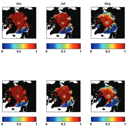
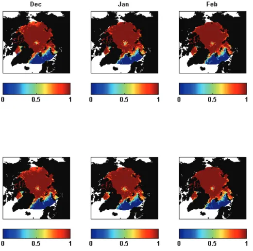
3.1 Inversion frequency

The composites of the mean inversion frequency (2003–2008) for the individual sum-mer and winter months are shown in Figs. 1 and 2, respectively. Di_fferences in the inversion frequency in the ascending and the descending passes are very small. This is in a way expected considering the stability of the atmosphere and small diurnal vari-20

(6)

ACPD

10, 2835–2858, 2010

Title Page

Tables Figures

◭ ◮

Back Close

Full Screen / Esc

Interactive Discussion When averaged over the entire study area (70◦_N–90◦_{N), the inversion frequency in}

summer ranges from 69% to 84% for the ascending passes and 72% to 86% for the descending passes. For winter, the frequency values are 88% to 91% for the ascending passes and 89% to 92% for the descending passes.

Such high values of inversion frequencies, even in summer, and their ubiquitous na-5

ture over the certain locations in the inner arctic in both summer and winter seasons have been previously reported. For example, Serreze et al. (1992) using rawinsonde data and Soviet Drifting Station data show that the parts of Eurasian Arctic Ocean experience inversion frequencies greater than 80% even in summer, while the frequen-cies are very close to 100% in winter (esp. over inner Arctic). More recently, Tjernstr ¨om 10

and Graversen (2009) using one year in-situ data (1997–1998) from the Surface Heat Budget of the Arctic (SHEBA) experiment, over the region located north of Alaska, re-ported that the inversions were practically present (99.5%) in all of their soundings. Our analysis results compare well with their findings.

3.2 Inversion strength

15

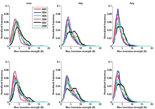
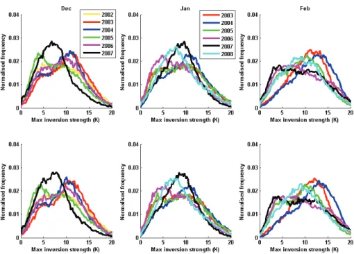
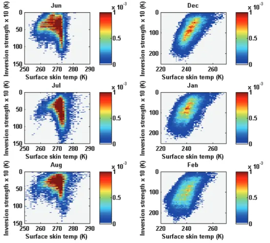
The PDFs of the inversion strength for the summer and winter months are shown in Figs. 3 and 4, respectively. The bin size on thex-axis is 0.25 K. The PDFs are plotted for all individual months and years separately and are computed for the entire study area. The PDFs in the summer months are narrow and right-skewed (or positively skewed). The inter-annual variability in the distribution is evident in the plots. The distri-20

butions for the years 2003, 2004, 2006, and 2008 follow approximately similar pattern, while the years 2005 and even more so 2007 stand out clearly showing much broader distributions. The year 2007 experienced one of the lowest sea-ice minimum events. The PDFs show that the inversions were very strong in summer of 2007 compared to “normal” years. The PDFs in 2007 also have the dual peak structure. The mean val-25

(7)

ACPD

10, 2835–2858, 2010

Title Page

Tables Figures

◭ ◮

Back Close

Full Screen / Esc

Interactive Discussion entire study area range from 7.8 K to 8.9 K (DJF 2002–2008). The standard deviation

of the inversion strength is about 1.5 K for the summer months, while it is about 3.0 K for winter months. Since the differences in the ascending and the descending passes are very small, only the analysis of the ascending passes is presented hereafter for brevity.

5

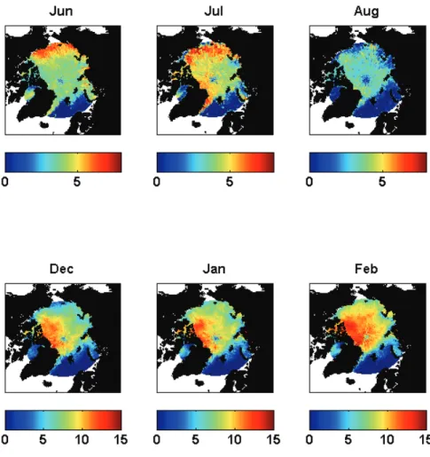
The spatial structure of the inversion strength from the ascending passes is shown in Fig. 5. Top row shows the mean composites for the summer months (2003–2008) and the bottom row for the winter months. Note that the scale of inversion strength is doubled for the winter months. East Siberian Sea and the Beaufort Sea show very high inversion strength in the range of 4 K to 8 K (in mean values) in June months. In 10

July, additionally the parts of western Greenland Sea and the Lincoln Sea also show high inversion strength. The inversion strength is reduced considerably in August. In December and January months, the area north of Greenland and the northeastern parts of North American Arctic show very high inversion strength ranging from 7 K to 15 K (in mean values). In February, the entire inner Arctic show very high inversion 15

strength. The intricate pattern of spatial variability in inversion strength is evident for all cases.

Previous studies also report a similar range of magnitudes of the inversion strength for winter. For example, Serreze et al. (1992) show that the mean inversion strength for the Eurasian Arctic ranges from 8 K to 12 K. Kahl et al. (1996) used nearly 30 000 20

temperature profiles over the Arctic Ocean (from 1950–1990) and showed the median inversion strength ranging from 6 K to 12 K. For the SHEBA experiment area, Tjern-str ¨om and Graversen (2009) computed the inversion Tjern-strength in the range of 8 K to 10 K. Liu et al. (2006), using HIRS sensor data, estimated the inversion strength in the range of 8 K to 15 K over the Arctic Ocean. The spatial pattern of the inversions 25

strength in their study closely matches with our results in winter.

(8)

sur-ACPD

10, 2835–2858, 2010

Title Page

Tables Figures

◭ ◮

Back Close

Full Screen / Esc

Interactive Discussion face temperature and inversion strength (for summer and winter months composited

for 2003–2008). The negative correlation between surface temperature and inversion strength can be seen for the winter months. Since the formation mechanisms of inver-sion are most likely to be different in summer and winter months (radiation loss being the main controlling factor in winter, while the advection of warm air from low latitudes 5

dominating in summer resulting in elevated inversions), it is also not expected that the similar relationship between the surface temperature and the inversion strength will hold true for summer. This is also clearly reflected in Fig. 6.

3.3 The summer of 2007

The record Arctic sea-ice minimum of summer 2007 has drawn a lot of attention (Deser 10

and Teng, 2008; Drobot et al., 2008; Giles et al., 2008; Kay et al., 2008; L’Heureux et al., 2008; Perovich et al., 2008; Schweiger et al., 2008; Vihma et al., 2008; Zhang et al., 2008; Kauker et al., 2009; Kay and Gettelman, 2009; Lindsay et al., 2009). The roles of clouds, radiation, circulation, atmospheric preconditioning and ice-albedo feedback etc, and their relevance in the context of long-term changes in the Arctic sea ice and the 15

2007 ice minimum event have been studied extensively over the past few years, using both modeling and observational approaches. Since changes in the inversion strength and its inter-annual variability are the manifestations of the interplay of these various atmospheric processes, the aim of this section is to provide some further crucial pieces of information in this context.

20

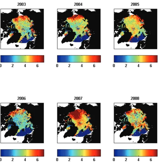
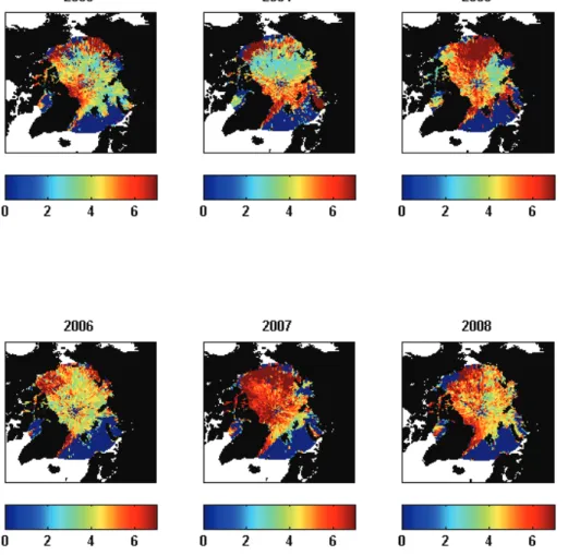
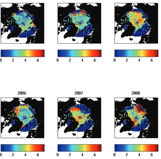
The spatial pattern of inversion strength and its inter-annual variability for June, July and August months are shown in Figs. 7, 8, and 9, respectively. In general, the East Siberian Sea and Beaufort Sea show high inversion strengths in June and July for all years (>5 K). However in 2007, the mean inversion strength over the Beaufort Sea shows a conspicuous enhancement (>6 K) in June, while in July, almost the entire Arc-25

(9)

av-ACPD

10, 2835–2858, 2010

Title Page

Tables Figures

◭ ◮

Back Close

Full Screen / Esc

Interactive Discussion erage of the remaining years (2003, 2004, 2005, 2006, and 2008). The lower and

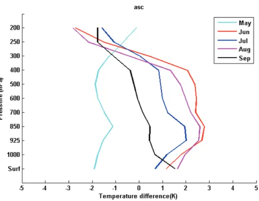
mid-troposphere was warmed by 1.5 K to 3.0 K in the summer months. Note that the warming was not restricted to the lowermost troposphere, and was observed up to 400 hPa level. Kay et al. (2008) have shown that the zonal and the vertical structure of the temperature over Arctic shows similar warming pattern in the summer months 5

of 2007 when compared to the previous year. Figure 10 shows that the month of June experienced the strongest warming in the lower troposphere which steadily decreased till September. Kay and Gettelman (2009) using radiosonde and AIRS data over the Barrow station also show similar feature for the summer of 2007.

3.4 Limitations of the present study

10

We use Level 3 data at the coarser spatial resolution of 1x1 deg rather than the Level 2 data in the present study. Considering the atmospheric stability of the region and the number of observations from the multiple passes of the satellite, the aggregation of L2 data into 1x1 degree grid box should not induce a signif-icant sampling bias. The number of L3 profiles used for the analysis is shown 15

in supplementary Fig. S1 (http://www.atmos-chem-phys-discuss.net/10/2835/2010/ acpd-10-2835-2010-supplement.pdf). We argue that the statistics presented here us-ing the vertical and spatial resolutions of the L3 data are su_fficient and relevant to allow direct comparison of our results with the statistics from most of the climate models.

We do not separate the surface-based and elevated inversions. Such categorization 20

is possible using the temperature profiles from the L2 Support Product provided at 100 vertical levels. However, this product is not rigorously validated yet. In future, it would be interesting to explore this issue further. One source of uncertainty could be the contamination of fractional clouds in the temperature profiles. However, the bias induced due to such situations is expected to be of very small magnitude (Susskind et 25

(10)

ACPD

10, 2835–2858, 2010

Title Page

Tables Figures

◭ ◮

Back Close

Full Screen / Esc

4 Conclusions and outlook

Since the changes in the inversion frequency and strength could provide direct hint of the climate change in Arctic and also influence the related processes, their accurate quantification and monitoring becomes crucial. The AIRS instrument provides a unique opportunity to quantify and monitor the inversion frequency and strength over the Arctic 5

Ocean at unprecedented accuracy and resolutions. For the first time, we quantify these parameters for the summer and winter months of 2003 to 2008 over the entire Arctic Ocean for clear-sky conditions. The results from our analysis are in general agreement with the previous studies that use radiosonde observations or the results from the special campaigns.

10

The following salient features emerged from our analysis:

1. Although the inversion frequency along the coastal regions in the Arctic decreases from June to August, inversions are still seen in almost every profile retrieved over the inner Arctic region.

2. In winter, inversions are ubiquitous over the inner Arctic and are present in the 15

every AIRS profile analysed.

3. When averaged over the entire study area (70◦_N–90◦_{N), the inversion frequency} in summer ranges from 69% to 86% for the ascending passes and 72% to 86% for the descending passes. For winter, the frequency values are 88% to 91% for the ascending passes and 89% to 92% for the descending passes.

20

4. The PDFs of inversion strength for the summer months are narrow and right-skewed (or positively right-skewed), while in winter, they are much broader.

5. In summer months, the mean values of inversion strength for the entire study area range from 2.5 K to 3.9 K, while in winter, they range from 7.8 K to 8.9 K. The standard deviation of the inversion strength is double in winter compared to 25

(11)

ACPD

10, 2835–2858, 2010

Title Page

Tables Figures

◭ ◮

Back Close

Full Screen / Esc

Interactive Discussion 6. Inversions in the summer months of 2007 were very strong compared to other

years. The warming in the troposphere of about 1.5 K to 3.0 K is observed ex-tending up to 400 hPa in the summer months of 2007.

It is of utmost importance that the global and regional climate models capture these inversion statistics and the vertical temperature structure as accurately as possible 5

to be able to realistically simulate and forecast the Arctic climate and the potential changes therein. The comparison of the statistics presented here with the Rossby Center regional models (Jones et al., 2004a, b) is currently undergoing. Few studies also indicate trends in inversion characteristics (Kahl et al., 1996; Liu et al., 2006). It is necessary to revisit such trends using integrated in-situ and satellite datasets to better 10

understand and to relate to the observed climate change in Arctic. The data from the Infrared Atmospheric Sounding Interferometer (IASI) instrument would provide even better vertical resolution so as to resolve different inversion types accurately.

Acknowledgement. The authors gratefully acknowledge the AIRS Science Team and GES DISC (NASA) for making the AIRS products freely available for research. This work was sup-15

ported by the Swedish National Space Board grant.

References

ACIA: Impacts of a warming Arctic: Arctic Climate Impact Assessment, Cambridge University Press, New York, 2004.

Bradley, R. S., Keimig, F. T., and Diaz, H. F.: Climatology of surface based inversions in the 20

North American Arctic, J. Geophys. Res., 94, 15699–15712, 1992.

Deser, C. and Teng, H.: Evolution of Arctic sea ice concentration trends and the role of atmospheric circulation forcing, 1979–2007, Geophys. Res. Lett., 35, L02504, doi:10.1029/2007GL032023, 2008.

Divakarla, M. G., Barnet, C. D., Goldberg, M. D., McMillin, L. M., Maddy, E., Wolf, W., Zhou, L., 25

(12)

ACPD

10, 2835–2858, 2010

Title Page Abstract Introduction Conclusions References Tables Figures ◭ ◮ ◭ ◮ Back Close

Full Screen / Esc

Interactive Discussion Drobot, S., Stroeve, J., Maslanik, J., Emery, W., Fowler, C., and Kay, J.: Evolution of the 2007–

2008 Arctic sea ice cover and prospects for a new record in 2008, Geophys. Res. Lett., 35, L19501, doi:10.1029/2008GL035316, 2008.

Fetzer, E. J.: Preface to special section: validation of atmospheric infrared sounder observa-tions, J. Geophys. Res., 111, D09S01, doi:10.1029/2005JD007020, 2006.

5

Gao, W., Zhao, F., and Gai, C.: Validation of AIRS retrieval temperature and moisture products and their application in numerical models, Acta Meteorol. Sin., 64, 271–280, 2006.

Giles, K. A., Laxon, S. W., and Ridout, A. L.: Circumpolar thinning of Arctic sea ice following the 2007 record ice extent minimum, Geophys. Res. Lett., 35, L22502, doi:10.1029/2008GL035710, 2008.

10

Jones, C. G., Will ´en, U., Ullerstig, A., and Hansson, U.: The Rossby centre regional atmo-spheric climate model part I: model climatology and performance for the present climate over Europe, Ambio, 33(4–5), 199–210, 2004a.

Jones, C. G., Wyser, K., Ullerstig, A. and Will ´en, U.: The Rossby centre regional atmospheric climate model part II: application to the Arctic Climate, Ambio, 33(4–5), 211–220, 2004b. 15

Kahl, J. D. W., Martinez, D. A., and Zaitseva, N. A.: Long-term variability in the low-level inver-sion layer over the Arctic Ocean, Int. J. Climatol., 16, 1297–1313, 1996.

Kahn, B. H. and Teixeira, J.: A global climatology of temperature and water vapour variance scaling from the Atmospheric Infrared Sounder, J. Climate, 22, 5558–5576, 2009.

Kauker, F., Kaminski, T., Karcher, M., Giering, R., Gerdes, R., and Voßbeck, M.: Adjoint 20

analysis of the 2007 all time Arctic sea-ice minimum, Geophys. Res. Lett., 36, L03707, doi:10.1029/2008GL036323, 2009.

Kay, J. E. and Gettelman, A.: Cloud influence on and response to seasonal Arctic sea ice loss, J. Geophys. Res., 114, D18204, doi:10.1029/2009JD011773, 2009.

Kay, J. E., L’Ecuyer, T., Gettelman, A., Stephens, G., and O’Dell, C.: The contribution of cloud 25

and radiation anomalies to the 2007 Arctic sea ice extent minimum, Geophys. Res. Lett., 35, L08503, doi:10.1029/2008GL033451, 2008.

L’Heureux, M. L., Kumar, A., Bell, G. D., Halpert, M. S., and Higgins, R. W.: Role of the Pacific-North American (PNA) pattern in the 2007 Arctic sea ice decline, Geophys. Res. Lett., 35, L20701, doi:10.1029/2008GL035205, 2008.

30

Lindsay, L. W., Zhang, J., Schweiger, A., Steele, M., and Stern, H.: Arctic Sea ice retreat in 2007 follows thinning trend, J. Climate, 22, 165–176, 2009.

(13)

ACPD

10, 2835–2858, 2010

Title Page Abstract Introduction Conclusions References Tables Figures ◭ ◮ ◭ ◮ Back Close

Full Screen / Esc

Interactive Discussion inversions with MODIS, J. Atmos. Ocean. Tech., 20, 1727–1737, 2003.

Liu, Y., Key, J. R., Schweiger, A., and Francis, J.: Characteristics of satellite-derived clear-sky atmospheric temperature inversion strength in the Arctic, 1980–96, J. Climate, 19, 4902– 4913, 2006.

Mernild, S. H. and Liston, G. E.: The influence of air temperature inversions on snowmelt 5

and glacier mass-balance simulations, Ammassalik Island, SE Greenland, J. Appl. Meteorol. Clim., in press, doi:10.1175/2009JAMC2065.1, 2009.

Olsen, E. T., Susskind, J., Blaisdell, J., and Rosenkranz, P.: AIRS/AMSU/HSB Version 5 Level 2 Quality Control and Error Estimation, Technical Report, JPL, NASA, USA, 15 pp., 2007a. Olsen, E. T., Granger, S., Manning, E., and Blaisdell, J.: AIRS/AMSU/HSB Version 5 Level 3 10

Quick Start, 25 pp., 2007b.

Perovich, D. K., Richter-Menge, J. A., Jones, K. F., and Light, B.: Sunlight, water, and ice: extreme Arctic sea ice melt during the summer of 2007, Geophys. Res. Lett., 35, L11501, doi:10.1029/2008GL034007, 2008.

Schweiger, A. J., Zhang, J., Lindsay, R. W., and Steele, M.: Did unusually sunny skies 15

help drive the record sea ice minimum of 2007?, Geophys. Res. Lett., 35, L10503, doi:10.1029/2008GL033463, 2008.

Sedlar, J. and Tjernstr ¨om, M.: Stratiform cloud-inversion characterization during the Arctic melt season, Bound.-Lay. Meteorol., 132, 455–474, doi:10.1007/s10546-009-9407-1, 2009. Serreze, M. C., Kahl, J. D., and Schnell, R. C.: Low-level temperature inversions of the Eurasian 20

Arctic and comparisons with Soviet drifting stations, J. Climate, 5, 615–630, 1992.

Susskind J., Barnet, C., Blaisdell, J., Iredell, L., Keita, F., Kouvaris, L., Molnar, G., Chahine, M.: Accuracy of geophysical parameters derived from atmospheric infrared sounder/advanced microwave sounding unit as a function of fractional cloud cover, J. Geophys. Res., 111, D09S17, doi:10.1029/2005JD006272, 2006.

25

Tjernstr ¨om, M. and Graversen, R. G.: The vertical structure of the lower Arctic troposphere analysed from observations and ERA-40 reanalysis, Q. J. Roy. Meteor. Soc., 135, 431–443, 2008.

Vihma, T., Jaagus, J., Jakobson, E., and Palo, T.: Meteorological conditions in the Arctic Ocean in spring and summer 2007 as recorded on the drifting ice station Tara, Geophys. Res. Lett., 30

(14)

ACPD

10, 2835–2858, 2010

Title Page

Tables Figures

◭ ◮

Back Close

Full Screen / Esc

Interactive Discussion Zhang, J., Lindsay, R., Steele, M., and Schweiger, A.: What drove the dramatic

(15)

ACPD

10, 2835–2858, 2010

Title Page

Tables Figures

◭ ◮

Back Close

Full Screen / Esc

Fig. 1. The mean inversion frequency (averaged over 2003–2008) for the summer months over

(16)

ACPD

10, 2835–2858, 2010

Title Page

Tables Figures

◭ ◮

Back Close

Full Screen / Esc

(17)

ACPD

10, 2835–2858, 2010

Title Page

Tables Figures

◭ ◮

Back Close

Full Screen / Esc

Fig. 3. The PDFs of inversion strength (in K) for the summer months. Top and bottom rows

(18)

ACPD

10, 2835–2858, 2010

Title Page

Tables Figures

◭ ◮

Back Close

Full Screen / Esc

(19)

ACPD

10, 2835–2858, 2010

Title Page

Tables Figures

◭ ◮

Back Close

Full Screen / Esc

Fig. 5. The spatial pattern of inversion strength (in K) averaged over 2003–2008 for summer

(20)

ACPD

10, 2835–2858, 2010

Title Page

Tables Figures

◭ ◮

Back Close

Full Screen / Esc

Fig. 6. The joint histograms of inversion strength and surface temperature for summer (left

(21)

ACPD

10, 2835–2858, 2010

Title Page

Tables Figures

◭ ◮

Back Close

Full Screen / Esc

Fig. 7. Inter-annual variations in the inversion strength (in K) for the month of June. Notice that

(22)

ACPD

10, 2835–2858, 2010

Title Page

Tables Figures

◭ ◮

Back Close

Full Screen / Esc

(23)

ACPD

10, 2835–2858, 2010

Title Page

Tables Figures

◭ ◮

Back Close

Full Screen / Esc

(24)

ACPD

10, 2835–2858, 2010

Title Page

Tables Figures

◭ ◮

Back Close

Full Screen / Esc

Fig. 10. The vertical structure of the monthly mean temperature anomalies during the summer