Uncertainties in isoprene photochemistry and emissions: implications for the oxidative capacity of past and present atmospheres and for trends in climate forcing agents

(1)

ACPD

15, 2197–2246, 2015

Uncertainties in isoprene photochemistry and

emissions

P. Achakulwisut et al.

Title Page

Abstract Introduction

Conclusions References

Tables Figures

◭ ◮

Back Close

Full Screen / Esc

Printer-friendly Version Interactive Discussion

Discussion

P

a

per

|

Discussion

P

a

per

|

Discussion

P

a

per

|

Discussion

P

a

per

|

Atmos. Chem. Phys. Discuss., 15, 2197–2246, 2015 www.atmos-chem-phys-discuss.net/15/2197/2015/ doi:10.5194/acpd-15-2197-2015

This discussion paper is/has been under review for the journal Atmospheric Chemistry and Physics (ACP). Please refer to the corresponding final paper in ACP if available.

Uncertainties in isoprene photochemistry

and emissions: implications for the

oxidative capacity of past and present

atmospheres and for trends in climate

forcing agents

P. Achakulwisut1, L. J. Mickley2, L. T. Murray3,4, A. P. K. Tai5, J. O. Kaplan6, and

B. Alexander7

1

Department of Earth and Planetary Sciences, Harvard University, Cambridge, MA, USA

2

School of Engineering and Applied Sciences, Harvard University, Cambridge, MA, USA

3

NASA Goddard Institute for Space Studies, New York, NY, USA

4

Lamont-Doherty Earth Observatory, Columbia University, Palisades, NY, USA

5

Earth System Science Programme, The Chinese University of Hong Kong, Hong Kong, China

6

ARVE Group, Ecole Polytechnique Fédérale de Lausanne, Lausanne, Switzerland

7

(2)

ACPD

15, 2197–2246, 2015

emissions

Title Page

Tables Figures

◭ ◮

Back Close

Full Screen / Esc

Discussion

P

a

per

|

Discussion

P

a

per

|

Discussion

P

a

per

|

Discussion

P

a

per

|

Received: 29 December 2014 – Accepted: 6 January 2015 – Published: 23 January 2015

Correspondence to: P. Achakulwisut (pachakulwisut@fas.harvard.edu)

(3)

ACPD

15, 2197–2246, 2015

emissions

Title Page

Tables Figures

◭ ◮

Back Close

Full Screen / Esc

Discussion

P

a

per

|

Discussion

P

a

per

|

Discussion

P

a

per

|

Discussion

P

a

per

|

Abstract

Current understanding of the factors controlling biogenic isoprene emissions and of the fate of isoprene oxidation products in the atmosphere has been evolving rapidly. We use a climate-biosphere-chemistry modeling framework to evaluate the sensitivity of estimates of the tropospheric oxidative capacity to uncertainties in isoprene

emis-5

sions and photochemistry. Our work focuses on trends across two time horizons: from the Last Glacial Maximum (LGM, 21 000 years BP) to the preindustrial (1770s); and from the preindustrial to the present day (1990s). We find that different oxidants have different sensitivities to the uncertainties tested in this study, with OH being the most sensitive: changes in the global mean OH levels for the LGM-to-preindustrial transition

10

range between−29 and+7 %, and those for the preindustrial-to-present day transition range between −8 and +17 %, across our simulations. Our results suggest that the observed glacial-interglacial variability in atmospheric methane concentrations is pre-dominantly driven by changes in methane sources as opposed to changes in OH, the primary methane sink. However, the magnitudes of change are subject to

uncertain-15

ties in the past isoprene global burdens, as are estimates of the change in the global burden of secondary organic aerosol (SOA) relative to the preindustrial. We show that the linear relationship between tropospheric mean OH and tropospheric mean ozone photolysis rates, water vapor, and total emissions of NO_xand reactive carbon – first re-ported in Murray et al. (2014) – does not hold across all periods with the new isoprene

20

(4)

ACPD

15, 2197–2246, 2015

emissions

Title Page

Tables Figures

◭ ◮

Back Close

Full Screen / Esc

Discussion

P

a

per

|

Discussion

P

a

per

|

Discussion

P

a

per

|

Discussion

P

a

per

|

1 Introduction

A key player in the coupling between climate change and atmospheric chemical com-position is the oxidative capacity of the troposphere, primarily characterized by the burden of the four most abundant and reactive oxidants: OH, ozone, H₂O₂, and NO₃. Estimates of the oxidative capacity of past atmospheres remain uncertain due to the

5

limited number of historical and paleo-observations, which hinders our ability to un-derstand the chemical, climatic, and ecological consequences of past changes in the oxidative capacity. Multiple factors govern the abundance of tropospheric oxidants, in-cluding emissions of reactive volatile organic compounds (VOCs). Isoprene (2-methyl-1,3-butadiene, C₅H₈), primarily emitted by plants, is the most abundant VOC in the

10

present-day atmosphere after methane (Pike and Young, 2009). Recent studies have suggested the need to revise our understanding of the environmental factors controlling biogenic isoprene emissions and of its atmospheric photo-oxidation mechanism (e.g., Paulot et al., 2009a, b; Possell and Hewitt, 2011). These advances call into question the validity of existing model estimates of the oxidative capacity of past atmospheres.

15

In this study, we use a climate-biosphere-chemistry modeling framework (Murray et al., 2014) to explore the sensitivity of the simulated oxidative capacity to uncertainties in isoprene emissions and photochemistry, and the implications for radiative forcing on preindustrial-present and on glacial-interglacial timescales. To our knowledge, this study is the first systematic evaluation of the effects of these recent developments on

20

model estimates of the chemical composition of past atmospheres.

The atmospheric oxidative capacity determines the lifetime of many trace gases im-portant to climate, chemistry, and human health (e.g., Isaksen and Dalsøren, 2011; Fiore et al., 2012). It may also induce oxidative stress or alter the deposition of oxidized nutrients to terrestrial and marine ecosystem (Sitch et al., 2007; Paulot et al., 2013).

25

(5)

ACPD

15, 2197–2246, 2015

emissions

Title Page

Tables Figures

◭ ◮

Back Close

Full Screen / Esc

Discussion

P

a

per

|

Discussion

P

a

per

|

Discussion

P

a

per

|

Discussion

P

a

per

|

impossible for the past. Late 19th-century surface ozone measurements exist but their accuracy has been debated (Pavelin et al., 1999). Atmospheric oxidants, except for H2O2, are not directly preserved in the ice-core record, but post-depositional processes

impede quantitative interpretation of the H₂O₂ record (Hutterli et al., 2002). As sum-marized in Murray et al. (2014), Table 1, prior modeling studies that investigated past

5

changes in the abundance of tropospheric oxidants disagree on the magnitude and even the sign of change. Such discrepancies call into question our ability to quantify the relative roles of sources and sinks in driving past variations in atmospheric methane concentration. Previous studies attributed these variations to changes in wetland emis-sions, the dominant natural source of methane to the atmosphere (e.g., Khalil and

Ras-10

mussen, 1987; Brook et al., 2000). However, more recent modeling studies suggested that potential variations in OH – the primary sink for methane – may be larger than previously thought, driven by changes in biogenic VOC emissions (e.g., Kaplan, 2002; Valdes, 2005; Harder et al., 2007).

Tropospheric oxidants are strongly coupled through atmospheric photochemical

re-15

actions, and their abundance responds to meteorological conditions, changes in sur-face and stratospheric boundary conditions, and changes in emissions of key chemical species such as reactive nitrogen oxides (NOx =NO+NO2) and VOCs. Present-day

natural emissions of VOCs, which far exceed those from anthropogenic sources on a global scale, are dominated by plant isoprene emissions, which have an estimated

20

global source ranging from approximately 500 to 750 Tg yr−1 (Lathière et al., 2005; Guenther et al., 2006). This large emission burden is accompanied by high reactiv-ity; isoprene has an atmospheric chemical lifetime on the order of minutes to hours (Pike and Young, 2009). Isoprene and its oxidation products react with OH, ozone, and the nitrate radical, and are thus major players in the oxidative chemistry of the

tropo-25

(6)

Un-ACPD

15, 2197–2246, 2015

emissions

Title Page

Tables Figures

◭ ◮

Back Close

Full Screen / Esc

Discussion

P

a

per

|

Discussion

P

a

per

|

Discussion

P

a

per

|

Discussion

P

a

per

|

certainties in the preindustrial-to-present day changes in biogenic SOA burdens lead to large uncertainties in the anthropogenic direct and indirect radiative forcing estimates (e.g., Scott et al., 2014; Unger, 2014). Results from the Atmospheric Chemistry and Climate Model Intercomparison Project (ACCMIP) demonstrate that uncertainties re-main in our understanding of the long-term trends in OH and methane lifetime, and

5

that these uncertainties primarily stem from a lack of adequate constraints on natu-ral precursor emissions and on the chemical mechanisms in the current generation of chemistry-climate models (Naik et al., 2013). Recent field and laboratory findings have called into question prior estimates of global burdens of isoprene for the past and future atmospheres, and have revealed new details of the isoprene photo-oxidation

mecha-10

nism. First, isoprene emission from plants is well known to be strongly dependent on plant species and, for a given species, on environmental factors including tempera-ture, light availability, and leaf age (Guenther et al., 2012). However, recent empirical studies have shown that isoprene emission by several plant taxa is also inversely cor-related with atmospheric CO2 levels, but this relationship is not yet well-constrained

15

(e.g., Wilkinson et al., 2009; Possell and Hewitt, 2011). The biochemical mechanism for this e_ffect remains unresolved, but evidence suggests that CO₂concentration plays a role in partitioning carbon-substrate availability between the chloroplast and cytosol of a plant cell, and in mobilizing stored carbon sources (Trowbridge et al., 2012). Such bio-mechanisms involving a CO₂-dependence of isoprene emissions may have evolved

20

in plants long ago.

Second, recent field studies in major isoprene-emitting regions, such as the Ama-zon forest (Lelieveld et al., 2008), South East Asia (Hewitt et al., 2010), and China (Hofzumahaus et al., 2009), reported large discrepancies between measured and mod-eled HOx (OH+HO2) concentrations, suggesting that VOC oxidation under low-NOx

25

(7)

ACPD

15, 2197–2246, 2015

emissions

Title Page

Tables Figures

◭ ◮

Back Close

Full Screen / Esc

Discussion

P

a

per

|

Discussion

P

a

per

|

Discussion

P

a

per

|

Discussion

P

a

per

|

HO_x under low-NO_x conditions (e.g., Paulot et al., 2009a, b). In general, greater OH-recycling enhances the efficiency of atmospheric oxidation, while greater NOx-recycling

enhances the efficiency of ozone production. However, the improved mechanism is still unable to fully reconcile measured and modeled OH concentrations (Mao et al., 2012). Moreover, global and regional modeling studies indicate that the heterogeneous HO2

5

uptake by aerosols presents a potentially important HOx sink. There remains,

how-ever, considerable uncertainty in the magnitude of this sink and its impact on tropo-spheric chemistry (Thornton et al., 2008) Mao et al. (2013a) proposed a new scheme in which HO2uptake by aerosols leads to H2O rather than H2O2 formation, via

cou-pling of Cu(I)/Cu(II) and Fe(II)/Fe(III) ions. Since H₂O₂can be readily photolyzed to

10

regenerate OH, this new mechanism provides a more e_fficient HO_xremoval pathway. In support of the ICE age Chemistry And Proxies (ICECAP) project, Murray et al. (2014) developed a new climate-biosphere-chemistry modeling framework for sim-ulating the chemical composition of the present and past tropospheres, focusing on preindustrial-to-present and glacial-interglacial transitions. The Last Glacial Maximum

15

(LGM,∼19–23 kyr) spans the coldest interval of the last glacial period (∼11.5–110 kyr)

and is relatively well recorded in ice-core and sediment records, making the LGM-to-preindustrial transition a convenient glacial-interglacial analogue. Disparities in existing model studies of past tropospheric oxidant levels are partly due to differences in the model components of the Earth system allowed to vary with climate, and the di_ffering

20

degrees of complexity in the representation of those components (Murray et al., 2014). The ICECAP project is the first 3-D model framework to consider the full suite of key fac-tors controlling the oxidative capacity of the troposphere at and since the LGM, includ-ing the effect of changes in the stratospheric column ozone on tropospheric photolysis rates. Murray et al. (2014) found that: (1) the oxidative capacities of the preindustrial

25

(8)

ACPD

15, 2197–2246, 2015

emissions

Title Page

Tables Figures

◭ ◮

Back Close

Full Screen / Esc

Discussion

P

a

per

|

Discussion

P

a

per

|

Discussion

P

a

per

|

Discussion

P

a

per

|

the oxidative capacity over LGM-present day timescales are tropospheric mean ozone photolysis rates, water vapor abundance, and total emissions of NOxand reactive

car-bon.

In light of recent developments in our understanding of the isoprene photo-oxidation mechanism and of the sensitivity of plant isoprene emissions to atmospheric CO2

lev-5

els, we build on the model study by Murray et al. (2014) to explore the sensitivity of the simulated tropospheric oxidative capacity at and since the LGM, and the ramifi-cations for our understanding of the factors controlling the oxidative capacity. We also discuss the implications for trends in short-lived climate forcers and for interpreting the ice-core methane record. To our knowledge, this is the first model study to consider,

10

in a systematic manner, the e_ffect of all of the above developments on the chemical composition of the troposphere over the last glacial-interglacial time interval and the industrial era.

2 Method: model framework, model developments, and project description

2.1 The ICECAP model framework

15

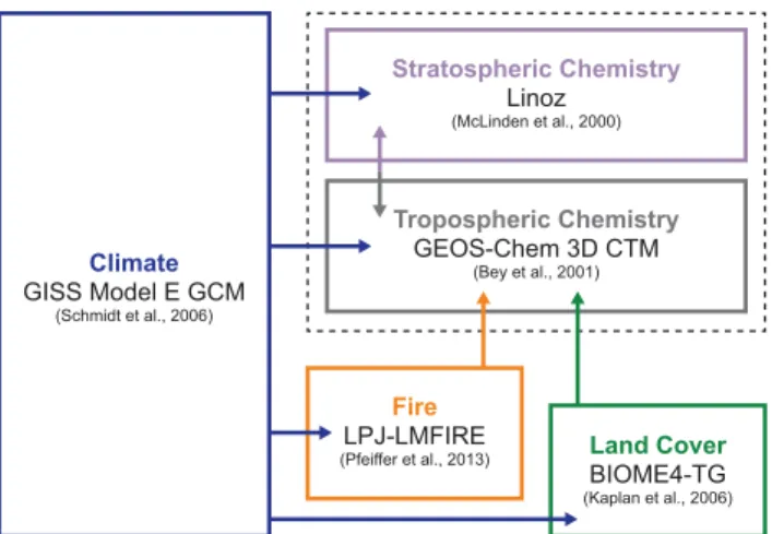
Figure 1 illustrates the stepwise, offline-coupled climate-biosphere-chemistry model framework of the ICECAP project. This setup relies on four global models. GEOS-Chem is a global 3-D chemical transport model (CTM) with a long history in sim-ulating present-day tropospheric ozone-NOx-CO-VOC-BrOx-aerosol chemistry (http:

//www.geos-chem.org; Bey et al., 2001; Park, 2004; Parrella et al., 2012), and includes

20

online linearized stratospheric chemistry (McLinden et al., 2000). We use version 9-01-03 with modifications as described in Murray et al. (2014) and below. ICECAP is driven by meteorological fields from ModelE, a climate model developed at the NASA Goddard Institute of Space Studies (GISS). ModelE and related models at GISS have been used extensively in paleo-climate studies (e.g., LeGrande et al., 2006; Rind et

25

(9)

ACPD

15, 2197–2246, 2015

emissions

Title Page

Tables Figures

◭ ◮

Back Close

Full Screen / Esc

Discussion

P

a

per

|

Discussion

P

a

per

|

Discussion

P

a

per

|

Discussion

P

a

per

|

latitude by 5◦longitude, and 23 vertical layers extending from the surface to 0.002 hPa in the atmosphere. Climate in ModelE is forced by prescribed greenhouse gas lev-els, orbital parameters, topography, and sea ice and sea surface temperatures (SSTs) relevant to each time slice of interest. The final components are the BIOME4-trace gas (BIOME4-TG) equilibrium terrestrial biosphere model (Kaplan et al., 2006) and

5

the Lund-Potsdam-Jena Lausanne-Mainz fire (LPJ-LMfire) dynamic global vegetation model (Pfei_ffer et al., 2013). BIOME4-TG is used to determine static vegetation distribu-tions, while LPJ-LMfire simulates biomass burning regimes. Meteorology from ModelE drives both these models, and the resulting land-cover characteristics and dry matter burned are implemented into GEOS-Chem. The o_ffline-coupling approach of ICECAP

10

allows sensitivity experiments to be performed relatively quickly. Also, by performing simulations in a stepwise manner, the chain of cause and effect can be readily diag-nosed. A detailed description of the ICECAP model framework and its evaluation can be found in Murray et al. (2014).

As in Murray et al. (2014), we perform simulations for four different climate scenarios:

15

present day (ca. 1990s); preindustrial (ca. 1770s); and two different representations of the LGM (∼19–23 kyr) to span the range of likely conditions. The two LGM scenarios differ in the degree of cooling of tropical SSTs. Such differences have implications for LGM dynamics because of the influence of tropical SSTs on meridional temperature gradients and low-latitude circulation (Rind et al., 2009). The “warm LGM” uses the

20

SST reconstructions from the Climate: long range Investigation, Mapping, and Predic-tion project (CLIMAP, 1976), with an average change in SST within 15◦of the equator relative to the preindustrial (∆SST15◦

S−◦_N) of−1.2 ◦

C. The “cold LGM” uses SSTs from Webb et al. (1997) who found ∆SST15◦_S

−◦_N of −6.1

◦

C by imposing an ocean heat transport flux in an earlier version of the GISS climate model. A more recent

esti-25

mate based on SST reconstructions from the MARGO project found∆SST15◦

S−◦_N of

(10)

ACPD

15, 2197–2246, 2015

emissions

Title Page

Tables Figures

◭ ◮

Back Close

Full Screen / Esc

Discussion

P

a

per

|

Discussion

P

a

per

|

Discussion

P

a

per

|

Discussion

P

a

per

|

Murray et al. (2014) also tested the sensitivity of their model results to uncertain-ties in lightning and fire emissions. Comparison with paleo-observations suggests that their “low-fire, variable-lightning, warm LGM” scenario was the best representation of the LGM atmosphere, in which lightning NO_x emissions are parameterized to reflect changes in convective cloud top heights, and the LPJ-LMfire fire emissions are scaled

5

to match observational records inferred from the Global Charcoal Database (Power et al., 2007, 2010). The model simulations in this study are performed using the Murray et al. (2014) “best estimate” fire and lightning emission scenarios relevant for each climate.

2.2 Uncertainties in biogenic isoprene emissions

10

Biogenic VOC emissions in GEOS-Chem are calculated interactively by the Model of Emissions of Gases and Aerosols from Nature (MEGAN v2.1) (Guenther et al., 2012). The canopy-level flux of isoprene is computed as a function of plant function type (PFT)-specific basal emission rate, scaled by activity factors (γ_i) to account for envi-ronmental controlling factors including temperature, light availability, leaf age, and leaf

15

area index (LAI). Tai et al. (2013) recently implemented an additional activity factor, γC, to account for the effect of atmospheric CO2 concentrations. They used the

em-pirical relationship from Possell and Hewitt (2011):γC=a/(1+abC), where the fitting

parametersaandbhave values of 8.9406 and 0.0024 ppm−1, respectively, andC rep-resents the atmospheric CO2 concentration (γC=1 atC=370 ppm). To date, Possell

20

and Hewitt (2011) studied the widest range of plant taxa and atmospheric CO₂ con-centrations. Their CO2-isoprene emission response curve shows a higher sensitivity

at sub-ambient CO2concentrations than others from similar studies (e.g., Wilkinson et

al., 2009), likely providing an upper limit of this effect for past climates.

Table 1 summarizes the prescribed CO2 mixing ratios and the estimated total

an-25

nual isoprene burdens with and without consideration of the CO2-sensitivity of plant

(11)

ACPD

15, 2197–2246, 2015

emissions

Title Page

Tables Figures

◭ ◮

Back Close

Full Screen / Esc

Discussion

P

a

per

|

Discussion

P

a

per

|

Discussion

P

a

per

|

Discussion

P

a

per

|

preindustrial, 78 % for the warm LGM, and 77 % for the cold LGM scenarios, relative to estimates that do not take into account the CO2-sensitivity.

Previous studies, which employ different global biogenic VOC emission models and land cover products to the ones used in this study, find that biogenic VOC emis-sions were 20–26 % higher in the preindustrial relative to the present day (Pacifico

5

et al., 2012; Unger, 2013). In this study, we estimate this value to be 8 % when the CO₂-sensitivity of plant isoprene emissions is not considered, and 25 % when the CO₂ -sensitivity is considered.

2.3 Uncertainties in the fate of the oxidation products of isoprene

2.3.1 Isoprene photo-oxidation mechanism

10

Murray et al. (2014) used the original GEOS-Chem isoprene photo-oxidation mecha-nism which is largely based on Horowitz et al. (1998). Here we apply recent updates to the mechanism by Mao et al. (2013c) and Paulot et al. (2009a, b). Daytime oxidation of isoprene by OH leads to the formation of hydroxyl-peroxy radicals (ISOPO2). The new

scheme includes a more explicit treatment of the production and subsequent reactions

15

of organic nitrates, acids, and epoxides from reactions of the ISOPO₂ radicals. Such reactions lead to greater HOx- and NOx-regeneration and recycling than in the original

mechanism, especially under low-NOx conditions, which is of particular relevance for

past atmospheres (Mao et al., 2013c). Beyond Mao et al. (2013c), we also change the stoichiometry of the (ISOPO2+HO2) reaction to that recommended by the laboratory

20

study of Liu et al. (2013), which has smaller uncertainties and leads to relatively smaller yields (by∼50 %) of HO_x, methyl vinyl ketone (MVK), and methacrolein (MACR) from

(12)

ACPD

15, 2197–2246, 2015

emissions

Title Page

Tables Figures

◭ ◮

Back Close

Full Screen / Esc

Discussion

P

a

per

|

Discussion

P

a

per

|

Discussion

P

a

per

|

Discussion

P

a

per

|

2.3.2 Heterogeneous HO2uptake by aerosols

As parameterized in the standard GEOS-Chem model, gaseous HO2uptake by

aque-ous aerosols leads to H2O2formation and has a γ(HO2) value typically less than 0.1,

whereγ(HO₂) is a measure of the e_fficacy of uptake, defined as the fraction of HO₂ collisions with aerosol surfaces resulting in reaction. (Note thatγ traditionally refers to

5

both the aerosol uptake efficiency and biogenic emissions flux activity factor.) Atmo-spheric observations, however, suggest that HO₂ uptake by aerosols may in fact not produce H2O2(de Reus et al., 2005; Mao et al., 2010). In light of these findings, Mao

et al. (2013a) implemented a new uptake scheme in GEOS-Chem, in which HO2

up-take yields H₂O via coupling of Cu(I)/Cu(II) and Fe(II)/Fe(III) ions, and we follow that

10

approach here. As in Mao et al. (2013a), we use the upper limit ofγ(HO2)=1.0 for all

aerosol types to evaluate the implications of this uptake for the HOx budgets and for

the fate of the oxidation products of isoprene.

2.4 Outline of model sensitivity experiments

Table 2 summarizes the different climate, chemistry and plant isoprene emission

sce-15

narios tested in this model study. For each climate scenario, we apply to GEOS-Chem the archived meteorology and land cover products from the “best estimate” fire and lightning emission scenarios from Murray et al. (2014). We test three different chem-istry schemes in GEOS-Chem: C1 uses the original isoprene chemchem-istry and original HO₂ uptake; C2 uses the new isoprene chemistry and original HO₂ uptake; and C3

20

uses the new isoprene chemistry and new HO2 uptake mechanisms. Each chemistry

scheme is tested either with (w) or without (wo) inclusion of the CO2-sensitivity of

bio-genic isoprene emissions, except for the present day. As Table 1 shows, consideration of the CO2-sensitivity for the present day results in only a 4 % change in the global

iso-prene burden (γC=1 at C=370 ppm), and so we assume that the present-day model

25

(13)

simula-ACPD

15, 2197–2246, 2015

emissions

Title Page

Tables Figures

◭ ◮

Back Close

Full Screen / Esc

Discussion

P

a

per

|

Discussion

P

a

per

|

Discussion

P

a

per

|

Discussion

P

a

per

|

tions match the isoprene emissions and photochemistry schemes used by Murray et al. (2014) in their “best estimate” scenarios. We perform 21 simulations in total.

Each GEOS-Chem simulation is initialized over 10 years, repeatedly using the first year of archived meteorology, to reach equilibrium with respect to stratosphere-troposphere exchange. We then perform 3 more years of simulations for analysis.

5

3 Results

3.1 Tropospheric mean oxidant burdens

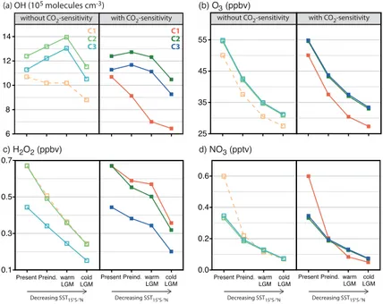
Figure 2 shows the simulated tropospheric mean mass-weighted burdens of OH, ozone, H2O2, and NO3 for each combination of climate, chemistry and plant isoprene

emission scenarios. The dotted orange line represents results using the “best

esti-10

mate” lightning and fire emission scenarios of Murray et al. (2014). The plots show the varying sensitivity of oxidant levels to assumptions about the tropospheric chemical mechanism and the global isoprene burden.

Consideration of the CO2-sensitivity of plant isoprene emissions yields larger

iso-prene emissions for the preindustrial and LGM scenarios (Table 1). For a given

chem-15

istry scheme and climate scenario, this leads to a decrease in the tropospheric mean OH burden, an increase in H2O2, and small changes in ozone and NO3. This result

can be understood by considering the classical tropospheric ozone-HOx-NOx-CO

cat-alytic cycle (e.g., Rohrer et al., 2014, Fig. 1). In general, daytime oxidation of VOC by reaction with OH leads to formation of oxidized organic products and HO₂. E_fficient

20

HOx-cycling depends on the presence of NOx. Since low-NOx conditions prevail in

past atmospheres, an increased isoprene burden represents a net OH sink but an HO2

source. The self-reaction of HO₂ leads to H₂O₂formation. Under low-NO_x conditions, tropospheric ozone production is relatively insensitive to changes in the reactive carbon burden. The tropospheric NO3burden also shows little change since the abundances

25

(14)

ACPD

15, 2197–2246, 2015

emissions

Title Page

Tables Figures

◭ ◮

Back Close

Full Screen / Esc

Discussion

P

a

per

|

Discussion

P

a

per

|

Discussion

P

a

per

|

Discussion

P

a

per

|

Implementation of the new isoprene oxidation mechanism leads to large changes in tropospheric oxidant burdens of OH, O3, and NO3, but not H2O2, for the present and

past atmospheres. Uncertainties in the isoprene mechanism are the largest source of uncertainties in global mean OH. Increases in the tropospheric mean OH burdens re-sult from greater HOx-regeneration in the new isoprene photo-oxidation cascade (Mao

5

et al., 2013c). The ozone production efficiency – the number of ozone molecules pro-duced per molecule of NO_x consumed (Liu et al., 1987) – is greater in the new iso-prene mechanism, leading to increases in the tropospheric ozone burdens. This is because the newly added reactions of recycling of isoprene nitrates, formed in the (ISOPO₂+NO) reaction pathway, can lead to NO_x-regeneration, thereby representing

10

a less permanent NO_x sink than nitric acid (Paulot et al., 2012). The present-day bur-den of NO3shows a large decrease in response to the new isoprene oxidation scheme,

while those of the past atmospheres show little change. The muted NO3response for

the past atmospheres is due to two competing e_ffects in the new scheme: (1) an in-creased aerosol reactive uptake coefficient of NO3 radicals (from 10

−4

to 0.1) leading

15

to greater NO3 depletion (Mao et al., 2013c); and (2) increased abundances in both

NO₃ precursors (NO₂₊O₃) enhancing its formation. The latter e_ffect is due to greater NOx-recycling and regeneration in the new scheme through isoprene nitrate recycling,

and hence greater ozone production efficiency and increased lifetime of NOx reservoir

species. For the present-day, the increased abundances of NO₃precursors are smaller

20

than those of the past atmospheres. Finally, implementation of the new scheme of HO2

uptake by aerosols leads to significant decreases in the tropospheric mean OH and H₂O₂ burdens in all simulations. This is due to both the higher e_fficacy of uptake than previously assumed and the formation of H2O, instead of H2O2, as a by-product of the

uptake, yielding a more efficient HOxremoval pathway.

25

Despite uncertainties in the isoprene emissions and photochemistry, we find reduced levels of ozone, H2O2, and NO3in each combination of chemistry and isoprene

(15)

ACPD

15, 2197–2246, 2015

emissions

Title Page

Tables Figures

◭ ◮

Back Close

Full Screen / Esc

Discussion

P

a

per

|

Discussion

P

a

per

|

Discussion

P

a

per

|

Discussion

P

a

per

|

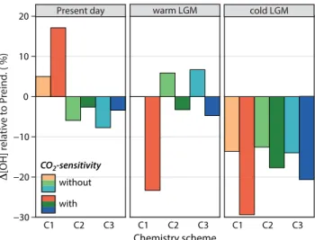
on glacial-interglacial timescales relative to other tropospheric oxidants does not hold for some of the uncertainties explored in this study. Figure 3 shows the simulated per-cent changes in the tropospheric mean OH burden for the present-day, warm LGM, and cold LGM scenarios, relative to their respective preindustrial scenarios. Consideration of the CO₂-sensitivity of plant isoprene emissions alone (C1-w) leads to 23 and 29 %

5

reductions in the tropospheric mean OH burden in the warm and cold LGM scenarios, relative to that of the preindustrial, while the present-day burden is 17 % greater than that of the preindustrial. When the new chemistry schemes are applied without consid-eration of the CO₂-sensitivity, the modeled changes in OH relative to the preindustrial are less dramatic but have opposite signs to those calculated under the C1-w scenarios

10

for the present day and warm LGM. When all effects are considered (C2-w and C3-w), changes in the tropospheric mean OH burden across the warm LGM-to-preindustrial and preindustrial-to-present day transitions do not exceed 5 %, a result consistent with Murray et al. (2014). The varying sensitivity of the tropospheric mean OH burden to as-sumptions about the isoprene photochemistry and emissions has implications for our

15

understanding of past methane and SOA burdens and radiative forcing calculations, as discussed in Sects. 3.3–3.4.

3.2 Comparison with observations

We evaluate the results of the model sensitivity experiments against four di_fferent cat-egories of observations. Table 3 compares the simulated methyl chloroform (CH3CCl3)

20

(16)

ACPD

15, 2197–2246, 2015

emissions

Title Page

Tables Figures

◭ ◮

Back Close

Full Screen / Esc

Discussion

P

a

per

|

Discussion

P

a

per

|

Discussion

P

a

per

|

Discussion

P

a

per

|

τX,OH=

TOA

R

surface

[X] dxdydz

tropopause

R

surface

kX+OH(T)[OH] [X] dxdydz

, (1)

where X represents either methyl chloroform or methane, and kX+OH(T) is the

temperature-dependent rate constant of the reaction. We assume that the mixing ratio of methyl chloroform is uniform throughout the troposphere and is 92 % lower than the total atmospheric concentration (Bey et al., 2001; Prather et al., 2012). For methane,

5

the global burden is calculated from the mean surface concentration – prescribed as 1743 ppbv for the present day – using a conversion factor of 2.75 Tg CH4ppbv

−1

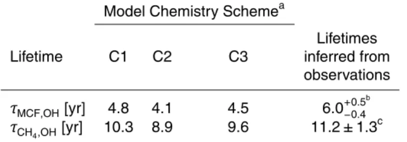
from Prather et al. (2012). The combination of new isoprene and original HO₂uptake chem-istry (C2) has the largest simulated tropospheric mean OH burden (Fig. 2) and so yields the shortest methyl chloroform and methane lifetimes: 4.1 and 8.9 years, respectively.

10

Prinn et al. (2005) inferred a methyl chloroform lifetime of 6.0+₋0.5_0.4years from observa-tions of methyl chloroform and knowledge of its emissions. Our model results are all lower than this range, but comparable to recent multi-model estimates of 5.7±0.9 years (Naik et al., 2013). Based on observations and emission estimates, Prinn et al. (2005) derived a mean methane lifetime of 10.2+−0.90.7 years between 1978–2004, and Prather

15

et al. (2012) derived a methane lifetime of 11.2±1.3 years for 2010. Although only the C1 value falls within this range, the slightly lower values given by the C2 and C3 chem-istry schemes are still within the range of estimates reported by recent multi-model studies: 10.2±1.7 years (Fiore et al., 2009), 9.8±1.6 years (Voulgarakis et al., 2013) and 9.7±1.5 years (Naik et al., 2013). Reconciling the magnitude of the inferred OH 20

(17)

ACPD

15, 2197–2246, 2015

emissions

Title Page

Tables Figures

◭ ◮

Back Close

Full Screen / Esc

Discussion

P

a

per

|

Discussion

P

a

per

|

Discussion

P

a

per

|

Discussion

P

a

per

|

0.98, whereas the recent ACCMIP multi-model study finds a mean ratio of 1.28±0.10

for 2000 (Naik et al., 2013; and references therein). For the years 2004–2011, Patra et al. (2014) finds an estimate of 0.97±0.12 by optimizing model results to fit methyl chloroform measurements. In our present-day sensitivity experiments, we find a ratio of 1.20 for C1, 1.11 for C2, and 1.07 for C3. The models participating in the ACCMIP

5

study did not consider HOx-recycling pathways through reactions of peroxy and HO2

radicals (Naik et al., 2013). As previously described, HO_x-recycling in the absence of NOx can occur in our new isoprene photochemistry scheme (C2), which leads to a

lower present-day N/S ratio of tropospheric mean OH. The decrease in this ratio is amplified when the upper limit of efficacy of HO₂uptake by aerosols is considered (C3),

10

because of large anthropogenic aerosol loadings in the Northern Hemisphere.

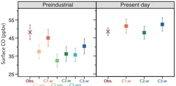
Figure 4 shows a comparison of CO surface concentrations over Antarctica between observations and our model results for the preindustrial and present-day simulations. CO influences the oxidative capacity of the troposphere through reaction with its pri-mary sink, OH, which can subsequently affect the ozone budget (Fiore et al., 2012). In

15

this context, CO can thus be a useful tool for evaluating the ability of chemistry transport models to simulate the tropospheric oxidative capacity (Haan and Raynaud, 1998). CO has a tropospheric lifetime of∼2 months (Novelli et al., 1998), and CO surface concen-trations over Antarctica are thus influenced by oxidation processes throughout much of the Southern Hemisphere (Haan and Raynaud, 1998; van der Werf et al., 2013)

20

. The NOAA Global Monitoring Division measured a mean CO surface concentration of 49±2 ppbv for the 1990s, which is matched by all of our present-day simulations tested with di_fferent chemistry schemes. Wang et al. (2010) recently provided a 650-year Antarctic ice-core record of concentration and isotopic ratios of atmospheric CO. They measured CO surface concentrations at the South Pole of 48±4 ppbv for the

25

year 1777 (±110 years). Only one (C1-w) out of the six preindustrial simulations tested

(18)

ACPD

15, 2197–2246, 2015

emissions

Title Page

Tables Figures

◭ ◮

Back Close

Full Screen / Esc

Discussion

P

a

per

|

Discussion

P

a

per

|

Discussion

P

a

per

|

Discussion

P

a

per

|

within the ice may complicate the comparison between ice-core CO and model results (Faïn et al., 2014; Guzmán et al., 2007; Haan and Raynaud, 1998).

Oxidants transfer unique isotopic signatures to the oxidation products, and we can take advantage of these signatures in our model evaluation if they are preserved in the ice-core record. The∆17O (=δ17O−0.52×δ18O) of sulfate, known as ∆17O(SO2₄−),

5

and of nitrate,∆17O(NO−₃), measure the departure from mass-dependent fractionation in its oxygen isotopes and reflect the relative importance of different oxidants in their atmospheric production pathways (Savarino et al., 2000). Sulfate formation primarily involves ozone, H2O2, and OH, while the main oxidants relevant to nitrate formation

are ozone, RO2 (R=H atom or organic group), OH, and BrO (Sofen et al., 2014).

10

Such oxygen triple-isotope measurements have been used to infer the atmospheric formation pathways of sulfate and nitrate in the present from atmospheric sulfate and nitrate (e.g. Lee et al., 2001; Michalski, 2003), and in the past from ice-core sulfate and nitrate (e.g., Alexander et al., 2002, 2004). The dominant source region for Antarctic sulfate is the Southern Ocean marine boundary layer (MBL) (Sofen et al., 2011), while

15

that for Antarctic nitrate is extra-tropical South America (Lee et al., 2014). We thus qualitatively compare our model results for these respective regions with Antarctic ice-core measurements of_∆17O(SO2₄−) and_∆17O(NO−₃).

Measurements of ∆17O(SO2₄−) from the WAIS Divide ice core imply that the [O3]/[OH] ratio in the Southern ocean MBL may have increased by 260 % since the

20

early 19th century, while measurements of_∆17O(NO−₃) suggest that the [O₃]/[RO₂] ratio in the Southern Hemisphere extratropical troposphere may have decreased by 60–90 % between the 1860s and 2000, assuming no change (≤5 %) in OH (Sofen et al., 2014). Table 4 lists the simulated percent changes in surface [O₃]/[OH] and [O3]/[RO2] in the present day scenarios relative to their respective preindustrial

scenar-25

ios. For [O3]/[OH], the signs of change are all consistent with the ice-core

(19)

abun-ACPD

15, 2197–2246, 2015

emissions

Title Page

Tables Figures

◭ ◮

Back Close

Full Screen / Esc

Discussion

P

a

per

|

Discussion

P

a

per

|

Discussion

P

a

per

|

Discussion

P

a

per

|

dance in the extra-tropical South American boundary layer in the present day would fur-ther lower∆17O(NO−₃), which is qualitatively consistent with the observations. However, accounting for both modeled decreases in [O3]/[RO2] and [OH] still underestimates

the observed decrease in∆17O(NO−₃) by 75–85 %. These mismatches may be due to deficiencies in our current understanding and model representation of remote marine

5

boundary layer sulfate formation and of nitrate formation, as suggested by Sofen et al. (2014). On glacial-interglacial timescales, measurements of∆17O(SO2₄−) from the Vostok ice core imply that gas-phase oxidation by OH contributed up to 40 % more to sulfate production during the last glacial period relative to the interglacial periods before and after (Alexander et al., 2002). Here our simulated percent changes in surface OH

10

concentrations over the Southern Ocean between the LGM and preindustrial scenarios are more comparable to the observations, with values ranging from 68 to 120 % for the warm LGM and 87 to 117 % for the cold LGM scenarios (Table 4). Ongoing measure-ments of the∆17O in ice-core sulfate and nitrate over the last glacial-interglacial cycle will allow for further model evaluation. Measurements of∆17O(NO−₃) may in fact be a

15

more robust proxy than those of ∆17O(SO2₄−) for reconstructing the oxidation capac-ity of past atmospheres because of its greater sensitivcapac-ity to oxidant abundances. For example, cloud amount and pH do not influence the isotopic composition of nitrate as they do for sulfate (Levine et al., 2011).

3.3 Implications for the methane budget

20

The global methane lifetime against oxidation by tropospheric OH,τCH₄,OH, is

calcu-lated as defined by Eq. (1). In GEOS-Chem, atmospheric methane concentrations are prescribed from observations – the tropospheric mean concentrations are 1743 ppbv for the present day, 731 ppbv for the preindustrial, and 377 ppbv for the LGM scenar-ios (Murray et al., 2014, Table 3). The approximately doubled methane concentration

25

(20)

ACPD

15, 2197–2246, 2015

emissions

Title Page

Tables Figures

◭ ◮

Back Close

Full Screen / Esc

Discussion

P

a

per

|

Discussion

P

a

per

|

Discussion

P

a

per

|

Discussion

P

a

per

|

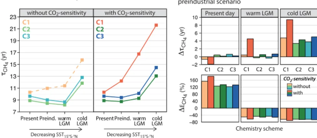
The left panels of Fig. 5 show the global methane lifetimes against oxidation by tropospheric OH for each combination of climate, chemistry, and isoprene emission scenarios. The dotted orange line represents results using the “best estimate” lightning and fire emission scenarios of Murray et al. (2014). Consideration of the CO₂-sensitivity of plant isoprene emissions alone leads to large increases in the past global isoprene

5

emissions, which in turn depress the tropospheric mean OH burden, thereby lengthen-ing the methane lifetimes by 1.2 years for the preindustrial, 5.4 years for the warm LGM, and 5.8 years for the cold LGM. Conversely, implementation of the new isoprene photo-oxidation scheme leads to larger OH burdens, resulting in decreases in the methane lifetimes – by 1.4 years for the present day, 2.6 years for the preindustrial, 3.2 years

10

for the warm LGM, and 4.0 years for the cold LGM. Implementation of the new HO₂ uptake scheme dampens the OH burden, which in turn slightly increases the methane lifetimes for each climate scenario.

We compare the sensitivity of the changes in the global methane lifetimes and in the implied emissions relative to the preindustrial in the right panels of Fig. 5.

Re-15

sults from the “best estimate” scenarios of Murray et al. (2014) suggest that relative to the preindustrial, the global methane lifetime is reduced by 0.7 years in the present, and is increased by 0.4 years at the LGM. This minimal increase in the lifetime at the LGM puts a higher burden on sources in explaining the glacial-interglacial vari-ability of atmospheric methane concentration. Assuming no large changes occurred

20

in the minor loss mechanisms, methane emissions scale with changes in its loss by OH in the troposphere. As defined in Sect. 3.2, the total loss rate of methane with respect to OH oxidation in the troposphere (Tg yr−1) is calculated from the integral:

tropopause

R

surface

kCH₄+OH(T)[OH] [CH4] dxdydz. For their “best estimate” scenarios, Murray et

al. (2014) reports that total methane emissions are 150 % higher in the present relative

25

to the preindustrial and are reduced by 50 % at the LGM. In our study, consideration of the CO2-sensitivity of plant isoprene emissions alone shortens the methane lifetime

(21)

ACPD

15, 2197–2246, 2015

emissions

Title Page

Tables Figures

◭ ◮

Back Close

Full Screen / Esc

Discussion

P

a

per

|

Discussion

P

a

per

|

Discussion

P

a

per

|

Discussion

P

a

per

|

at the LGM. This result suggests that methane emissions are reduced by 63 % at the LGM relative to the preindustrial, which places an even larger burden on sources than in Murray et al. (2014) in explaining the glacial-interglacial variability of atmospheric methane concentration. On the other hand, implementation of the new isoprene photo-oxidation scheme, either with or without consideration of the CO2-sensitivity of plant

5

isoprene emissions, results in relatively small changes in methane lifetimes across the glacial-interglacial or preindustrial-to-present day timescales. The resulting estimates of the reductions in methane emissions at the LGM relative to the preindustrial (be-tween 46–52 %) are consistent with the Murray et al. (2014) finding.

In summary, the calculated change in global methane lifetime at the LGM relative to

10

the preindustrial ranges between−0.4 to₊4.6 years across our ensemble of sensitivity

simulations. This range implies a reduction in methane emissions greater than or com-parable to the estimated value of 50 % by Murray et al. (2014) in their “best estimate” scenario. Our estimates are also greater than the 29–42 % decrease in wetland emis-sions simulated by the PMIP2 ensemble members (Weber et al., 2010), and the 16 and

15

23 % decreases in natural methane emissions simulated by Kaplan et al. (2006) and Valdes (2005), respectively.

3.4 Implications for SOA burdens and radiative forcing

Isoprene oxidation products substantially contribute to SOA formation (Henze and Se-infeld, 2006), and so our results have implications for trends in SOA burden and

ra-20

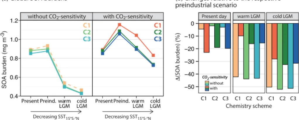
diative forcing. Increasingly cooler global temperatures relative to the present day in the preindustrial, warm LGM, and cold LGM scenarios are expected to decrease bio-genic isoprene emissions. However, such reductions are dampened or offset when the sensitivity to atmospheric CO₂ is also considered, since biogenic isoprene emissions are enhanced at CO2concentrations below present-day levels. The left panel of Fig. 6

25

(22)

ACPD

15, 2197–2246, 2015

emissions

Title Page

Tables Figures

◭ ◮

Back Close

Full Screen / Esc

Discussion

P

a

per

|

Discussion

P

a

per

|

Discussion

P

a

per

|

Discussion

P

a

per

|

of the CO₂-sensitivity of plant isoprene emissions alone leads to large increases in the past global isoprene burdens, which subsequently increases SOA at the preindustrial and LGM. For example, under the C1 chemistry scheme, the relative increases in the SOA burden are 24 % for the preindustrial, 93 % for the warm LGM, and 80 % for the cold LGM scenario when the CO2-sensitivity of plant isoprene emissions is considered

5

compared to the cases when it is not. Conversely, for a given isoprene emission sce-nario, changes to the isoprene photo-oxidation and HO₂uptake schemes lead to much smaller changes in the SOA burdens in each climate scenario.

The right panel of Fig. 6 shows the percent changes in tropospheric mean SOA bur-dens relative to their respective preindustrial scenarios. The “best estimate” scenarios

10

of Murray et al. (2014) – represented by our “C1-wo” simulations – suggest that relative to the preindustrial, the total SOA burden is 5 % lower in the present, 42 % lower at the warm LGM, and 50 % lower at the cold LGM. These values, while relatively robust to variations in the isoprene photo-oxidation and HO₂ uptake schemes, are sensitive to estimates of the global isoprene burdens for the past atmospheres; consideration of

15

the CO2-sensitivity of plant isoprene emissions enhances the present-to-preindustrial

di_fference but reduces the LGM-to-preindustrial di_fferences in the global SOA burden. For example, under the C1 chemistry scheme, consideration of the CO2-sensitivity of

plant isoprene emissions leads to decreases of 23 % in the total SOA burden in the present, but only of 10 and 28 % in the warm and cold LGM scenarios, relative to the

20

preindustrial.

3.5 Factors controlling variability in the tropospheric oxidative capacity

Murray et al. (2014) identified the key parameters that appear to control global mean OH levels on glacial-interglacial timescales. In this section, we explore the robustness of their result to the uncertainties in isoprene photochemistry and emissions tested in

25

this study. Using the steady-state equations of the ozone-NOx-HOx-CO system, Wang

(23)

ACPD

15, 2197–2246, 2015

emissions

Title Page

Tables Figures

◭ ◮

Back Close

Full Screen / Esc

Discussion

P

a

per

|

Discussion

P

a

per

|

Discussion

P

a

per

|

Discussion

P

a

per

|

the ratioSN/

S_C3/2, whereSNandSCare the tropospheric sources of reactive nitrogen

(Tmol N yr−1) and of reactive carbon (Tmol C yr−1), respectively. Murray et al. (2014) found that on glacial-interglacial timescales, the linear relationship can be maintained if two additional factors, which Wang and Jacob (1998) had assumed constant in their derivation, are also considered: (1) the mean tropospheric ozone photolysis frequency,

5

JO₃ (s

−1

) and (2) the tropospheric water vapor concentration, represented by the spe-cific humidity,q(g H2O kg air

−1

). In other words,

[OH]∝J_O 3q SN/

S_C3/2 (2)

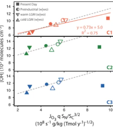
Figure 7 shows a plot of the tropospheric mean OH burden for each simulation as a function of JO₃q SN/

S_C3/2, divided into panels according to the chemistry scheme.

10

As in Murray et al. (2014), SC is calculated as the sum of emissions of CO and

NMVOCs and an implied source of methane equal to its loss rate by OH. While Murray et al. (2014) assumed that each molecule of isoprene yields an average 2.5 carbons that go on to react in the gas phase, this assumption has been found to not be robust for different isoprene oxidation schemes, and so we assume that each isoprene molecule

15

undergoes 100 % gas-phase oxidation for all of the three chemistry schemes tested in this study.

Only the C1 data subset shows a statistically significant correlation coefficient; a re-duced major axis regression fit is shown by the orange line (Fig. 7). The breakdown in linearity for the C2 and C3 subsets can by explained by examining the classical

tropo-20

spheric NOx-HOx-CO-ozone chemistry, upon which the linear relationship is derived.

In this classical chemistry system, HO_x-cycling is coupled to NO_x-cycling. However, the new isoprene photo-oxidation mechanism includes additional pathways for HOx

-regeneration and recycling in the absence of NOx. The new mechanism thus permits

HO_x-cycling to occur without subsequent production of ozone through NO₂

photoly-25

(24)

ACPD

15, 2197–2246, 2015

emissions

Title Page

Tables Figures

◭ ◮

Back Close

Full Screen / Esc

Discussion

P

a

per

|

Discussion

P

a

per

|

Discussion

P

a

per

|

Discussion

P

a

per

|

JO₃q SN/

S_C3/2. For example, Murray et al. (2014) found that the global mean OH independently varied weakly but most strongly with the photolysis component (JO₃) in

their simulations. In this study, the only subset of simulations exhibiting a statistically significant correlation between OH andJO₃ is C1-wo (R

2

=0.99, n=4). This scheme employs the original isoprene and HO2 uptake schemes without consideration of the

5

CO2-sensitivity of plant isoprene emissions – i.e., the same as that used by Murray et

al. (2014).

In Fig. 7, it can be seen that the slopes of the relationship appear to change be-tween the LGM-to-preindustrial and preindustrial-to-present day transitions for all of the three data subsets. We test whether the slope and intercept values are

signifi-10

cantly different between the chemistry schemes by fitting a multiple regression model withJO₃q SN/

S_C3/2 as a continuous explanatory variable and chemistry scheme as a categorical explanatory variable. We find that the three correlations have different values for the intercepts whereas the values for the slopes do not significantly differ (Fig. 7, dashed grey lines). The value of the intercept is largest for the C2 ensemble,

15

followed by C3, and then C1, indicating that mean OH is sensitive to the chemistry scheme used. This sequence follows from our finding that the new isoprene photo-oxidation mechanism leads to larger tropospheric mean OH burdens for each climate scenario compared to those simulated by the original mechanism. Implementation of the new HO2 uptake scheme dampens this increase, but values remain above those

20

from the C1 ensemble (Sect. 3.1). We postulate two main reasons why the slope of OH toJO₃q SN/

S_C3/2 appears to be lower across the industrial era than across the glacial-interglacial period. First, it is likely that heterogeneous reactions that can also act as HO_x sinks but are not considered in the derivation of the linear relationship, such as N2O5 hydrolysis and HO2 uptake by aerosols, become more important

un-25

(25)

tropo-ACPD

15, 2197–2246, 2015

emissions

Title Page

Tables Figures

◭ ◮

Back Close

Full Screen / Esc

Discussion

P

a

per

|

Discussion

P

a

per

|

Discussion

P

a

per

|

Discussion

P

a

per

|

spheric NO_x emissions. The ratio of lightning to surface NO_x emissions is 0.16 for the present day, 0.50 for the preindustrial, 0.73 for the warm LGM, and 0.79 for the cold LGM. The much lower present-day ratio is primarily due to large anthropogenic surface NO_x emissions, especially in the Northern Hemisphere (Murray et al., 2014, Fig. 5). This could lead to relatively more efficient NOx removal by wet and dry deposition,

5

and by formation of organic nitrates, which would both reduce primary and secondary OH production. However, these hypotheses need to be examined in greater detail, and an evaluation of potential weaknesses of the linear relationship between OH and JO₃q SN/

S_C3/2that operate independently of the classic photo-oxidation mechanism is described by Murray et al. (2015).

10

4 Discussion and conclusions

Using a detailed climate-biosphere-chemistry framework, we evaluate the sensitivity of modeled tropospheric oxidant levels to recent advances in our understanding of biogenic isoprene emissions and of the fate of isoprene oxidation products in the atmo-sphere. We focus on this sensitivity for the present day (ca. 1990s), preindustrial (ca.

15

1770s), and the Last Glacial Maximum (LGM,∼19–23 kyr). The 3-D global ICECAP model employed here considers the full suite of key factors controlling the oxidative capacity of the troposphere, including the effect of changes in the stratospheric column ozone on tropospheric photolysis rates (Murray et al., 2014). Our study, which revisits Murray et al. (2014), takes into account the sensitivity of plant isoprene emissions to

20

atmospheric CO2 levels, and considers the effects of a new isoprene photo-oxidation

(Paulot et al., 2009a, b) and a potentially larger role for heterogeneous HO2 uptake

Mao et al., 2013a). To our knowledge, this is the first model study to perform a sys-tematic evaluation of the sensitivity of the chemical composition of past atmospheres to these developments.

(26)

ACPD

15, 2197–2246, 2015

emissions

Title Page

Tables Figures

◭ ◮

Back Close

Full Screen / Esc

Discussion

P

a

per

|

Discussion

P

a

per

|

Discussion

P

a

per

|

Discussion

P

a

per

|

We simulate two possible realizations of the LGM, one significantly colder than the other, to bound the range of uncertainty in the extent of tropical cooling at the LGM. For each climate scenario, we test three different chemistry schemes: C1, the origi-nal isoprene chemistry and origiorigi-nal HO₂ uptake; C2, the new isoprene chemistry and original HO2uptake; and C3, the new isoprene chemistry and new HO2uptake

mecha-5

nisms. Each chemistry scheme is tested with or without inclusion of the CO2-sensitivity

of biogenic isoprene emissions, except for the present day for which consideration of the CO2-sensitivity results in only a 4 % change in the global isoprene burden. We

find that consideration of the CO2-sensitivity of biogenic emissions enhances plant

iso-prene emissions by 27 % in the preindustrial and by 77–78 % at the LGM, relative to

10

respective estimates that do not take into account the CO₂-sensitivity.

We find that different oxidants have varying sensitivity to the assumptions tested in this study, with OH being the most sensitive. Although Murray et al. (2014) estimated that OH is relatively well bu_ffered on glacial-interglacial timescales, we find that this result is not robust to all of the assumptions tested in this study, especially with respect

15

to uncertainties in the isoprene photo-oxidation mechanism. Changes in the global mean OH levels for the LGM-to-preindustrial transition range between−29 and ₊7 %,

and those for the preindustrial-to-present day transition range between−8 and+17 %, across our sensitivity simulations. However, consistent with Murray et al. (2014), we find reduced levels of ozone, H₂O₂, and NO₃for the past atmospheres relative to the

20

present-day in our ensemble of sensitivity simulations. That study also reported a linear relationship between OH and tropospheric mean ozone photolysis rates, water vapor, and total emissions of NOxand reactive carbon (JO₃q SN/

S_C3/2) on LGM-to-present day timescales. We find that the new isoprene photo-oxidation mechanism causes a breakdown in this linear relationship across the entire period, as the new mechanism

25

permits HO_x-cycling to occur without subsequent production of ozone through NO₂ photolysis, thereby weakening the feedback on OH production per RO2consumed. We

propose that the sensitivity of OH to changes inJO₃q SN/

(27)

ACPD

15, 2197–2246, 2015

emissions

Title Page

Tables Figures

◭ ◮

Back Close

Full Screen / Esc

Discussion

P

a

per

|

Discussion

P

a

per

|

Discussion

P

a

per

|

Discussion

P

a

per

|

preindustrial-to-present day than the LGM-to-preindustrial transition. This is most likely because NOx and HOx loss processes not considered in the classical NOx-HOx

-CO-ozone system (from which the linear relationship is derived) become more important under present-day conditions. All of our sensitivity experiments are broadly consistent with ice-core records of∆17O of sulfate and nitrate at the LGM and of CO in the

prein-5

dustrial. For the present-day, the C1 chemistry scheme shows the best agreement with observation-based estimates of methane and methyl chloroform lifetimes, whereas C3 shows the best agreement with observation-based estimates of the inter-hemispheric (N/S) ratio of tropospheric mean OH. Thus, it is challenging to identify the most likely chemistry and isoprene emission scenarios.

10

We find that the calculated change in global methane lifetime at the LGM relative to the preindustrial ranges between−0.4 to+4.6 years across our ensemble of sensitivity simulations. This range implies a reduction in methane emissions greater than or com-parable to the best estimate value of 50 % by Murray et al. (2014), which corroborates their finding that the observed glacial-interglacial variability in atmospheric methane is

15

predominantly driven by changes in its sources as opposed to its sink with OH. Our findings also have implications for radiative forcing estimates of SOA on preindustrial-present and glacial-interglacial timescales. For example, the “best estimate” scenarios of Murray et al. (2014) suggest that relative to the preindustrial, the total SOA burden is 5 % lower in the present and 42 % lower at the LGM. Here, we find decreases ranging

20

between 2–23 % in the present and 10–44 % at the LGM relative to the preindustrial across our sensitivity experiments. The climate effects of biogenic SOA are not well characterized, but are thought to provide regional cooling (Scott et al., 2014). Our work thus suggests that SOA reductions may have amplified regional warming in the present but minimized regional cooling at the LGM, relative to the preindustrial. Results from

25