Observing The Mediterranean Sea from space: 21 years of Pathfinder-AVHRR Sea Surface Temperatures (1985 to 2005). Re-analysis and validation

(1)

OSD

3, 1191–1223, 2006

21 years of Mediterranean SST.

Re-analysis and validation

S. Marull et al.

Title Page

Abstract Introduction

Conclusions References

Tables Figures

◭ ◮

Back Close

Full Screen / Esc

Printer-friendly Version

Interactive Discussion Ocean Sci. Discuss., 3, 1191–1223, 2006

www.ocean-sci-discuss.net/3/1191/2006/ © Author(s) 2006. This work is licensed under a Creative Commons License.

Ocean Science Discussions

Papers published inOcean Science Discussionsare under open-access review for the journalOcean Science

Observing The Mediterranean Sea from

space: 21 years of Pathfinder-AVHRR Sea

Surface Temperatures (1985 to 2005).

Re-analysis and validation

S. Marullo1, B. Buongiorno Nardelli2, M. Guarracino1, and R. Santoleri2

1

ENEA – Centro Ricerche Frascati, Via Enrico Fermi, 45, 00044 Frascati, Italia

2

CNR – Istituto di Scienze dell’Atmosfera e del Clima, Gruppo Oceanografia da Satellite, Via del Fosso del Cavaliere, 100, 00133 Roma, Italia

Received: 17 July 2006 – Accepted: 3 August 2006 – Published: 8 August 2006 Correspondence to: S. Marullo (salvatore.marullo@casaccia.enea.it)

(2)

OSD

3, 1191–1223, 2006

S. Marull et al.

Title Page

Tables Figures

◭ ◮

Back Close

Full Screen / Esc

Interactive Discussion

Abstract

The time series of satellite infrared AVHRR data from 1985 to 2005 has been used to produce a daily series of optimally interpolated SST maps over the regular grid of the operational MFSTEP OGCM model of the Mediterranean basin. A complete vali-dation of this OISST (Optimally Interpolated Sea Surface Temperature) product with in

5

situ measurements has been performed in order to exclude any possibility of spurious trends due to instrumental calibration errors/shifts or algorithms malfunctioning related to local geophysical factors. The validation showed that satellite OISST is able to re-produce in situ measurements with a mean bias of less than 0.1◦C and RMSE of about 0.5◦C and that errors do not drift with time or with the percent interpolation error.

10

1 Introduction

The atmospheric circulation over the Mediterranean area is dominated in winter by the westerlies regime and in summer by the tropical African circulation, that may give rise to subsidence phenomena influencing the Eastern Mediterranean basin. These cli-matic conditions determine large Sea Surface Temperature (SST) excursions between

15

summer and winter, and an important response to the large scale interannual variability of the atmospheric forcing over the area. On the other way round, the Mediterranean seasonal predictability appears to be closely linked to the SST variations, that may produce a feedback through modified heat exchange and transport, and through al-terations in the uptake of CO₂, with important implications on both numerical weather

20

prediction and climate research (e.g. Lionello et al., 2006).

In addition to the uncertainties related to the natural variability, it is still an open question how deeply the hydrological cycle of the region has been modified by the intense land usage and coastal urban development in recent years. Moreover, as a matter of fact, human activities in the coastal areas and marine resource exploitation,

25

such as open ocean oil extraction and industrial fisheries, are experiencing a constant

(3)

OSD

3, 1191–1223, 2006

S. Marull et al.

Title Page

Tables Figures

◭ ◮

Back Close

Full Screen / Esc

Interactive Discussion increase, significantly aff_{ecting the marine ecosystem.}

This large natural variability and the man-induced changes can not be managed without an advanced nowcasting/forecasting system. To this aim, the Mediterranean Forecasting System (MFS) program built up an operational system for the prediction of currents and biochemical elements in the Mediterranean basin and coastal/shelf

5

areas, developed through a Pilot Project (MFSPP) that lasted from 1999 to 2001, and an advanced project: Towards an Environmental Prediction (MFSTEP), that ended in early 2006. The overall scientific objectives of the program include the monitoring and modelling of the ecosystem fluctuations at the level of primary producers and for the time scales of weeks to months, but also a re-analysis of available measurements to

10

explore and better understand the mechanisms driving the Mediterranean dynamics and climate.

To this aim, the SST has been recognized as one of the key parameters: records of SST date back almost one century and satellite observations from infrared data cover now more than 20 years. As a consequence, high resolution/coverage SST data

15

obtained from satellite systems are now available not only for real-time assimilation in forecasting models, but also for interannual/decadal variability studies.

Within the last phase of MFSTEP, a complete re-analysis and interpolation on the MFSTEP OGCM (Ocean General Circulation Model) grid of AVHRR (Advanced Very High Resolution Radiometer) SST measurements from 1985 to 2005 has been

per-20

formed and is presented here. Interpolation of the SST field was required by the presence of data voids in infrared images, due to cloud cover, and to allow simpler assimilation in the numerical models.

As evidenced also by the Global Ocean Data Assimilation Experiment (GODAE) High-Resolution Sea Surface Temperature Pilot Project (http://www.ghrsst-pp.org/),

in-25

terpolation is far from being a fully solved problem, and it is still the object of several studies, while many diff_{erent solutions have already been proposed (e.g. Reynolds et} al., 2002; Kaplan et al. 1998; Santoleri et al., 1991). In fact, the algorithms applied may vary due to the diff_{erent characteristics of the area considered, to the di}ff_{erent sources}

(4)

OSD

3, 1191–1223, 2006

S. Marull et al.

Title Page

Tables Figures

◭ ◮

Back Close

Full Screen / Esc

Interactive Discussion of data and also to numerical limitations.

In this paper, the optimal interpolation scheme developed within MFSTEP is fully detailed. The interpolation scheme was significantly modified with respect to previous MFSPP one (Buongiorno Nardelli et al., 2002), and was used both for the near-real time production of SST maps and for the complete re-analysis of 1985–2005 AVHRR

5

data over the Mediterranean and Eastern Atlantic areas covered by MFSTEP OGCM model grid. The main scope of this work is thus to evaluate the impact of the interpola-tion algorithm used in the framework of MFSTEP on the accuracy of the SST field, and to assess the accuracy of the re-analyses in order to identify eventual biases that could discourage the application of these data for climate studies (e.g. to detect interannual

10

SST trends in the Mediterranean Sea), or to assimilate data in numerical models. The work clearly required also a further validation of the Pathfinder SST product over the Mediterranean Sea versus in situ data. Though AVHRR instruments sense the tem-perature of the surface skin layer (SST_skin), the validation has been performed with in situ bulk data instead of in situ SSTskin data (for a complete discussion on SST

defi-15

nitions see also Donlon et al., 2004). This was coherent with the assumption that our interpolated product (based only on night-time data) is representative of the so called foundation temperature (SSTfnd, i.e. the SST at the base of the diurnal mixing layer), and gave also the opportunity to go back to 1985 in the validation with a reasonable and nearly uniform amount of matchups. As a result, for the first time a validated time

20

series of 21 years of optimally interpolated daily SST fields at high resolution will be available for climatological studies.

The paper is organized as follows: the satellite and in situ data sets are described in Sect. 2. Section 3 is dedicated to the description of the optimal interpolation scheme used. The input data set and interpolated maps validation are presented in Sects. 4

25

and 5, respectively, while a brief summary and conclusions are discussed in Sect. 6.

(5)

OSD

3, 1191–1223, 2006

S. Marull et al.

Title Page

Tables Figures

◭ ◮

Back Close

Full Screen / Esc

2 Satellite and in situ data-set

2.1 Satellite SST

The SST data used in this paper are a Mediterranean subset of the AVHRR Pathfinder product version 5.0. Pathfinder is a joint NASA/NOAA project devoted to the produc-tion of global SST maps from 1985 to the present. Pathfinder data are available at

5

daily/4 km time/space resolution, for day and night passes separately, and are de-rived from 4-km Global Area Coverage (GAC) data (for more information regarding the version 5 of the Pathfinder data seehttp://www.nodc.noaa.gov/sog/pathfinder4km/

userguide.html). The Pathfinder algorithm is based on the NLSST (Non Linear Sea Surface Temperature) formulation developed by Walton (1988), Walton et al. (1990,

10

1998a, 1998b) with some modification introduced as a result of the analysis of the PFMDB (PathFinder Matchup Data Base). The NLSST algorithm has the following form:

SST_sat =_a+_bT₄+_c_(T₄₋_T₅₎_SST_guess+_d_(T₄₋_T₅_{) (sec}_ρ₋₁₎

where SSTsatis the satellite-derived SST estimate, T4 andT5are brightness

tempera-15

tures in AVHRR channels 4 and 5 respectively, SSTguessis a first-guess SST value, and ρis the satellite zenith angle. Coeffi_{cients a, b, c, and d are estimated from regression} analyses using co-located in situ and satellite measurements (hereafter “matchups”). To reduce the presence of spurious trends in the SST estimates, the PFSST coeffi -cients are estimated on a month by month basis at global scale. Matchups are

se-20

lected within a window of five months, centred on the month for which coeffi_{cients were} being estimated. This continuous update of the SST algorithm coeffi_{cients makes, in} principle, the Pathfinder algorithm suitable for studies of year to year SST variability and allows to estimate multi-year SST trends, once the meaning of the used SST has been fixed.

25

Considering that infrared spacecraft radiometers measure the brightness tempera-ture relative to the skin layer and that Pathfinder SSTs are derived using coeffi_cients

(6)

OSD

3, 1191–1223, 2006

S. Marull et al.

Title Page

Tables Figures

◭ ◮

Back Close

Full Screen / Esc

Interactive Discussion based on a regression with bulk temperatures, it follows that Pathfinder SST are

repre-sentative of the SSTskinfield minus a “mean value” of the SSTSkin–SSTbulktemperature diff_{erence. In other words, “the temperature di}ff_{erence between the bulk sensors and} the radiating skin is incorporated into the SST retrieval algorithms in an unresolved, statistical sense” (Minnet, 2003). This statement implies that Pathfinder SST estimates

5

taken in conditions that deviate from “mean” can significantly diff_{er from} correspond-ing in situ bulk measurements. This fact is confirmed by recent studies that compared satellite estimate to skin measurements rather than bulk measurements (e.g. Kearns et al., 2000). They found that, using skin measurements, the scatter of the diff_erences between in situ and satellite temperatures is about half of the corresponding estimate

10

made using bulk measurements (RMS about 0.33◦C instead of 0.5–0.7◦C). Further details on the processing and algorithms used for SST estimate can be found in the work of Kilpatrick et al. (2001) or inhttp://www.rsmas.miami.edu/groups/rrsl/pathfinder/

Algorithm/algo index.html.

For this particular work we selected only descending orbits in order to reduce the

15

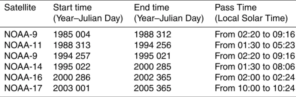
eff_{ect the diurnal cycle on the analysis of algorithms and interpolation performances.} Table I shows local solar time (LST) of the descending passes used for Pathfinder v5.

The Pathfinder SST product includes maps of flags that indicate whether each sin-gle SST estimate is contaminated by any environmental factor or not. The flags are obtained throughout a series of tests to assess the likelihood that a pixel

con-20

tains an SST value of suspect quality. The various tests are then combined to define eight overall quality levels for each pixel (see http://podaac.jpl.nasa.gov/pub/

sea surface temperature/avhrr/pathfinder/doc/usr gde4 0 toc.html for a detailed de-scription of flags). Of course the best SST estimates are those that have passed all the eight tests. We selected, as valid SST, those pixels that have passed all the tests

ex-25

cluding the reference test (the absolute diff_{erence between the Pathfinder SST for the} pixel considered and the reference Reynolds SST field must be less or equal to 2◦C). This last test has been ignored because another reference test is already included in our OA schema (see Sect. 3.2).

(7)

OSD

3, 1191–1223, 2006

S. Marull et al.

Title Page

Tables Figures

◭ ◮

Back Close

Full Screen / Esc

Interactive Discussion Valid Pathfinder data have been binned on MFSTEP OGCM grid at 1/16◦resolution

through a simple median of all valid measurements found within each grid cell. The median was preferred with respect to mean or weighted mean to further reduce the contamination by residual cloudy pixels eventually not flagged.

2.2 In situ data sets

5

The validation of the OISST time series has been performed with in situ data collected by diff_{erent sensors, and observational programs. The data used are described in the} following.

2.2.1 MEDAR/MEDATLAS XBT and CTD

MEDAR/MEDATLAS project made available a comprehensive data set of

oceano-10

graphic parameters collected in the Mediterranean and Black Sea, through a wide cooperation of the Mediterranean and Black Sea countries (Fischaut et al., 2002).

Actually, the MEDAR/MEDATLAS data base contains 36054 CTD casts and 161 890 XBT profiles from about 150 scientific laboratories of 33 countries. These data were submitted to automatic/objective and visual/subjective checks according to

interna-15

tional recommendations. As a result, a quality flag is assigned to each numerical value. The list of checks is detailed in the MEDATLAS protocol (http://www.ifremer.fr/medar).

We selected all the available XBT and CTD profiles covering the Mediterranean Basin from 1 January 1985 to 31 December 2004 excluding those XBT profiles al-ready included in the MFS data base. The MEDATLAS quality control flags were taken

20

into account to select only valid in situ measurements for the successive satellite data validation.

2.2.2 MFS XBT

Within the MFS-VOS (MFS-Voluntary Observing Ships) program, an extensive col-lection of temperature profiles by means of expendable Bathythermographs (XBTs)

25

(8)

OSD

3, 1191–1223, 2006

S. Marull et al.

Title Page

Tables Figures

◭ ◮

Back Close

Full Screen / Esc

Interactive Discussion was started since 1999 in the Mediterranean Sea. The XBT were launched from

ships of opportunities along selected tracks crossing the main Mediterranean sub-basins. The uncertainty on XBT temperature values was deeply evaluated by Re-seghetti et al. (2006a1, b2) versus simultaneous CTD measurements, and was found to be∼0.10◦C (i.e. comparable to the standard accuracy) in the surface layer. All

qual-5

ity controlled MFS-VOS data relative to the period 1999–2005 have been included in our matchup dataset (for a complete description of quality control procedures (see Re-seghetti et al., 2006b2).

2.2.3 MEDARGO floats

A large number of T/S profiles provided by autonomous profilers deployed in

10

the Mediterranean is currently available in the framework of the MFSTEP project through CORIOLIS data centre (http://www.coriolis.eu.org/cdc/projects/mfstep.htm). The MEDARGO-MFSTEP program has offi_{cially started its operational phase on 13} July 2004 and is still providing data today (Poulain et al., 20063). These floats oper-ate at a neutral parking depth of 350 m (near the salinity maximum of the Levantine

15

Intermediate Water) and are programmed to make periodic profiles of temperature and salinity from 700 m to surface. The floats reach the surface at intervals of 3–7 days. When at surface, the floats are located by and transmit data to the Argos system on-board the NOAA satellites. The data are processed and archived in near-real time at the CORIOLIS Data Center and are disseminated on the GTS following the standards

20

of the international ARGO program. Temperatures measured by ARGO profilers are

1

Reseghetti, F., Borghini, M., and Manzella, G. M. R.: Analysis of XBT data reliability in Western Mediterranean Sea, J. Atmos. Oceanic Technol., submitted, 2006a.

2

Reseghetti, F., Borghini M., and Manzella G. M. R.: Improved quality check procedures of XBT profiles in MFS-VOS. Ocean Sci., in preparation, 2006b.

3

Poulain, P.-M., Barbanti, R., Font, J., Cruzado, A., Millot, C., Gertman, I., Griff_{a, A., Rupolo,}

V., Le Bras S., and Petit de la Villeon, L.: MEDARGO: A Profiling Float Program in the Mediter-ranean Sea Ocean Sciences, Ocean Sci., in preparation, 2006.

(9)

OSD

3, 1191–1223, 2006

S. Marull et al.

Title Page

Tables Figures

◭ ◮

Back Close

Full Screen / Esc

Interactive Discussion accurate to±0.005◦C (http://www-argo.ucsd.edu/).

3 The optimal interpolation scheme

3.1 Background

The optimal interpolation (or statistical interpolation) method has been introduced many years ago to determine the optimal solution to the interpolation of a spatially

5

and temporally variable field with data voids, where “optimal” is intended in a least square sense (Gandin, 1965; Bretherton et al., 1976). Its basic principles are quickly reminded in the following. Consideringn observations Φ_obs _{given as the sum of the} “true” valueΦ_{plus a random error}_{ε, and assumed to have known mean}_<Φ_>_{and a} known and statistically stationary covariance,

10

Φ_obsi = Φ_i+ε_iε_iε_j=δ_{i j}ε2(i , j =1, . . ., n) (1)

hΦ_i=_known

the estimate ofΦ_{at a particular location}_x _{(in space and time), is obtained as a linear} combination of the observations:

ˆ Φ_(x)=

N X

i=1

α_i(x)Φ_obsi, (2)

15

where the coeffi_cients _α_i _{are obtained minimizing the error variance. The} Gauss-Markov theorem yields solution:

ˆ

Φ_(x)=_hΦ_i+ n X

i=₁ n X

j=₁

A−_{i j}1Cxj(Φobsi− hΦi), (3)

(10)

OSD

3, 1191–1223, 2006

S. Marull et al.

Title Page

Tables Figures

◭ ◮

Back Close

Full Screen / Esc

Interactive Discussion where the coeffi_cients_C_xj _and_A_{i j} _{are defined as:}

C_xi =_h₍Φ_(x)_{− h}Φ_i₎₍Φ_obs_i_{− h}Φ_i₎_i=_F_{(x, x}_i₎ ₍₄₎ A_{i j} =_h₍Φ_obsi − hΦi)(Φ_obsj − hΦi)i=C_{i j}+ε_iε_j

i.e. they represent the covariance of the field in the observations’ space and the to-tal covariance (signal covariance plus observation error covariance), respectively. In

5

general, A_{i j} elements (two-points correlations) are computed from a functional fit of the observation covariance values as a function of distance (in our case a “general-ized” space-time distance). This approach is called the Observational or Hollingworth-Lonnberg method. AlsoC_xi can be estimated in this way, taking the zero limit of the observed covariance function at zero distance and exactly the same values elsewhere.

10

The method also provides an estimate of the error variance, given by:

D

(Φ_(x)₋Φˆ_x₎2E=_C_xx₋ n X

i=1 n X

j=1

C_xiC_xjA−_{i j}1. (5)

All the above is rigorously valid only if it is possible to estimate the expected value of the field and to remove it from the observations. This is usually done computing an average of the data, and implies that there must be a suffi_{ciently large number of measurements.}

15

However, if the expected value cannot be computed as a simple average (example: not enough data), the theory discussed above still leads to a minimum error variance, provided that a suitable estimated mean is removed from the data. In that case, the coeffi_cients _C_xj _and _A_{i j}_{represent a structure function and di}ff_{er from the covariance} function by the unknown constant value<Φ_>2_:

20

Cxi =hΦ(x)Φobsii=R(x, xi)=F(x, xi)+hΦi 2

(6)

Ai j =hΦobsiΦobsji=Ci j+

εiεj ₊

hΦ_i2

(11)

OSD

3, 1191–1223, 2006

S. Marull et al.

Title Page Abstract Introduction Conclusions References Tables Figures ◭ ◮ ◭ ◮ Back Close

Full Screen / Esc

Interactive Discussion Independently of the value of this constant<Φ_>2_{, the new estimator is then given by:}

ˆ

Φ_(x)=Φ +˜ n X

i=1 n X

j=1

A−_{i j}1C_xj(Φ_obsi −Φ˜), (7)

where the estimated mean ˜Φ_{is computed from:} n

X

i=1 n X

j=1

A−_{i j}1(Φ_obsi −Φ˜)=0 (8)

i.e. weighting the observations with the observed structure function (Bretherton et al.,

5

1976). This procedure is generally called centering, and the new error estimate in-cludes an additional term:

D

(Φ_(x)₋Φˆ_x₎2E=_C_xx₋ n X

i=1 n X

j=1

CxiCxjA− 1 i j +

1−

n P i=1

n P j=1

C_xiA−_{i j}1 !2

n P i=₁

n P j=₁

Ai j

. (9)

As 3.9 depends on the structure function R, the interpolation error can be reduced introducing a first guess of the mean field Φ_g _{(constant) in the equations 3.6–3.9,}

10

provided that the new value of Cxx (computed with 3.10) is lower than this obtained through 3.6. The structure functions then become:

C_xi =

(Φ_(x)₋Φ_g₎₍Φ_obsi −Φ_g)=F(x, x_i)−2Φ_ghΦi+hΦi2=F(x, x_i)+H (10)

Ai j =

(Φ_obsi −Φ_g)(Φ_obsj −Φ_g)=C_{i j}+ε_iε_j+H

and the new estimator is:

15

ˆ

Φ_(x)= Φ_g+Φ +˜ n X

i=1 n X

j=1

A−_{i j}1C_xj(Φ_obsi −Φ_g−Φ˜) (11)

(12)

OSD

3, 1191–1223, 2006

S. Marull et al.

Title Page

Tables Figures

◭ ◮

Back Close

Full Screen / Esc

Interactive Discussion The estimated mean in that case would obviously be obtained assuming:

n X

i=1 n X

j=1

A−_{i j}1(Φ

obsi −Φg−Φ˜)=0, (12)

while the formula to estimate the error would remain the same as 3.9. This last ap-proach has been chosen in MFSTEP, taking as first guess a daily climatological decad field built from the dataset described in Sect. 2.1 but using only those SST values that

5

have passed all quality test (including also the reference test). In practice, each daily climatic map in this first guess field has been computed as the average over the whole 21 years period all the data within a 10 days moving window.

3.2 Description of the interpolation scheme

As the Mediterranean Sea is characterized by the presence of many islands and

penin-10

sulas, the scheme drives a “multi-basin” analysis to avoid data propagation across land from one sub-basin to the other. In practice, the optimal interpolation is run several times, one for each sub-basin, applying diff_{erent masks. Six sub-basin have been} iden-tified: Eastern Atlantic, Western Mediterranean basin, Tyrrhenian sea, Adriatic sea, Levantine basin, Aegean sea. In order to avoid artefact eff_{ects at the border of the}

15

diff_{erent regions, two di}ff_{erent masks are used for each sub-basin, one identifying the} interpolation points and one for the selection of the observations. This last includes buff_{er zones at the borders.}

The single analysis scheme includes diff_{erent modules and its details are described} in the following:

20

COVARIANCE/STRUCTURE MODEL: it is often unpractical, if not unfeasible in terms of computational time (as in the case of satellite SST data), to use all the data in a series to interpolate the field at a particular time, especially if the dominant scales of variability are shorter than the length of the time series. This is why most of the schemes first compute the covariance/structure function from all available data and

25

(13)

OSD

3, 1191–1223, 2006

S. Marull et al.

Title Page

Tables Figures

◭ ◮

Back Close

Full Screen / Esc

Interactive Discussion fit it to an analytical function (implicitly assuming statistical stationarity over the whole

time series), and successively introduce an influential radius, which represents the maximum (generalized) distance from the interpolation point over which observations are considered useful to the interpolation. In practice, the weights in expression 3.11 are computed directly from the analytical function, and only for a limited number of

ob-5

servations, reducing significantly the dimensions of the matrix to be inverted, as huge amounts of data in time and space are present in satellite datasets. Here, following the results by Marullo et al. (1998) and our recent researches within the Medspiration project (http://www.medspiration.org) on the main scales of SST variability, a separated dependence of the structure function from time and space lag has been adopted, and

10

the functional form was taken as:

C(r,∆_t)=_e−∆τt_e−Lr (13)

where r is the relative distance,∆_t_{is the time lag,}_L=_{180 km is a sort of spatial} “decor-relation” length andτ=_{7 days is a “temporal” decorrelation scale.}

IMAGES SELECTION: the first step in the processing chain includes in the analysis

15

only the images found within a temporal window (temporal influential radius) of –10/+₁₀ days with respect to the interpolation day (J) .

RESIDUAL CLOUDY PIXELS FLAGGING: successively, three tests are performed on all selected images prior to enter the interpolation, in order to avoid contamination by unflagged cloudy pixels. Firstly, cloud margins are eroded, flagging all values within

20

a distance ofmpixels to a pixel already flagged as cloudy. The second step consists in rejecting the SST values lower than a minimum threshold SST value (that can be changed seasonally). The third step is the comparison to the closer (in time) analysis available, that is used as a reference only if the analysis error (as defined in Sect. 3.1) is lower than a fixed value. Data that diff_{er from the reference field for more than a defined}

25

threshold (usually 2σ, where σ represents the average standard deviation between consecutive night images, estimated as 0.7◦C) are not included in the analysis. These “residual cloudy pixels flagging” tests contributed to flag residual clouds and many

(14)

OSD

3, 1191–1223, 2006

S. Marull et al.

Title Page

Tables Figures

◭ ◮

Back Close

Full Screen / Esc

Interactive Discussion other partially contaminated pixels avoiding the use of the Pathfinder reference test

that often fails in the Mediterranean Sea in areas where important hot or cold dynamical structures are present. A typical example is the Iera-Petra Gyre in the Levantine basin that most of the time is flagged by the Pathfinder reference test.

FIRST GUESS REMOVAL: coherently to the theory we have described in Sect. 3.1,

5

the following step consists in the removal from each input image of the corresponding decad climatological field.

INFLUENTIAL DATA SELECTION: as already pointed out, for each grid point obser-vations need to be selected within a space-time influential radius. However, only asub-set of these observations can eff_{ectively be used, because of computational time}

limi-10

tations. In Sect. 3.1, we have seen that the optimal interpolation behaves as a weighted mean of the observations, where the weights are directly related to the correlation be-tween the interpolation point and the single observations, but are reduced if the obser-vations are too much cross-correlated or have low accuracy. Consequently, a strategy to reduce the number of observations in input is to remove most cross-correlated data

15

following some a priori considerations. This strategy also reduces numerical problems raising from the inversion of nearly singular covariance matrices (singularity results from too much cross-correlation). Within MFSTEP, diff_{erent methodologies have been} tried, but very similar results have always been found. The method chosen is a bal-anced selection around the interpolation point in terms of spatial-temporal coverage,

20

that could be implemented due to the regularity of the grid on which data are orga-nized. The first step thus consists in sorting the data within the influential radius as a function of their correlation to the interpolation point. Successively, the most correlated observation is selected (i.e. included in the analysis), while all successive data are se-lected only if they are found along a new direction in space-time (until 50 observations

25

are found). This allows a more balanced coverage within the influential bubble, even selecting a small number of observations.

INTERPOLATION: the final step is performed estimating the terms Cxj and Ai j through the Function (3.13), and the mean of the selected observations through the

(15)

OSD

3, 1191–1223, 2006

S. Marull et al.

Title Page

Tables Figures

◭ ◮

Back Close

Full Screen / Esc

Interactive Discussion centering (3.12). Applying the expression (3.11), the optimal estimate is obtained.

This scheme has been applied to the whole data set from 1985 to 2005. An example of the OISST daily output and the climatological mean of all years are presented in Fig. 1a and b respectively.

4 Evaluation of Pathfinder product in the Mediterranean Sea

5

In order to evaluate the regional performances of the Pathfinder algorithm in the Mediterranean Sea respect to global ocean performances (Kearns et al., 2000; Min-net, 2003), we produced time series of co-located in situ and satellite measurements. Taking into account that in situ observation originate from a variety of sensors with dif-ferent errors, sensitivity and levels of quality control, we first performed the validation

10

separately for each dataset and sensor. More in detail the satellite and in situ match-up dataset was built for MEDATLAS/MEDAR and MFS-VOS XBT, MEDATLAS/MEDAR CTD and MEDARGO floats.

The space co-location criterion used to build the Mediterranean matchup files was set to less than 3.5 km between the measurement point and the centre of the

15

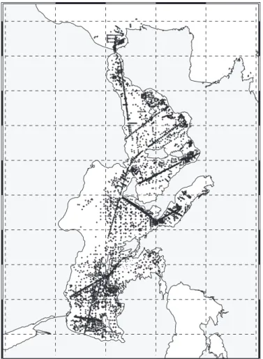
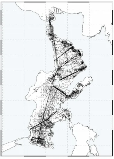
1/16◦×1/16◦pixel (i.e. the measurement point must fall within the binned satellite pixel). Figure 2 shows the spatial distribution of the selected matchup points. The time co-location criterion used was simply less than 12 h between satellite and in situ measure-ment.

To be consistent with previous definitions of SST_bulk (Donlon and the GRHSST

sci-20

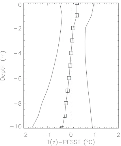
ence team, 2004) and to limit the eff_{ect of the diurnal cycle, for each temperature profile} the measurement closer to 3 m depth (in the range 2 m to 6 m depth) was selected. This choice was also supported by the analysis of the diff_{erence between temperature T at a} given depth z and corresponding PFSST (Fig. 3). The profile has been obtained using all the available matchup data points and averaging the diff_{erences at each depth. The}

25

absolute value of the mean bias was less than 0.1◦C between 2 and 6 m of depth. The minimum absolute diff_{erence between PFSST and T(z) was found at a depth of 4 m,}

(16)

OSD

3, 1191–1223, 2006

S. Marull et al.

Title Page

Tables Figures

◭ ◮

Back Close

Full Screen / Esc

Interactive Discussion where the bias is nearly zero with a standard deviation of 0.6◦C. The minimum RMSE

(∼0.5◦C) was found at 3 m, with a mean bias error close to zero.

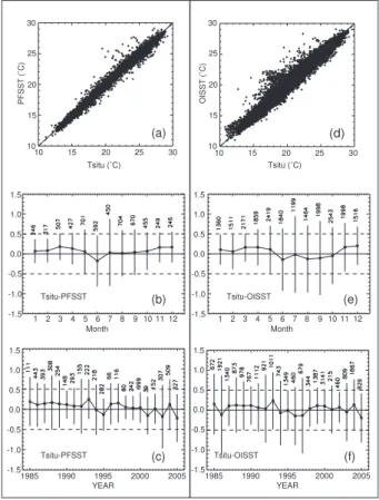
Table II summarizes the main statistical parameters characterizing the diff_erence between in situ and satellite measurement for each in situ dataset, and Fig. 4 shows the scatter plots for the three sources of data. The mean depth of the selected temperature

5

was 3.6 m.

The mean bias error (MBE=_{mean in situ – mean satellite) is quite satisfactory and} nearly stable for all instruments ranging from –0.16◦C to 0.10◦C. The higher diff_erences are found in the comparison with MEDARGO, with a negative MBE of –0.16◦C, due to the lack of MEDARGO measurements at depth lower than 4 m (mean reference depth

10

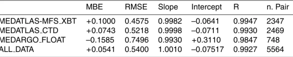
4.7 m) and coherently with what found in Fig. 3. The RMSE (standard deviation around the regression line) is very close to 0.5◦C for CTD and XBT, while it reaches 0.75◦C for MEDARGO. The regression line for XBTs and CTDs basically almost corresponds to the 1 to 1 perfect agreement line. MEDARGO regression line still has a slope very close to 1 but the intersect is 0.3◦C.

15

Averaging all data, the MBE is thus positive but small (+_0.05◦_{C) due to the relative} little amount of MEDARGO data with respect to the sum of XBT and CTD measure-ments (about 16% of the total). The RMSE values are anyway very close to previous estimates obtained from global data (e.g. Strong and McClain, 1984).

If MEDARGO data are not included in the analysis, the MBE reaches 0.08◦C, a value

20

very close to previous global estimates. In fact, diff_{erences between PFSST and in situ} SST_skin at night are expected to be 0.1±0.33◦C for mid- and low-latitudes (Kearns et al., 2000, Minnet, 2003) .

Figures 3 and 6 by Minnett (2003) show that the mean diff_{erence between SST}_skin and SST_3m varies depending on the true wind speed intensity, but this diff_{erence is,}

25

in general, around –0.2◦C at night, in most of the cases independently from the wind intensity.

(For night passes) PFSST – SST_Skin∼0.1◦C (after Kearns et al., 2000) (For Night measures) SSTSkin – SST3m∼–0.2

◦

C (after Minnet, 2003)

(17)

OSD

3, 1191–1223, 2006

S. Marull et al.

Title Page

Tables Figures

◭ ◮

Back Close

Full Screen / Esc

Interactive Discussion It follows that, on average at mid- and low-latitudes, the diff_{erence between SST}_3m

and PFSST should be about 0.1◦C, which is not so far from the results found. This is also in agreement with previous estimates of Pathfinder performances in the Mediter-ranean Sea made using an old version of Pathfinder algorithm for the years 1985–1994 (D’Ortenzio et al., 2000).

5

In the following, considering the uniform behaviour of the available source of data (see Table 2), we will continue our analysis using all the data as a single dataset.

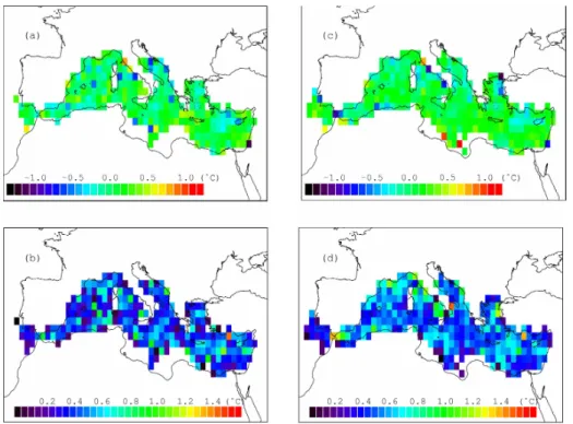
The spatial distribution of the in situ and satellite temperature diff_{erence (Fig. 5a)} and its standard deviation (Fig. 5b) is quite uniform and generally positive with few hot spots greater then 0.5◦C mostly located near the coasts.

10

First of all we evaluate the monthly behaviour of the diff_{erence between in situ and} satellite estimate in order to verify whether a seasonal signal was present or not. Figure 6b shows the mean monthly values of the bias between in situ measurements and satellite estimates. The MBE ranges from –0.17◦C in June to +_0.17◦_{C in December} with standard deviations comprised between 0.30◦C in February and 0.84◦C in July.

15

The tendency of the MBE to zero or to a slightly negative values during the warmer months (May, June, July, August and September) indicates the presence of a very small seasonal signal.

The behaviour of the yearly MBE permits to evaluate satellite eventual sensor drifts or shifts that could prevent the use of Pathfinder SST data to evaluate trends in the

20

SST of the Mediterranean Sea for the period 1985–2005. Figure 6c shows that the MBE does not significantly decrease/increase with years exhibiting a slope of – 0.01±0.02◦C/year (the standard deviations of each mean diff_{erence have been used to} estimate the uncertainty for the slope).

5 Validation of two decades of OISST

25

OISST maps were validate against in situ data using the same procedure applied in Sect. 4 for PFSST. The process produced a total of more than 21 000 matchups which

(18)

OSD

3, 1191–1223, 2006

S. Marull et al.

Title Page

Tables Figures

◭ ◮

Back Close

Full Screen / Esc

Interactive Discussion spatial distribution is shown in Fig. 7. Table 3 shows the main statistical parameters

that describe the diff_{erences between in situ measurements and Optimally Interpolated} SST (OISST). These statistical parameters are very similar to those of Tinsitu-PFSST (Table 2). The mean diff_{erence between XBT measurements and OISST estimates} re-mains more o less the same moving from 0.10◦C to 0.14◦C. For CTD the MBE becomes

5

slightly better than the previous value of 0.07◦C. In the case of MEDARGO floats the MBE is now closer to zero reaching the value of –0.06◦C.

Also the RMSE does not significantly change, even if a slight increase from 0.52◦C to 0.73◦C is observed in the case of CTD data and decrease from 0.75◦C to 0.69◦C is observed for MEDARGO floats resulting in an overall RMSE of 0.66◦C. Slopes and

10

intercepts as well as correlation coeffi_{cients remain basically unchanged. The scatter} plot of in situ measurement against OISST is shown in Fig. 6d.

The behaviour of the SSTinsitu-OISST on monthly and yearly basis is shown in Figs. 6e and f respectively. A first comparison with the corresponding figures obtained using PFSST (Figs. 6b and 6c) instead of OISST indicates that the OISST have not

15

introduced significant diff_{erences and that the main characteristics of the behaviour} re-mained unchanged. The use the MBE does not significantly decrease/increase with years, exhibiting a slope of 0.00±0.02◦C/year (the standard deviation of each mean diff_{erence have been used to estimate uncertainty for the slope).}

The MBE ranges from –0.14◦C in June to+_0.20◦_{C in December with standard}

devia-20

tions comprised between 0.36◦C in March and 0.96◦C in July. The tendency of the MBE to slightly negative values during the warmer months (June, July, August and October) indicates the presence of a very small seasonal signal similar to that already contained in the PFSST MBE time series.

Another interesting feature of the OISST estimates is the behaviour of the MBE and

25

RMSE as a function of the interpolation error. Figure 8 indicates that the MBE is es-sentially constant and very close to zero for interpolation errors less or equal 50%. For interpolation errors greater than this value, but less than 85% SSTinsitu-OISST ranges in the interval –0.19◦C to 0.08◦C. For interpolation errors greater or equal 90% the MBE

(19)

OSD

3, 1191–1223, 2006

S. Marull et al.

Title Page

Tables Figures

◭ ◮

Back Close

Full Screen / Esc

Interactive Discussion reaches values as high as 0.5◦C but, in this case the number of matchup points is very

small (only 12 matchups for 90% error and 11 for 95% error).

Concerning the spatial distribution of the SSTinsitu and OISST difference (Fig. 5c) and its standard deviation (Fig. 5d) only minor diff_{erences with respect to the patterns} seen for PFSST are found, with a slightly higher RMSE along the western coasts of the

5

Italian peninsula (Tyrrhenian and Ligurian Sea) and South coasts of France.

6 Summary and conclusion

Among the priorities of the Global Ocean Data Assimilation Experiment, it was clearly indicated the necessity to have an accurate and systematic estimate of the SST at high spatial resolution and daily repetitivity, mainly based on satellite measurements, with

10

no data voids, at global and regional scales. These requirements were driven both by climatological researches and by operational applications, with the final objective of monitoring, understanding and managing the natural variability and the man-induced changes to the marine ecosystem.

Within the MFSTEP program, an optimally interpolated SST product covering the

15

Mediterranean and Eastern Atlantic area at 1/16◦ resolution has been developed and produced in near-real-time for direct assimilation in MFSTEP large scale model. The hypothesis and assumptions behind MFSTEP optimal interpolation scheme have been fully described in this paper, detailing the characteristics of each module (from cloud detection to data selection, etc.) and justifying authors’ choices in the light of theoretical

20

and practical considerations.

The algorithm presented was then used to perform a re-analysis of Pathfinder SST time series, dating back to 1985. In fact, the main scope of the work was to evaluate the impact of MFSTEP interpolation scheme on the accuracy of the SST field, and to vali-date the 1985–2005 OISST time series. Comparing OISST and original Pathfinder SST

25

data (that were used as input data for the OI) with simultaneous MEDAR/MEDATLAS, MFS-VOS and MEDARGO measurements, it was possible to estimate the OISST

(20)

OSD

3, 1191–1223, 2006

S. Marull et al.

Title Page

Tables Figures

◭ ◮

Back Close

Full Screen / Esc

Interactive Discussion curacy in terms of mean bias error and standard deviation with respect to the SST

nearest to 3 m of depth (in the layer 2 m–6 m, see Sect. 4), assumed here as the best approximation to the foundation temperature. The results indicated that the impact of the OI is quite limited, with an increase in the RMSE from 0.54◦C to 0.66◦C and even a slightly better MBE (around 0.04◦C). Moreover, the sensitivity of both PFSST and

5

OISST accuracy to seasonal factors has been evaluated to be lower than 0.3◦C and, even more importantly, the presence of significant sensor drifts, shifts or responses to anomalous atmospheric events could be excluded by the present analysis. As a con-sequence, the MFSTEP OISST produced by the re-analysis of the PFSST represent a valuable dataset to investigate interannual and decade-to-decade variability of the SST

10

field, to detect trends and anomalously warm/cold years (e.g. 2003) and to investigate the role of local and remote forcing, also through assimilation in numerical models.

Acknowledgements. This study was funded by Mediterranean Forecasting Towards

Environ-mental Predictions (MFSTEP) and by Marine and EnviRonment and Security for European Area (MERSEA) European integrated projects. The AVHRR Oceans Pathfinder SST data were

15

obtained from the Physical Oceanography Distributed Active Archive Center (PO.DAAC) at the NASA Jet Propulsion Laboratory, Pasadena, CA,http://podaac.jpl.nasa.gov.

References

Bretherton, F. P., Davis, R. E., and Fandry, C. B.: A technique for objective analysis and design of oceanographic experiments applied to MODE-73. Deep Sea Res., 23, 559–582, 1976.

20

Buongiorno Nardelli, B., Larnicol, G., D’Acunzo, E., Santoleri, R., Marullo, S., and Le Traon, P. Y.: Near Real Time SLA and SST products during 2-years of MFS pilot project: processing, analysis of the variability and of the coupled patterns, Ann. Geophys., 20, 1–19. 2002. Donlon, C. J., Minnett, P. J., Gentemann, C., Nightingale, T. J., Barton, I. J., Ward, B., and

Mur-ray, J.: Towards improved validation of satellite sea surface skin temperature measurements

25

for climate research, J. Climate, 15, 353–369, 2002.

GHRSST-PP Science Team and ISDU-TAG working group: The Recommended GHRSST-PP Data Processing Specification GDS (Version 1 revision 1.5). GHRSST-PP Report Number

(21)

OSD

3, 1191–1223, 2006

S. Marull et al.

Title Page

Tables Figures

◭ ◮

Back Close

Full Screen / Esc

17. Published by the International GHRSST-PP Project Office; UK Met Office, United King-dom, 235 pp, 2004.

D’Ortenzio, F., Marullo, S., and Santoleri, R.: Validation of AVHRR Pathfinder SST’s over the Mediterranean Sea, Geophys. Res. Lett., 27, No. 2, 241–244, 2000.

Fichaut, M., Garcia, M.-J., Giorgetti, A., Iona, A., Kuznetsov, A., Rixen, M., and Group, M.:

5

MEDAR/MEDATLAS 2002: A Mediterranean and Black Sea database for the operational Oceanography, in Building the European Capacity in Operational Oceanography: Proceed-ings 3rd EuroGOOS Conference, Elsevier Oceanogr. Ser., 69, 645–648, 2002.

Gandin, L. S.: Objective analysis of meteorological ®elds. Israel Program for Scienti®c Trans-lation, Jerusalem, 242pp, 1965.

10

Kilpatrick, K. A., Podesta, G. P., and Evans, R.: Overview of the NOAA/NASA Advanced Very High Resolution Radiometer Pathfinder algorithm for sea surface temperature and associ-ated matchup database, J. Geophys. Res.-Oceans, 106(C5), 9179–9197, 15 MAY 2001. Kaplan, A., Cane, M. A., Kushnir, Y., Clement, A. C., Blumenthal, M. B., and Rajagopalan, B.:

Analyses of global sea surface temperature 1856–1991, J. Geophys. Res., 103(C9), 18 567–

15

18 590, doi:10.1029/98JC01736, 1998.

Kearns, E. J., Hanafin, J. A., Evans, R. H., Minnett, P. J., and Brown, O. B.: An indepen-dent assessment of Pathfinder AVHRR sea surface temperature accuracy using the Marine-Atmosphere Emitted Radiance Interferometer (M-AERI), Bull. Am. Meteorol. Soc., 81, 1525– 1536, 2000.

20

Lionello, P., Malanotte-Rizzoli, P., and Boscolo R.: The Mediterranean climate: an overview of the main characteristics and issues, Elsevier, Amsterdam, Netherlands, 2006.

Minnett, P. J.: Radiometric measurements of the sea-surface skin temperature: the competing roles of the diurnal thermocline and the cool skin, Int. J. Remote Sensing, 20 December 2003, 24(24), 5033–5047, 2003.

25

Reynolds, R. W., Rayner, N. A., Smith, T. M., Stokes, D. C., and Wang, W.: An improved in situ and satellite SST analysis for climate, J. Climate, 15, 1609–1625, 2002.

Santoleri, R., Marullo, S., and Bohm, E.: An Objective Analysis Schema for AVHRR Imagery, Int. J. Remote Sensing, 12, 681–693, 1991.

Strong, A. E. and McClain, E. P.: Improved ocean surface temperatures from space –

compar-30

isons with drifting floats, Bull. Am. Meteorol. Soc., 65, 138–142, 1984.

Walton, C. C., Pichel, W. G., Sapper, J. F., and May, D. A.: The development and 5046 P. J. Minnett operational application of nonlinear algorithms for the measurement of sea surface

(22)

OSD

3, 1191–1223, 2006

S. Marull et al.

Title Page

Tables Figures

◭ ◮

Back Close

Full Screen / Esc

temperatures with the NOAA polar-orbiting environmental satellites, J. Geophys. Res., 103, 27 999–28 012, 1998.

Walton, C. C., McClain, E. P., and Sapper, J. F.: Recent changes in satellite based multichannel sea surface temperature algorithms. Marine Technology Society Meeting, MTS’ 90, Wash-ington D.C, September 1990.

5

Walton, C. C., Pichel, W. G., Sapper, J. F., and May D.: The development and operational application of nonlinear algorithms for the measurement of sea surface temperatures with the NOAA polar-orbiting environmental satellites, J. Geophys. Res., 103(C12), 27 999–28 012, 1998a.

Walton, C. C., Sullivan, J. T., Rao, C. R. N., and Weinreb, M.: Corrections for detector

nonlin-10

earities and calibration inconsistencies of the infrared channels of the advanced very high resolution radiometer, J. Geophys. Res., 103(C2), 3323–3337, 1998b.

(23)

OSD

3, 1191–1223, 2006

S. Marull et al.

Title Page

Tables Figures

◭ ◮

Back Close

Full Screen / Esc

Interactive Discussion Table 1. Available satellite platforms during the period 1985–2005 and corresponding

acquisi-tion time.

Satellite Start time End time Pass Time

(Year–Julian Day) (Year–Julian Day) (Local Solar Time) NOAA-9 1985 004 1988 312 From 02:20 to 09:16 NOAA-11 1988 313 1994 256 From 01:30 to 05:23 NOAA-9 1994 257 1995 021 From 02:20 to 09:16 NOAA-14 1995 022 2000 285 From 01:30 to 08:06 NOAA-16 2000 286 2002 365 From 02:00 to 02:24 NOAA-17 2003 001 2005 365 From 10:00 to 10:24

(24)

OSD

3, 1191–1223, 2006

S. Marull et al.

Title Page

Tables Figures

◭ ◮

Back Close

Full Screen / Esc

Interactive Discussion Table 2. Statistical parameters characterizing the differences between in situ SST and

Pathfinder data.

MBE RMSE Slope Intercept R n. Pair MEDATLAS-MFS XBT +0.1000 0.4575 0.9982 –0.0641 0.9947 2347 MEDATLAS CTD +0.0743 0.5218 0.9998 –0.0711 0.9930 2469 MEDARGO FLOAT –0.1585 0.7496 0.9930 +0.3110 0.9847 748 ALL DATA +0.0541 0.5400 1.0010 –0.07517 0.9927 5564

(25)

OSD

3, 1191–1223, 2006

S. Marull et al.

Title Page

Tables Figures

◭ ◮

Back Close

Full Screen / Esc

Interactive Discussion Table 3.Statistical parameters characterizing the differences between in situ SST and OISST

data.

MBE RMSE Slope Intercept R n. Pair MEDATLAS MFS XBT 0.1365 0.5375 0.9966 –0.0709 0.9911 8521 MEDATLAS CTD 0.0002 0.7348 0.9868 0.2511 0.9826 11162 MEDARGO FLOAT –0.0620 0.6886 1.0026 0.0092 0.9870 2196 ALL DATA 0.04703 0.6645 0.9926 0.0963 0.9864 21879

(26)

OSD

3, 1191–1223, 2006

S. Marull et al.

Title Page

Tables Figures

◭ ◮

Back Close

Full Screen / Esc

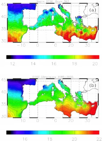
Interactive Discussion Fig. 1. An example of OISST daily map on 29 December 2000(a)and climatological mean of

all years(b).

(27)

OSD

3, 1191–1223, 2006

S. Marull et al.

Title Page

Tables Figures

◭ ◮

Back Close

Full Screen / Esc

Interactive Discussion Fig. 2.Spatial distribution of the selected PFSST matchup points.

(28)

OSD

3, 1191–1223, 2006

S. Marull et al.

Title Page

Tables Figures

◭ ◮

Back Close

Full Screen / Esc

Interactive Discussion Fig. 3. Vertical profile of the difference between PFSST and in situ temperature as function of

the depth z.

(29)

OSD

3, 1191–1223, 2006

S. Marull et al.

Title Page

Tables Figures

◭ ◮

Back Close

Full Screen / Esc

10 15 20 25 30

10 15 20 25

PFSST

XBT (˚C)

(a)

10 15 20 25 10 15 20 25 30

CTD (˚C) MEDARGO (˚C)

(b) (c)

Fig. 4. Scatter plots of PFSST against XBT measurements(a), CTD Measurements(b)and MEDARGO measuremenst(c).

(30)

OSD

3, 1191–1223, 2006

S. Marull et al.

Title Page

Tables Figures

◭ ◮

Back Close

Full Screen / Esc

Interactive Discussion Fig. 5.Spatial distribution of: Tsitu-PFSST(a)and its standard deviation(b); Tsitu-OISST(c)

and its standard deviation(d).

(31)

OSD

3, 1191–1223, 2006

S. Marull et al.

Title Page Abstract Introduction Conclusions References Tables Figures ◭ ◮ ◭ ◮ Back Close

Full Screen / Esc

10 15 20 25 30 10 15 20 25 30 OISST (˚C) Tsitu (˚C)

10 15 20 25 30 10 15 20 25 30 PFSST (˚C) Tsitu (˚C)

2 3 4 6

1 5 7 8 9 10 11 12 Month 0.0 0.5 -0.5 1.0 1.5 -1.0

-1.5 ₁ ₂ ₃ ₄ ₅ ₆ _{7 8} _{9 10 11 12}

Month 0.0 0.5 -0.5 1.0 1.5 -1.0 -1.5 Tsitu-OISST

1985 1990 1995 2000 2005 YEAR 0.0 0.5 -0.5 1.0 1.5 -1.0 -1.5

1985 1990 1995 2000 2005 YEAR 0.0 0.5 -0.5 1.0 1.5 -1.0 -1.5 Tsitu-PFSST Tsitu-OISST (a) (c) (e) (f) (d) (b) Tsitu-PFSST

Fig. 6. Comparison of PFSST and OISST behaviours against in situ observations: scatterplot Tsitu versus PFSST (a), monthly behaviour of Tsitu-PFSST (b), yearly behaviour of Tsitu-PFSST(c), scatterplot Tsitu versus OISST(d), monthly behaviour of Tsitu-OISST (e), yearly behaviour of Tsitu-OiSST(f). Vertical bars represent the standard deviation of the differences and the numbers represent the number of matchups for each mean.

(32)

OSD

3, 1191–1223, 2006

S. Marull et al.

Title Page

Tables Figures

◭ ◮

Back Close

Full Screen / Esc

Interactive Discussion Fig. 7.Spatial distribution of the selected OISST matchup points.

(33)

OSD

3, 1191–1223, 2006

S. Marull et al.

Title Page

Tables Figures

◭ ◮

Back Close

Full Screen / Esc

Tsitu-OISST

% OI Error

Fig. 8. Behaviour of Tsitu-OISST as a function of the OI interpolation error. Vertical bars represent the standard deviation of the differences and the numbers represent the number of matchups for each mean.