Seasonal sea level extremes in the Mediterranean Sea and at the Atlantic European coasts

(1)

www.nat-hazards-earth-syst-sci.net/10/1457/2010/ doi:10.5194/nhess-10-1457-2010

and Earth

System Sciences

Seasonal sea level extremes in the Mediterranean Sea and at the

Atlantic European coasts

M. N. Tsimplis and A. G. P. Shaw

National Oceanography Centre, Southampton, SO14 3ZH, UK

Received: 26 January 2010 – Revised: 2 May 2010 – Accepted: 5 June 2010 – Published: 9 July 2010

Abstract. Hourly sea level data from tide gauges and a barotropic model are used to explore the spatial and tempo-ral variability of sea level extremes in the Mediterranean Sea and the Atlantic coasts of the Iberian peninsula on seasonal time scales. Significant spatial variability is identified in the observations in all seasons. The Atlantic stations show larger extreme values than the Mediterranean Sea primarily due to the tidal signal. When the tidal signal is removed most sta-tions have maximum values of less than 90 cm occurring in winter or autumn. The maxima in spring and summer are less than 60 cm in most stations. The wind and atmospheric forcing contributes about 50 cm in the winter and between 20–40 cm in the other seasons. In the western Mediterranean the observed extreme values are less than 50 cm, except near the Strait of Gibraltar. Direct atmospheric forcing contributes significantly to sea level extremes. Maximum sea level val-ues due to atmospheric forcing reach in some stations 45 cm during the winter. During the summer the contribution of the direct atmospheric forcing is between 10–20 cm. The Adriatic Sea shows a resonant behaviour with maximum ex-treme observed sea level values around 200 cm found at the northern part. Trends in the 99.9% percentiles are present in several areas, however most of them are removed when the 50% percentile is subtracted indicating that changes in the extremes are in line with mean sea level change. The North Atlantic Oscillation and the Mediterranean Oscilla-tion Index are well correlated with the changes in the 99.9% winter values in the Atlantic, western Mediterranean and the Adriatic stations. The correlation of the NAO and the MOI indices in the Atlantic and western Mediterranean is signif-icant in the autumn too. The correlations between the NAO

Correspondence to:A. G. P. Shaw

(agps@noc.soton.ac.uk)

and MOI index and the changes in the sea level extremes be-come insignificant when the 50% percentile is removed indi-cating again that changes in extremes have been dominated by changes in the mean sea level.

1 Introduction

Studies on extreme sea levels are important for two rea-sons. First, in the form of return periods they provide use-ful parameters for the design of coastal planning. Second, changes in the extreme distributions can be used as indica-tors of changes in the forcing characteristics and particularly linked with changes in storminess at a location.

(2)

Tides, in spite of their predictability may also change as a response of changes to mean sea level rise thus provid-ing a contribution to future extreme sea levels. On the ba-sis of modeling studies the changes in the tidal signal with means sea level rise are considered to be small in most areas. Thus when 0.5 m of sea level rise was imposed in a North Sea model changes in the tidal signal of about±10% of the mean sea level change (less than 5 cm, were found. In most parts the changes in the tidal signal were±1–2 cm (R. Flather, per-sonal communication). Similarly a sensitivity study for the Adriatic Sea indicates that a sea level rise of 1 m will result to less than±10% of change in the tidal constituents (Lionello et al., 2005). These actual changes were found to be around ±1–2 cm. Of course these studies do not exclude the possi-bility of significant effects in areas where the mean sea level changes will move the oscillations closer to resonant modes. For example, Weisse and Von Storch (2010) suggest larger changes at the estuary and upstream in the river Elbe with the mean tidal range increasing by 17 cm for a 1 m mean sea level rise.

Other local phenomena, like atmospherically generated waves in the tsunami frequency band, sometimes called “meteorological-tsunamis”, as well as basin oscillations may also be important in determining the generation of extreme sea levels under particular circumstances (Vilibic, 2005; Monserrat et al., 2006; Vilibic and Sepic, 2009). Storm surges and their combination with tides are by far the more important forcing parameters for the generation of extremes sea levels. Under climate change scenarios sea level rise is expected in many parts of the world. In addition, changes in storminess could lead to changes in sea level extremes in addition to mean sea level rise thus exacerbating the risks involved. Whether changes in storminess are happening is debatable (see for example Trenberth and Fassulo, 2007; Trenberth et al., 2007, and references therein). The study of extreme sea levels can provide indirect evidence for such changes. Presently studies on recent sea level extremes glob-ally and regionglob-ally do not identify any changes in stormi-ness. In addition changes in extreme sea level are found to be consistent with changes in mean sea level (Woodworth and Blackman, 2004; Marcos et al., 2009). Shifts to meteo-rological patterns and particularly storm tracks are likely to cause local changes in the distribution of extremes even if storminess may not change regionally. This may mean in-creases or dein-creases of extremes in particular regions as well as potential changes in seasonality.

The coasts of southern Europe consist of two distinctly dif-ferent tidal regimes. The tidal signal at the Atlantic coasts ex-ceeds 2 m during spring tides while in most areas within the Mediterranean Sea the tidal signal is an order of magnitude smaller with the important exceptions of the Adriatic Sea and the Gulf of Gabes (Tsimplis et al., 1995). Thus, in most of the Mediterranean basin sea level extremes are mainly caused by storm surges rather than by the combination of tides and surges (Marcos et al., 2009).

The Northern Adriatic Sea is the area in the Mediterranean where extremes are most studied because of the presence of several historic cities, the prominent of which is Venice (Raicich, 2003; Pirazzoli and Tomasin, 2002; Pirazzoli and Tomasin, 2008). In the Aegean and Ionian Seas, Tsimplis and Blackman (1997) analyzed the available tide gauge data and estimated return periods of extreme sea levels over a pe-riod of eight years. Marcos et al. (2009) provide an up to date review and analysis of the extreme sea level in this region. Ullmann and Moron (2008) and Ullmann et al. (2008) have examined the relationship between the observed sea surges and the weather regimes in the Gulf of Lions (NW Mediter-ranean).

Changes in the extremes are even less researched than the mapping of extremes. For Trieste, in the Adriatic, Raicich (2003) showed a reduction in the strong positive and nega-tive surges at Trieste over the period 1939–2001. For Venice Pirazzoli and Tomasin (2002) have found that the frequency and intensity of floods had increased in the recent past. These results are not necessarily conflicting for two reasons. First because strong surges are relatively rare events while floods may include moderate events and, second, surges are referred to a certain mean sea level, while floods are relative to a fixed reference.

Marcos et al. (2009) found significant trends in the ex-tremes of some of the tide gauge records they analysed. Their study covered the Mediterranean as well as coastal stations at the east Atlantic coasts. However the changes in extremes found were consistent with the mean sea level changes which are described in several studies (for example see Cazenave et al., 2001, 2002; Fenoglio-Marc, 2002; Marcos and Tsim-plis, 2008). Pirazzoli and Tomasin (2008) also analysed sev-eral Mediterranean stations by using various methods. The analysis of Marcos et al. (2009) and Pirazzoli and Tomasin (2008) are based on hourly sea level observations. Tsim-plis et al. (2009) demonstrate that the use of data sampled at higher frequency result in identification of higher extreme values and return periods. However, long time series of data sampled at frequencies higher than 1 h are not yet available, thus in this study we will use hourly values.

In this study we extend the work of Marcos et al. (2009) by producing estimates of the changes in the seasonal sea level extremes. Understanding the distribution of extremes seasonally and identifying their variability in time is impor-tant for two reasons. First, in order to understand the changes in forcing at seasonal scales and second in order to identify potentially dangerous situations in vulnerable areas.

2 Data and methodology

(3)

Table 1. The geographical coordinates and the period of operation of the tide gauge stations used in this study. Some tide gauge records were split (i.e. named as I, II, etc.) due to inconsistencies in their mean sea level indicating benchmark shifts (see Marcos et al., 2009).

No. Station name Location Period No. Station name Location Period

1 Alexandropoulis 40.85 N 25.88 E 1982 1987 47 Leros 37.18 N 24.80 E 1982 1988

2 Alexandropoulis 2 2002 2002 48 Livorno I 43.55 N 10.30 E 1998 2006

3 Alicante 38.28 N 0.55 W 1957 1997 49 Livorno II 1993 1997

4 Ancona I 43.63 N 13.50 E 1991 2006 50 Livorno III 1972 1981

5 Ancona II 1986 1988 51 Malaga 36.71 N 4.41 W 1992 2004

6 Barcelona 41.35 N 2.16 E 1992 2004 52 Marseille 43.12 N 5.35 E 1985 2003

7 Antalya I 36.36 N 30.42 E 1970 1976 53 Napoli I 40.84 N 14.27 E 1998 2006

8 Antalya II 1985 1997 54 Napoli II 1991 1997

9 Antalya III 1998 2004 55 Napoli III 1986 1990

10 Bari 41.14 N 16.45 E 1998 2006 56 North Halkis 38.47 N 23.6 E 1982 1988

11 Bilbao 43.30 N 0.93 W 1992 2004 57 Ortona 42.36 N 14.42 E 1997 2006

12 Cagliari I 39.21 N 9.12 E 1992 2006 58 Otranto 40.15 N 18.5 E 1987 2006

13 Cagliari II 1986 1991 59 Palermo 38.12 N 13.52 E 1998 2006

14 Cascais 38.71 N 9.45 W 1985 1994 60 Patra 38.23 N 21.73 E 1982 1988

15 Carloforte I 39.14 N 8.31 E 1991 2006 61 Pireus 37.98 N 23.57 E 1982 1987

16 Carloforte II 1988 1989 62 Porto Empedocle I 37.29 N 13.52 E 1998 2006

17 Ceuta 35.67 N 5.32 W 1944 2002 63 Porto Empedocle II 1973 1977

18 Catania I 37.52 N 15.08 E 1998 2006 64 Posidonia 37.95 N 22.95 E 1982 1988

19 Catania II 1992 1997 65 Porto Torres I 40.84 N 8.40 E 1995 2006

20 Catania III 1971 1981 66 Porto Torres II 1986 1990

21 Ceuta 2 35.67 N 5.32 W 1970 2004 67 Preveza 38.93 N 20.77 E 1982 1988

22 Chios 38.33 N 26.13 E 1982 1988 68 Rafina 38.02 N 24.00 E 1984 1988

23 Chios 2 38.33 N 26.13 E 2002 2005 69 Ravenna 44.50 N 12.28 E 1986 2006

24 Civitavecchia I 42.09 N 11.12 E 1992 2006 70 Reggio Calabria 38.12 N 15.65 E 1998 2006

25 Civitavecchia II 1986 1989 71 Rodos 36.4 N 28.08 E 1982 1988

26 Coruna 43.17 N 8.42 W 1943 2000 72 Rovinj 45.08 N 13.63 E 1959 2001

27 Coruna 2 43.17 N 8.42 W 1992 2004 73 Salerno 40.68 N 14.75 E 1999 2006

28 Crotone I 39.08 N 17.14 E 1999 2006 74 Santander 43.43 N 3.82 W 1943 2000

29 Crotone II 1993 1998 75 Santander 2 43.43 N 3.82 W 1992 2004

30 Crotone III 1991 1992 76 Sjluz 43.40 N 1.67 W 1964 2003

31 Dubrovnik 42.63 N 18.12 E 1956 2001 77 Soudhas 35.48 N 24.12 E 1982 1988

32 Genova 44.41 N 8.93 E 1998 2006 78 South Khalkis 38.47 N 23.60 E 1982 1988

33 Gijon 43.44 N 5.66 W 1996 2004 79 Split 43.51 N 16.44 E 1956 2001

34 Hadera 32.47 N 34.86 E 1993 2000 80 Syros 37.44 N 24.94 E 1982 1988

35 Heraclion 35.33 N 25.18 E 1982 1987 81 Taranto 40.48 N 17.23 E 1998 2006

36 Imperia I 43.88 N 8.02 E 1998 2006 82 Thessaloniki 40.52 N 22.97 E 1982 1988

37 Imperia II 1992 1994 83 Toulon 43.12 N 5.92 E 1961 2003

38 Imperia III 1986 1986 84 Trieste 45.65 N 13.76 E 1939 2005

39 Kalamata 37.07 N 22.02 E 1982 1988 85 Valencia 39.45 N 0.32 W 1992 2004

40 Katakolon 37.63 N 21.32 E 1982 1988 86 Venezia Salute 45.42 N 12.42 E 1983 2005

41 Kavalla 40.98 N 24.41 E 1982 1985 87 Vieste I 41.89 N 16.18 E 1998 2006

42 Koper 45.55 N 13.73 E 1962 1999 88 Vieste II 1990 1992

43 Lagos 37.10 N 8.67 W 1985 1999 89 Vigo 43.22 N 8.63 W 1943 2000

44 Lampedusa 35.48 N 12.62 E 1998 2006 90 Vigo 2 1992 2004

45 Lefkas 38.84 N 20.71 E 1982 1988 91 Villagarcia 42.58 N 8.67 W 1997 2004

46 Lefkas 2 38.84 N 20.71 E 2002 2003 92 Zadar 44.12 N 15.24 E 1993 2001

2.1 Sea level observations

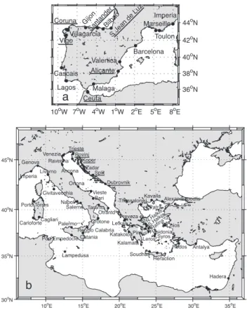
Hourly values from seventy three records covering the Mediterranean Sea and the Atlantic Iberian coasts have been

(4)

10oW 7oW 4oW 1oW 2oE 5oE 8oE 36oN 38oN 40oN 42oN 44oN

S.Jean de Luz Bilbao Santander Gijon Coruna Vigo Villagarcia Cascais Lagos Ceuta Malaga Alicante Valenica Barcelona Marseille Toulon Imperia

a

10oE 15oE 20oE 25oE 30oE 35oE 30o_N

35oN 40oN 45oN

Imperia

Genova II Livorno I Civitavecchia Napoli Salerno Palermo Port Empedocle Porto Torres Cagliari Carloforte Catania Reggio Calabria Crotone Taranto Otranto Bari Vieste Ortona Ravenna Venezia Trieste Koper Rovinj Zadar Split Dubrovnik Preveza Katakolon Kalamata Leros

Posidonia Syros

Thessaloniki Kavalla Alexandropoulis

Rodos Antalya

Hadera Heraclion Soudhas Lampedusa N.Halkis S.Halkis Ancona Pireus Lefkas

b

Patra Chios Rafina

Fig. 1. The location of the tide gauges used in this study. The geographical coordinates of the stations are given in Table 1. The underlined tide gauge stations are used in the analysis of the time series of percentiles.

few months to 68 years, and were found to be of varying quality. Extensive quality control was undertaken by Marcos et al. (2009). However further tests were run for this study in order to ensure the validity of extremes for all seasons. The tides were estimated and removed from the records on a yearly basis. Tidal constituents with a signal-to-noise ratio equal or larger than three were fitted to the time series by har-monic analysis using the standard programt-tide(Pawlowicz et al., 2002). The tidal record, built as the addition of the sig-nificant tidal components, has been used as a tool to identify temporal drifts in the original sea level observations. Where time shifts were identified the observed time series were re-tained for the analysis of extremes in observations but the segments were the time shifts were noted were rejected from the analysis of the tidal residuals.

2.2 Modelled sea level data

The meteorological contribution to sea level has been quanti-fied using the output of a barotropic oceanographic model. In the framework of the HIPOCAS (Hindcast of Dynamic Pro-cesses of the Ocean and Coastal Areas of Europe) project, atmospheric pressure and wind fields were produced by a dy-namical downscaling of the reanalysis of NCEP/NCAR for

the period 1958–2001 (Garc´ıa-Sotillo et al., 2005). These fields were used to force a barotropic version of the HAM-SOM (Hamburg Shelf Circulation Model) model covering the Mediterranean Sea and the Eastern Atlantic coast, with a spatial resolution of 1/4◦×1/6◦. The output was thus a consistent data set of 44 years of sea level hourly data (Rat-simandresy et al., 2008).

For each tide gauge station, data from the closest point of the hindcast grid has been subtracted from the obser-vations for the period covered by the model data (1958– 2001). The usefulness of this data set in reproducing the meteorologically-induced mean sea level has been proved in previous works (Tsimplis et al., 2005b; Gomis et al., 2006). The model is successful in reproducing changes in mean sea level but in general it underestimates the extremes.

The barotropic model is a better approximation of the di-rect atmospheric forcing than the standard inverse barometer correction in most places of the Mediterranean Sea and for high frequencies (Pascual et al., 2008). The inverse barom-eter correction assumes 1 cm of sea level increase(decrease) for 1 mbar reduction (increase) of local atmospheric pressure but it has been shown not to hold in the semi-enclosed seas and in particular in the Mediterranean. (e.g. Garrett and Ma-jaess, 1984).

2.3 Methodology

We assess changes in extreme sea level by determining changes in percentiles. The method is non parametric and only involves ranking the observations and looking at the value that correspond to a particular percentile.

The median corresponds to the 50th percentile and has been taken to be approximately the same as the mean value (Woodworth and Blackman, 2002, 2004). The case may be, for particular years, that the largest values do not correspond to extremes. This however is not a problem for the per-centiles method which are used here diagnostically for the existence of trends and not for return periods. We have cal-culated the percentiles on the basis of the available measure-ments ignoring the gaps in the time series. However gaps can be important in the estimation of percentiles either because an extreme is missed or because they occur in a particular period during which the mean sea level is high or low, thus affecting the estimation of the upper percentiles.

Percentiles are calculated for four seasons split as win-ter (December–March); spring (April–May); summer (June– September); and autumn (October–November). Trends for each season and the annual values are calculated for the 99.9%, 99% 95%, 90% and 50% percentiles. Here we re-port the results for 99.9%, 50% and 99.9%–50% values. The 99.9% corresponds to the highest value for the transitional seasons and to the top 3 values for the winter and summer that cover 4 months.

(5)

1940 1950 1960 1970 1980 1990 2000 Sjluz

Bilbao Santander

Santander 2 Gijon Coruna Coruna 2 Vigo Vigo 2 Villagarcia Cascais Lagos Ceuta Ceuta 2 Malaga Alica Valenica Barcelona Marsella Toulon Imperia Genova Livorno Civitavecchia Napoli Salerno Palermo Porto Empedocle Catania Reggio Crotone Taranto Otranto Bari Vieste Ortona Ancona Ravenna Venezia Trieste

Koper Rovinj Zadar Split Dubrovnik Preveza Lefkas Lefkas 2 Katakolon Kalamata Leros Posidonia Syros Pireus Rafina Patra North Halkis South Khalkis Thessaloniki Kavalla Alexandropoulis Alexandropoulis 2 Chios

Rodos Antalya Paphos Hadera Heraclion Soudhas Lampedusa Porto Torres Cagliari Carloforte

Year

Tide Gauges

Time Series of Hourly Tide Gauges

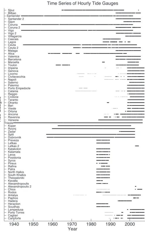
Fig. 2. Available hourly tide gauge observations. The thin lines indicate datum shifts within the time series records and consequently the record was split into more than one sub-records.

The latter are selected afresh after the tidal signal has been subtracted from the record. We also discuss extremes in the modelled sea level data and extremes for atmospherically corrected sea level values produced by subtracting the model values from the tidal residuals.

(6)

76 11 74 75 33 26 27 89 90 91 14 43 160

180 200 220 240 260 280

cm

Maximum Observations

Autumn Winter Spring Summer

76 11 74 75 33 26 27 89 90 91 14 43 0

20 40 60 80 100 120 140

Station Number

Maximum Tidal Residuals

76 11 74 75 33 26 27 89 90 91 14 43 0

20 40 60 80 100 120 140

cm

76 11 74 75 33 26 27 89 90 91 14 43 0

20 40 60 80 100 120 140

Atlantic Coasts

Station Number

Maximum HIPOCAS Observations Maximum Tidal Residuals minus

HIPOCAS Observations

a

b

c

d

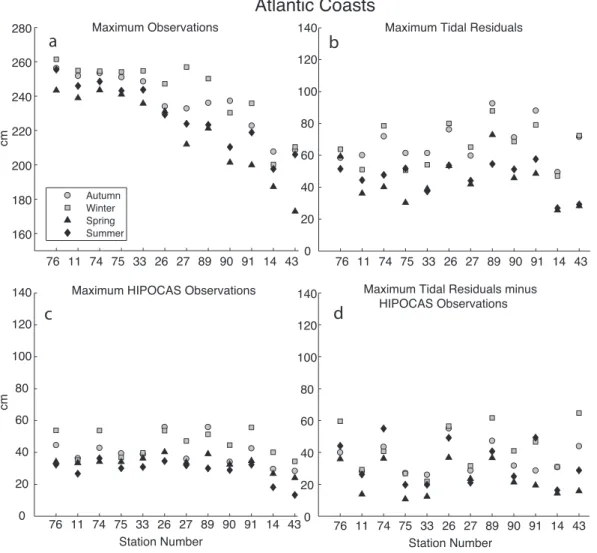
Fig. 3. Maximum seasonal values in the Atlantic coasts. Observations(a), tidal residuals(b), model(c)and tidal residual minus model values(d)for each season. The x-axis corresponds to the station number.

estimated the trends. Other methodologies exist for the esti-mation of trends in extremes. For example Katz and Brown (1992) have used a slope in a Generalised Extreme Value (GEV) distribution to assess trends and Barbosa (2008) has used quantile regression. We have used the GEV with a slope (Coles, 2001) to confirm the results obtained through the percentile method. The trends obtained by the two meth-ods were in agreement within their error bars. The percentile method was found to be more conservative in the sense that it produced fewer statistically significant trends than the GEV with a slope method.

The aim of our study is to describe the regional patterns of seasonal extremes and identify regional patterns of change in extreme. We start with a description of the maximum sea-sonal values as observed from the various time series. We use all the available data even if they consist of a few years. As a result in some stations there may not be data available for a particular season. However, the trends in the extremes are only estimated for the longest data sets (see Fig. 2).

(7)

3 Extreme sea levels

The various tide gauges span over different periods of time (Fig. 2). Thus it is possible that a tide gauge is in operation over a more energetic period of time while other tide gauges may not be operating during the same period. Nevertheless we consider instructive in starting our discussion of extremes by simply plotting the maximum value observed for each tide gauge in each season.

There is significant variance in observational extremes with values in the Atlantic exceeding 250 cm while in the Mediterranean are around 50–60 cm (Fig. 3a and Table 1). The spatial distribution of the observed maxima has been documented by Marcos et al. (2009). As expected the tidally dominated areas, the Atlantic coasts of the Iberian peninsula and the northern Adriatic Sea have the largest observed sea level values during the four seasons.

3.1 The Atlantic coasts

At the Atlantic coasts the observed maxima occur mainly in winter or, for a couple of stations (Vigo and Cascais) in au-tumn (Fig. 3a). Spring maxima are the lowest in all stations. The maximum observed values reduce by almost a meter as we move from the Bay of Biscay to Portugal and the southern coasts of Spain. The spatial distribution is primarily caused by the tides. This is demonstrated by examining the tidal residuals.

The maxima in the tidal residuals (Fig. 3b) do not show the same spatial pattern as shown by the observed maxima. They are highest at stations Vigo (no. 89) and Villagarcia (no. 91). The values of the maxima in the tidal residuals are less than half those of the maxima in the observations. Winter or autumn maxima values are the highest, with the predominant extreme occurring in autumn in most stations. Spring maxima are in most stations the smallest (Fig. 3b).

The model sea level values describe the contribution of at-mospheric pressure and wind. The maxima in these time se-ries (Fig. 3c) are between 20–60 cm. Winter maxima are the highest in most stations with autumn maxima values in gen-eral about 5 cm lower and summer maxima values being the lowest. However there are stations, for example Bilbao (11), Santander 2 (75) and Gijon (33) where no seasonal variation in the seasonal maxima can be identified.

The maxima in the atmospherically corrected values are generally lower than those of the maxima in the tidal residu-als (Fig. 3d). The seasonal spread of the maxima is in most stations reduced by the removal of the direct atmospheric ef-fects through the model. The range in the maxima is then only about 15–20 cm, consistent with an annual steric cy-cle of half that amplitude which is known to be the case for the Mediterranean (Tsimplis and Woodworth, 1995; Tsim-plis and Spencer, 1997; Marcos and TsimTsim-plis, 2007).

3.2 Western Mediterranean

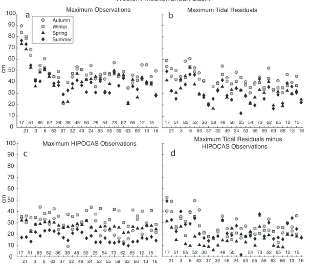
The maxima values for this region are shown in Fig. 4. The maxima are largest at the stations near the Strait of Gibral-tar but reduce at stations further inside the western Mediter-ranean Sea (Fig. 4a). The range of the maxima is between 55 cm in autumn to 20–30 cm for the maxima of summer or spring values.

The removal of the tidal signal reduces the maximum val-ues below 60 cm in all stations (Fig. 4b). The autumn max-ima remain the highest indicating that the contribution of the steric seasonal cycle is important. The range between the seasonal extremes is less than 20 cm in most stations.

The maxima in the model values are highest in winter for almost all stations apart from Valencia (no. 85) (Fig. 4c). The maxima in the spring values, when the seasonal cycle of the model peaks (Marcos and Tsimplis, 2007) are the second largest maxima. The summer season has the lowest maxima, around 10–15 cm at most stations.

The maxima in the atmospherically corrected sea level val-ues are up to 50 cm for the stations closest to the Strait of Gibraltar and reduce to 30 cm or less further in the western Mediterranean basin (Fig. 4d). Spring values are the lowest corresponding to the minimum of the steric cycle. The range of the seasonal maxima is now reduced to between 10 and 20 cm.

3.3 Eastern Mediterranean

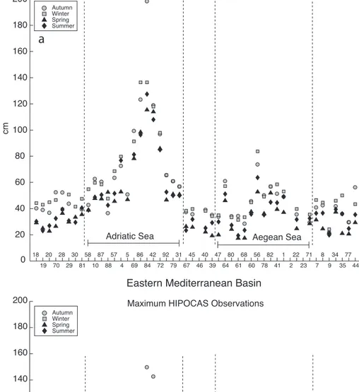
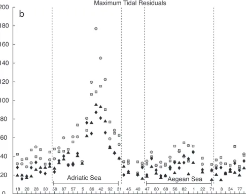
The spatial distribution of the maxima in the Eastern Mediterranean (Fig. 5) basin indicate two areas where the maxima are higher. The first is the Adriatic Sea where the maxima are higher than the rest of the eastern Mediterranean basin during all four seasons. The second area is the Aegean Sea where enhancement of the winter and autumn maxima is evident in the most northern stations but at a lesser extent than in the Adriatic Sea.

For the eastern Mediterranean five areas can be distin-guished. First the stations between the Strait of Sicily and the Strait of Otrando where maxima of around 50 cm occur either in winter or autumn. These are by 10–20 cm higher than the maxima in spring or summer.

Second the area in the Adriatic where the maxima reach almost 200 cm.

The third area is the Ionian Sea where the observed sea level maxima are less than 40 cm. In this area the larger max-ima occur in autumn or winter. The maxmax-ima for summer and spring are as small as 20 cm.

(8)

17 21

51 3

85 6

52 83

36 37

38 32

48 49

50 24

25 53

54 55

73 59

62 63

65 66

12 13

15 16

0 10 20 30 40 50 60 70 80 90 100

Station Number

cm

17 51 85 52 36 38 48 50 25 54 73 62 65 12 15 21 3 6 83 37 32 49 24 53 55 59 63 66 13 16

0 10 20 30 40 50 60 70 80 90 100

cm

Maximum HIPOCAS Observations

17 51 85 52 36 38 48 50 25 54 73 62 65 12 15 21 3 6 83 37 32 49 24 53 55 59 63 66 13 16

Maximum Tidal Residuals minus HIPOCAS Observations

17 51 85 52 36 48 50 54 73 62 65 12 15

Station Number

21 3 6 83 37 32 49 24 53 55 59 63 66 13 16 Western Mediterranean Basin

a

b

c

d

Fig. 4.As Fig. 3 for the western Mediterranean tide-gauges.

The removal of the tidal signal, which is generally small, apart from the Adriatic Sea and the station of North Halkis reduces the maxima in some of the stations The values of extremes in the Aegean Sea and the eastern Mediterranean appear now more spatially consistent (Fig. 5b). In the Adri-atic Sea maxima values of up to 180 cm in autumn occur. The winter maxima are significantly smaller by around 40– 50 cm. The spread between seasonal maxima in the other areas of the eastern Mediterranean is around 20 cm.

The model maxima (Fig. 5c) occur in winter in all areas and reach up to 45 cm apart from the north Adriatic stations where the maxima occur in autumn and reach 150 cm. The other seasons show values smaller by 10–20 cm, the summer maxima being the lowest.

The maxima in the atmospherically corrected time series are smaller than the maxima in the tidal residuals in all ar-eas (Fig. 5d). Maxima in the atmospherically corrected time series are around 30 cm for winter and autumn and less than 20 cm, in some cases less than 10 cm in spring. Notably the pattern in the Adriatic Sea of the very high maxima found in the observations and in the tidal residuals still occurs in

the atmospherically corrected maxima. This indicates that factors other than those described and modeled here con-tribute to the creation of maxima. It is possible that the discrepancy is due to the unsatisfactory resolution of local winds as suggested by Wakelin et al. (1999) and Wakelin and Proctor (2002) and to the basin resonance of the Adri-atic Sea not correctly resolved by the model. However note that the barotropic model used here is forced by downscaled atmospheric parameters while those studied by Wakelin et al. (1999) and Wakelin and Proctor (2002) were not using downscaled atmospheric forcing.

4 Trends in extreme sea levels

(9)

18 19

20 70

28 29

30 81

58 10

87 88

57 4

5 69

86 84

42 72

92 79

31 67

45 46

40 39

47 64

80 61

68 60

56 78

82 41

1 2

22 23

71 7

8 9

34 35

77 44 20

40 60 80 100 120 140 160 180 200

cm

Eastern Mediterranean Basin

Adriatic Sea Aegean Sea

0

a

19 70 29 81 10 88 4 69 84 72 79 67 46 39 64 61 60 78 41 2 23 6 8 35 44 0

20 40 60 80 100 120 140 160 180 200

cm

18 20 28 30 58 87 57 5 86 42 92 31 45 40 47 80 68 56 82 1 22 71 7 34 77 Adriatic Sea

Eastern Mediterranean Basin

Aegean Sea Maximum HIPOCAS Observations

Fig. 5.As Fig. 3 for the eastern Mediterranean tide-gauges.

The trends in the 99.9% percentile of the observed val-ues are mostly positive (Table 2). In the Atlantic coasts, the strongest positive trends are found for autumn and the

(10)

Station Number

19 70 29 81 10 88 4 69 84 72 79 67 46 39 64 61 60 78 41 2 23 7 9 35 44 0

20 40 60 80 100 120 140 160 180 200

cm

Adriatic Sea

18 20 28 30 58 87 57 5 86 42 92 31 45 40 47 80 68 56 82 1 22 71 8 34 77 Aegean Sea

b

19 70 29 81 10 88 4 69 84 72 79 67 46 39 64 61 60 78 41 2 23 6 8 35 44 0

20 40 60 80 100 120 140 160 180 200

Station Number

cm

Maximum Tidal Residual minus HIPOCAS Observations

Adriatic Sea

18 20 28 30 58 87 57 5 86 42 92 31 45 40 47 80 68 56 82 1 22 71 7 34 77 Aegean Sea

Fig. 5.Continued.

the Adriatic Sea the highest trends in the 99.9 percentile of the observed values are found in the spring, one of the peri-ods where the occurring extreme values are low in compari-son with other seacompari-sons.

(11)

−6 −4 −2 0 2 4 6

mm/yr

76 74 26 89 17 3 84 42 72 79 31 −6

−4 −2 0 2 4 6

mm/yr

76 74 26 89 17 3 84 42 72 79 31 Station Number

76 74 26 89 17 3 84 42 72 79 31 Station Number @ 99.9 Percentile @ 50 Percentile

@ 99.9 Percentile @ 50 Percentile

Observations

Residuals Autumn

Winter Spring Summer

Atlantic Coasts

Adriatic Sea

W

e

st

ern

M

edit

erranean

Atlantic Coasts

Adriatic Sea

W

e

st

ern

M

edit

erranean

Atlantic Coasts

Adriatic Sea

W

e

st

ern

M

edit

erranean

Atlantic Coasts

Adriatic Sea Atlantic Coasts

Adriatic Sea

Atlantic Coasts

Adriatic Sea

(a) (b) (c)

(d) (e) _(f)

W

e

st

ern

M

edit

erranean

W

e

st

ern

M

edit

erranean

W

e

st

ern

M

edit

erranean

@ 99.9 − 50 Percentile

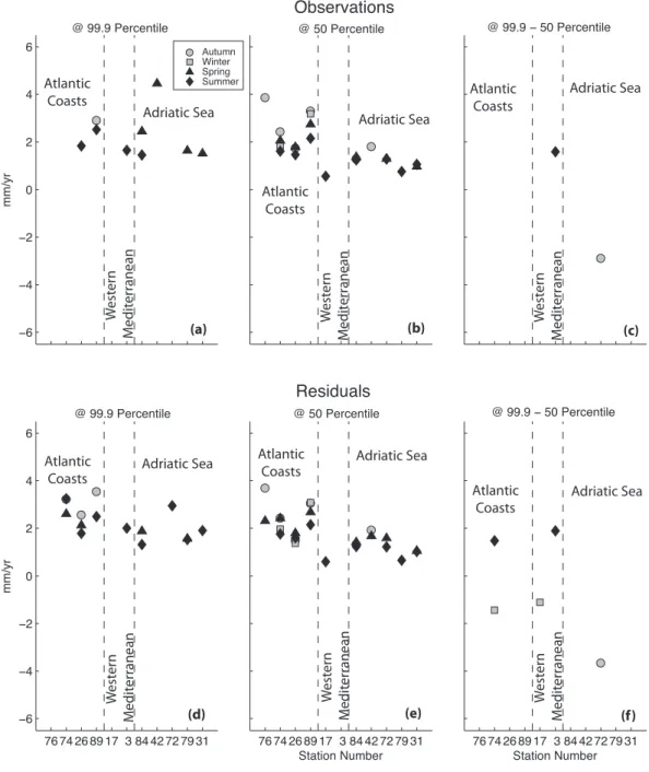
Fig. 6. Significant trends in the 99.9 and 50 percentiles and their differences. (a–c)for the observed values;(d–f)for the tidal residuals; (g–i)for the model values;(j–l)for the corrected by the model tidal residuals.

having small positive trends. When the observed trends of the 99.9%–50% are calculated (Table 2) most trends in all seasons fall within±0.5 mm/yr with a (not statistically sig-nificant) tendency for the Atlantic stations to show small neg-ative trends. This means that for the Atlantic the increases in the mean are slightly higher than the increases in the 99.9%. The most remarkable changes occur at stations Koper (42) and Rovinj (72) where autumn values show significantly neg-ative trends. Taking into account that for the Adriatic autumn shows maxima values, this is a positive, from the point of view of coastal protection, development. Notably in Koper

(42) it appears that the winter and spring extremes have been increasing in time.

(12)

0 2 4 6

mm

/yr

76 74 26 89 17 3 84 42 72 79 31 0

2 4 6

mm

/yr

76 74 26 89 17 3 84 42 72 79 31 76 74 26 89 17 3 84 42 72 79 31

HIPOCAS

Residuals-HIPOCAS Atlantic

Coasts

Adriatic Sea

W

e

st

ern

M

edit

erranean

Atlantic Coasts

Adriatic Sea

W

e

st

ern

M

edit

erranean

Atlantic Coasts

Adriatic Sea

W

e

st

ern

M

edit

erranean

W

e

st

ern

M

edit

erranean

W

e

st

ern

M

edit

erranean

W

e

st

ern

M

edit

erranean

(g) (h) (i)

(j) (k) (l)

Atlantic Coasts

Adriatic Sea Atlantic Coasts

Adriatic Sea

Fig. 6.Continued.

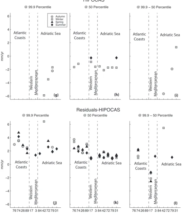
The modeled sea level data are less noisy than observa-tions and as a consequence the estimated trends of the 99.9% and 50% are more consistent (Fig. 6g, h, i). Starting from the 50% (Fig. 6h) negative mean sea level trends are found with very small positive trends in spring and no trends in the median values in the other seasons.

The 99.9% percentiles show in the Atlantic positive trends in summer and negative trends in winter in many stations and positive trends but in fewer stations in autumn (Fig. 6g). Small negative trends are found in the 99.9% for all sea-sons in the western Mediterranean Sea. The stations of the

Adriatic Sea show significant reductions (4–6 mm/yr) in the 99.9% in autumn and winter and almost no change in spring and summer.

The 99.9%–50% trends are significant in the Adriatic in winter and autumn. These are negative indicating reduction of wind and or increases of maxima of atmospheric pressure (Fig. 6i). Positive trends in summer are found in the Atlantic sector with negative trends in autumn and spring in some of the stations.

(13)

Table 2. Seasonal trends for the 99.9 percentile, the 50 percentile and the 99.9–50 percentile in mm/yr. There are four columns for each season that correspond to the trend estimated from tide gauge observations, tidal residuals, the model values (HIPOCAS) and the tide residuals minus HIPOCAS, respectively. Note, that because HIPOCAS covers the period 1958 and 2001, the trend estimates at the fourth column of each season only covers the overlapping period between HIPOCAS data and the corresponding tide-gauge record. The error bars are those of the linear fit at the 95% level of significance.

Autumn @ 99.9% Winter @ 99.9%

Station name Period Obs Tide Res Hip Hip-Res Obs Tide-Res Hip Hip-Res

3 Alicante 1957 1997 0.3±1.5 0.0±1.7 −0.7±1.4 −0.3±1.4 −0.6±1.9 −0.9±2.0 −1.3±1.4 0.0±1.3

17 Ceuta 1944 2002 −0.1±1.2 0.6±1.2 −0.7±1.6 −0.4±1.3 0.0±1.1 −1.0±1.4 −1.0±1.5 −1.2±2.2

26 Coruna 1943 2000 1.6±2.3 2.6±1.9 0.0±2.4 2.7±2.1 0.4±2.1 0.9±2.1 −1.0±2.1 1.6±2.0

31 Dubrovnik 1956 2001 0.4±1.5 0.5±1.6 −1.0±1.2 1.1±1.5 −0.6±1.6 −0.1±2.1 −0.4±1.4 0.6±1.7

42 Koper 1962 1999 −1.0±4.0 −1.2±6.6 −5.7±5.9 0.9±5.2 1.8±3.3 3.0±4.2 −5.9±4.0 6.4±5.2

72 Rovinj 1959 2001 −2.0±2.9 −2.8±4.4 −4.0±4.2 −0.0±3.6 −0.3±2.4 0.7±3.2 −3.5_±3.2 3.9±3.9

74 Santander 1943 2000 2.9±3.0 3.2±1.7 −0.9±1.8 3.5±1.7 0.7±1.9 0.5±1.9 −1.1±1.6 3.6±1.5

76 Sjluz 1964 2003 2.5±6.4 2.2±4.4 −1.2±2.7 3.0±2.5 1.3±4.3 0.1±3.9 −1.4±2.5 1.8±3.3

79 Split 1956 2001 −0.3±1.7 0.2±2.3 −2.2±2.0 2.6±2.1 −0.1±1.6 −0.5±2.3 −1.7±1.5 0.9±2.1

84 Trieste 1939 2005 0.6±2.7 2.1±3.6 −4.4±4.8 −2.3±5.2 1.4±1.8 1.5±2.0 −3.5±3.9 1.5±4.2

89 Vigo 1943 2000 2.9±2.4 3.6±2.1 0.1±2.3 2.5±2.2 1.7±2.0 2.2±2.2 −1.1±2.1 2.0±2.1

Autumn @ 50% Winter @ 50%

Station name Period Obs Tide Res Hip Res-Hip Obs Tide-Res Hip Res-Hip

3 Alicante 1957 1997 −0.5±1.0 −0.5±1.1 −0.4±0.8 0.5±0.6 −1.1±1.5 −1.1±1.5 −1.6±0.9 0.3±0.7

17 Ceuta 1944 2002 0.5±0.7 0.5±0.7 −0.5±0.5 1.0±0.8 0.1±0.6 0.1±0.6 −0.9±0.6 0.9±0.7

26 Coruna 1943 2000 1.8±1.1 1.5±1.1 −0.1±1.0 1.7±1.1 1.2±1.2 1.4±1.3 −1.0±1.2 1.7±1.2

31 Dubrovnik 1956 2001 0.8±1.3 0.8±1.4 −0.2±0.8 1.3±0.8 −0.6±1.3 −0.6±1.3 −1.7±1.0 1.0±0.7

42 Koper 1962 1999 1.8±1.8 1.9±1.8 −0.1±1.2 1.9±0.9 −0.9±1.7 −1.2±1.8 −2.1±1.3 1.0±0.9

72 Rovinj 1959 2001 0.9±1.4 0.9±1.5 −0.3±1.0 1.2±0.7 −0.5±1.7 −0.7±1.7 −1.7±1.1 1.2±0.9

74 Santander 1943 2000 2.4_±1.0 2.4_±1.1 ₋0.2±1.0 2.3_±1.2 1.8_±1.1 2.0_±1.2 ₋1.2_±1.1 2.6_±1.0

76 Sjluz 1964 2003 3.9±2.7 3.7±2.8 0.1±1.2 3.7±1.8 1.4±2.1 1.8±2.2 −1.7±1.6 3.4±1.5

79 Split 1956 2001 0.6±1.4 0.6±1.5 −0.3±0.9 0.9±0.8 −0.9±1.4 −0.9±1.4 −1.7±1.0 0.4±0.8

84 Trieste 1939 2005 1.3±0.8 1.3±0.8 −0.3±1.0 1.3±0.8 0.7±0.8 0.6±0.8 −1.5±1.1 1.1±0.7

89 Vigo 1943 2000 3.3±1.1 3.1±1.1 −0.1±1.0 3.0±1.3 3.2±1.2 3.1±1.2 −1.1±1.1 3.1±1.3

Autumn @ 99.9%–50% Winter @ 99.9%–50%

Station name Period Obs Tide Res Hip Hip-Res Obs Tide-Res Hip Hip-Res

3 Alicante 1957 1997 0.8±1.5 0.5±1.7 −0.3±1.2 −0.8±1.3 0.5±1.5 0.2±1.5 0.3±1.3 −0.3±1.1

17 Ceuta 1944 2002 −0.6±1.0 0.1±1.0 −0.2±1.5 −1.3±1.2 −0.1±0.7 −1.1±1.1 −0.2±1.3 −2.1±1.9

26 Coruna 1943 2000 −0.1±1.9 1.1±1.5 0.1±2.2 1.0±1.8 −0.8±1.6 −0.4±1.6 0.1±2.0 −0.2±1.6

31 Dubrovnik 1956 2001 −0.4±1.5 −0.4±1.6 −0.8±1.3 −0.2±1.2 −0.0±1.3 0.5±1.7 1.3±1.3 −0.3±1.3

42 Koper 1962 1999 −2.8±3.6 −3.1±5.6 −5.7_±5.4 ₋0.9±4.8 2.7±3.0 4.2±4.3 −3.8±4.1 5.5_±5.2

72 Rovinj 1959 2001 −2.9±2.6 −3.7±3.6 −3.6±3.8 −1.3±3.3 0.2±2.0 1.4±3.1 −1.8±3.1 2.7±3.9

74 Santander 1943 2000 0.5±2.8 0.8±1.2 −0.7±1.5 1.2±1.2 −1.1±1.6 −1.4±1.4 0.1±1.7 1.0±1.0

76 Sjluz 1964 2003 −1.4±5.4 −1.5±3.1 −1.3±2.2 −0.7±1.6 −0.0±3.6 −1.7±3.5 0.2±2.9 −1.6±2.9

79 Split 1956 2001 −0.8±1.4 −0.4±1.8 −1.9±1.9 1.6±1.8 0.8±1.3 0.4±1.9 0.0±1.5 0.5±2.0

84 Trieste 1939 2005 −0.7±2.5 0.7±3.3 −4.1±4.4 −3.6±5.0 0.8±1.5 1.0±1.8 −1.9±3.9 0.4±4.2

89 Vigo 1943 2000 −0.4±1.9 0.5±1.6 0.3±2.2 −0.5±1.6 −1.5±1.6 −0.9±1.7 −0.1±1.9 −1.1±1.8

In addition although the spread of seasonal trends is reduced in relation to that of the trends in the 99.9% of the obser-vations the difference in the trends between stations appear increased (Fig. 6j).

By contrast the 50% of the atmospherically corrected trends are much more spatially consistent than the trends in the 50% of either the observations or the tidal residuals. Positive trends of around 3 mm/yr in the Atlantic and about

1.7 mm/yr in the Adriatic Sea and with very little difference seasonally (Fig. 6k) are found. Smaller values, less than 1 mm/yr, are found in the western Mediterranean.

(14)

Table 2.Continued.

Spring @ 99.9% Summer @ 99.9%

3 Alicante 1957 1997 −0.1±1.6 −0.6±1.7 −0.3±1.1 1.1±1.6 1.6±1.4 2.0±1.4 −0.3±0.7 1.4±1.3

17 Ceuta 1944 2002 0.3±1.1 0.2±1.2 −0.7±1.2 −1.6±1.7 0.7±0.8 0.7±0.8 −0.4±0.5 −0.4±1.4

26 Coruna 1943 2000 1.0±2.5 2.1±1.5 −0.5±1.7 2.9±1.4 1.8±1.7 1.8±1.2 0.7±1.5 1.1±1.8

31 Dubrovnik 1956 2001 1.5_±1.4 0.9±1.4 0.1±1.2 0.9±1.2 0.9±1.2 1.9_±1.2 ₋0.6±0.8 2.3_±1.3

42 Koper 1962 1999 4.5±3.9 0.9±4.4 0.4±2.7 −0.2±3.8 1.0±2.2 2.0±3.2 0.5±1.4 1.1±3.0

72 Rovinj 1959 2001 2.3±2.7 1.8±3.0 0.7±2.0 3.5±2.4 1.1±1.9 3.0±2.4 0.1±1.1 2.6±2.3

74 Santander 1943 2000 2.0±2.7 2.6±1.3 0.6±1.4 4.7±1.7 1.4±2.1 3.2±1.2 0.9±1.5 4.2±1.6

76 Sjluz 1964 2003 −0.6±6.1 2.0±4.0 1.5±1.9 1.4±3.2 0.5±4.5 −0.0±2.7 1.6±1.9 0.3±2.2

79 Split 1956 2001 1.6±1.5 1.6±1.5 −0.0±1.6 2.0±1.3 0.6±1.2 1.5±1.3 −0.6±1.0 1.9±1.0

84 Trieste 1939 2005 2.5±1.6 1.9±1.7 0.3±2.3 0.8±2.3 1.5±1.1 1.3±1.2 0.2±1.2 1.6±1.5

89 Vigo 1943 2000 1.4±2.3 1.5±1.8 −0.6±1.7 1.7±1.4 2.5±1.8 2.5±1.4 0.5±1.4 2.3±1.5

Spring @ 50% Summer @ 50%

3 Alicante 1957 1997 0.7±0.7 0.7±0.7 0.3±0.6 0.4±0.5 0.1±0.5 0.1±0.5 −0.2±0.3 0.2±0.4

17 Ceuta 1944 2002 0.5±0.7 0.6±0.7 −0.1±0.4 1.0±1.0 0.6±0.5 0.6±0.5 −0.3±0.2 0.8±0.8

26 Coruna 1943 2000 1.8±0.9 1.8±0.8 0.8±0.8 2.2±0.8 1.5±0.7 1.6±0.6 0.1±0.3 2.2±0.8

31 Dubrovnik 1956 2001 1.0±0.9 1.0±0.9 −0.5±0.5 1.4±0.8 1.1±0.6 1.0±0.6 −0.2±0.2 1.2±0.6

42 Koper 1962 1999 1.4±1.4 1.7_±1.4 ₋0.1±0.8 1.8_±1.0 0.9±0.9 0.7±0.8 −0.2±0.3 1.0_±0.8

72 Rovinj 1959 2001 1.3±1.0 1.6±1.1 −0.2±0.6 1.6±0.8 1.3±0.8 1.2±0.8 −0.1±0.3 1.4±0.8

74 Santander 1943 2000 2.1±1.0 2.4±0.9 0.5±0.7 2.7±1.0 1.6±0.6 1.8±0.6 −0.0±0.3 2.0±0.8

76 Sjluz 1964 2003 2.1±2.4 2.3±2.3 −0.1±1.0 2.4±1.8 1.2±1.4 1.1±1.4 0.0±0.4 1.2±1.4

79 Split 1956 2001 0.7±0.9 0.7±0.9 −0.2±0.5 1.0±0.7 0.7±0.5 0.7±0.5 −0.2±0.2 0.8±0.5

84 Trieste 1939 2005 1.4_±0.6 1.4_±0.5 ₋0.2±0.6 1.4_±0.7 1.2_±0.3 1.2_±0.3 ₋0.1±0.2 1.2_±0.5

89 Vigo 1943 2000 2.7±0.9 2.7±0.9 0.7±0.8 2.6±1.1 2.2±0.7 2.1±0.7 0.1±0.2 1.7±1.1

Spring @ 99.9%–50% Summer @ 99.9%–50%

3 Alicante 1957 1997 −0.7±1.6 −1.3±1.7 −0.6±1.2 0.6±1.6 1.6±1.3 1.9±1.3 −0.2±0.7 1.2±1.2

17 Ceuta 1944 2002 −0.1±0.9 −0.4±1.1 −0.6±1.1 −2.6±1.5 0.1±0.7 0.1±0.7 −0.2±0.5 −1.2±1.1

26 Coruna 1943 2000 −0.8±2.5 0.3±1.2 −1.3±1.7 0.7±1.2 0.4±1.6 0.2±1.2 0.6±1.4 −1.1±1.8

31 Dubrovnik 1956 2001 0.5±1.3 −0.2±1.3 0.6±1.3 −0.5±1.1 −0.1±1.0 0.9±1.1 −0.3±0.9 1.1±1.2

42 Koper 1962 1999 3.0±3.7 −0.8±4.4 0.5±2.9 −2.0±3.7 0.1±2.0 1.3±2.9 0.7±1.4 0.1±2.6

72 Rovinj 1959 2001 1.0±2.4 0.2±2.8 0.9±2.2 1.9±2.1 −0.2±1.8 1.7±2.1 0.2±1.1 1.2±1.9

74 Santander 1943 2000 −0.0±2.6 0.2±1.0 0.1±1.3 2.1±1.3 −0.2±2.0 1.5±1.0 0.9±1.4 2.2±1.4

76 Sjluz 1964 2003 −2.7±5.9 −0.3±3.5 1.6±2.0 −1.0±2.5 −0.6±4.2 −1.1±2.5 1.5±1.9 −0.9±2.0

79 Split 1956 2001 0.9±1.4 0.9±1.3 0.2±1.6 1.0±1.2 −0.2±1.0 0.9±1.2 −0.4±1.1 1.1±0.9

84 Trieste 1939 2005 1.1±1.5 0.5±1.6 0.5±2.5 −0.6±2.2 0.2±1.0 0.1±1.1 0.3±1.2 0.4±1.4

89 Vigo 1943 2000 −1.3±2.3 −1.2±1.8 −1.4±1.6 −1.0±1.5 0.4±1.6 0.4±1.1 0.4±1.4 0.6±1.1

the values become too large. The reason why the trends in the 99.9% of the atmospherically corrected time series be-come spatially inconsistent is unknown. We speculate that the model has spatially variable skill in estimating extremes and this results into the diversity of the trends.

To assess the effect of the existing gaps in the tide-gauge records on the estimation of trends we have redone the anal-ysis of extremes in the model data for the whole period cov-ered by each tide-gauge but including all values for that pe-riod. We compared these results with the earlier described results where the trends were estimated for only the periods coinciding with those in which the tide-gauges had data and we found no significant differences in the derived trends.

5 Correlation with atmospheric patterns

It is well established that interannual variability within the Mediterranean Sea especially in the winter is significantly correlated with the North Atlantic Oscillation (see for exam-ple Tsimplis and Josey, 2001; Gomis et al., 2006). In addi-tion significant sea level change over several decades have been driven by changes in the NAO (Tsimplis and Josey, 2001).

(15)

−1 −0.8 −0.6 −0.4 −0.2 0 0.2 0.4 0.6 0.8 1

Observations

C

o

rr

elation

76 74 26 89 17 3 84 42 72 79 31 76 74 26 89 17 3 84 42 72 79 31 Station Number

76 74 26 89 17 3 84 42 72 79 31 Station Number

Adriatic Sea Atlantic

Coasts

W

est

ern

M

edit

erranean Adriatic Sea Atlantic

Coasts

W

est

ern

M

edit

Coasts

W

est

ern

M

edit

erranean

Coasts

W

est

ern

M

edit

Coasts

W

est

ern

M

edit

Coasts _West

ern

M

edit

erranean

(a) (b) (c)

(d) (e) (f)

Station Number

Tidal Residuals

−1 −0.8 −0.6 −0.4 −0.2 0 0.2 0.4 0.6 0.8 1

C

o

rr

elation

(g) (h) (i)

−1 −0.8 −0.6 −0.4 −0.2 0 0.2 0.4 0.6 0.8 1

C

o

rr

elation

HIPOCAS @ 99.9 - 50 Percentile

@ 99.9 - 50 Percentile @ 99.9 - 50 Percentile

Coasts

W

est

ern

M

edit

Coasts

W

est

ern

M

edit

erranean Atlantic _{Adriatic Sea}

Coasts _West

ern

M

edit

erranean

Fig. 7. Seasonal correlations of the NAO index with the 99.9 percentile, 50 percentile and their difference. (a–c)for the observed values; (d–f)for the tidal residuals;(g–i)for the model values. Each of the seasonal correlation coefficients has an associated value in order to be significant at 95% level. We have plotted the highest of the four values as giving the most conservative estimate for the level of significance.

Figure 7 shows the correlation coefficients for seasonal NAO values with the corresponding seasonal sea level per-centiles. For the sea level observations the negative corre-lations are higher for winter both at 99.9% and at 50%. In addition significant negative correlations are found for

(16)

76 74 26 89 17 3 84 42 72 79 31 76 74 26 89 17 3 84 42 72 79 31 Station Number

76 74 26 89 17 3 84 42 72 79 31 Station Number Station Number

Observations

@ 99.9 - 50 Percentile

Autumn Winter Spring Summer Adriatic Sea Atlantic Coasts W est ern M edit

erranean Adriatic Sea Atlantic Coasts W est ern M edit

erranean Adriatic Sea Atlantic Coasts W est ern M edit erranean

Tidal Residuals

@ 99.9 - 50 Percentile

Adriatic Sea Atlantic Coasts W est ern M edit

erranean Adriatic Sea Atlantic Coasts W est ern M edit

Coasts _West

ern

M

edit

erranean

(a) _(b) (c)

(d) _(e) (f)

HIPOCAS @ 99.9 - 50 Percentile

Adriatic Sea Atlantic Coasts W est ern M edit erranean Adriatic Sea Atlantic Coasts W est ern M edit erranean Adriatic Sea Atlantic Coasts W est ern M edit erranean (g) (h) (i) −1 −0.8 −0.6 −0.4 −0.2 0 0.2 0.4 0.6 0.8 1 C o rr elation −1 −0.8 −0.6 −0.4 −0.2 0 0.2 0.4 0.6 0.8 1 C o rr elation −1 −0.8 −0.6 −0.4 −0.2 0 0.2 0.4 0.6 0.8 1 C o rr elation

Fig. 8. Seasonal correlations of the MOI index with the 99.9 percentile, 50 percentile and their difference. (a–c)for the observed values; (d–f)for the tidal residuals;(g–i)for the model values. Each of the seasonal correlation coefficients has an associated value in order to be significant at 95% level. We have plotted the highest of the four values as giving the most conservative estimate for the level of significance.

between the NAO and the 99.9% percentile becomes statisti-cally insignificant when the 50% is subtracted (Fig. 7c). Thus the influence of the NAO at the 99.9% is due to the changes in mean sea level.

The subtraction of the tidal signal does not significantly change the above results in respect of the 99.9% percentile

except in the Adriatic (Fig. 7d, e, f) where the 99.9% cor-relations with the winter NAO in the Adriatic Sea are much smaller than the correlations between the NAO index and the 99.9% percentile of the observations.

(17)

found between the NAO and the observations. Thus only in a few stations in the winter the correlation is statistically signif-icant (Fig. 7g). By contrast for the 50% percentile signifsignif-icant negative correlation with the NAO is found for all seasons for stations at the Atlantic and the western Mediterranean (ex-cept Ceuta in the summer) (Fig. 7h). The 99.9%–50% is not statistically significantly correlated with the NAO. In some of the stations the significant correlation of the NAO with the 50% comes through as positive correlation of the 99.9%– 50% with the NAO. When the model data are subtracted from the tidal residuals most correlations with the NAO and the MOI become statistically insignificant at the 99.9%, the 50% percentiles and the 99.9%–50% (not shown). Exceptions are the winter and autumn values of the 50% percentile at Split and Dubrovnik when correlated with the MOI.

The same patterns but with higher correlations are found if the (inverted) Mediterranean Oscillation Index (MOI) is used instead of the NAO (Fig. 8). The MOI used here comes from Suselj et al. (2008). Tsimplis and Shaw (2008) have identified that mean sea level is better correlated with the (inversed) MOI rather than the NAO but here this better cor-relation is shown to be present in the 99.9% too, especially during autumn. However, again only a few correlation val-ues remain statistical significant after the deduction of the median value (Fig. 8c, f, i).

The correlation of the sea level extremes with the large scale atmospheric patterns indicate that the atmospheric con-tribution causes most of the observed extremes and their changes Moreover these changes are linked with changes in the 50% percentile. The correlation of the NAO and the MOI is stronger for the 50% for the model values rather than the observations, an expected result probably because the noise level is much lower in the model. However, with respect to the 99.9% percentile the correlation with the NAO is stronger with the observations than with the model while the opposite is true for the MOI. We do not understand the reason for this.

6 Summary and conclusions

An extensive dataset of hourly sea level values from tide gauges and the output of a barotropic model have been anal-ysed in respect of seasonal extreme values. Significant spa-tial variability in the observed maxima is identified in all seasons. In respect of the Atlantic stations this is primar-ily due to the varying tidal signal. When the tidal signal is removed most of the Atlantic stations show maxima of less than 90 cm occurring in winter or autumn and maxima in spring and summer lower than 60 cm. The wind and at-mospheric forcing contributes, according to the barotropic model used, about 50 cm in the winter maxima and between 20–40 cm in the maxima of the other seasons.

In the western Mediterranean Sea the maxima in the ob-served values are less than 50 cm, except near the Strait of Gibraltar where they reach values of round 90 cm. Direct

atmospheric forcing contributes significantly in the maxima and in several stations its contribution is around 45 cm during winter and between 10–20 cm during summer.

The Adriatic Sea provides the most interesting area for the spatial variability of sea level maxima with the northern-most stations showing the largest maxima. This behaviour is partly due to the direct atmospheric forcing contribution which also shows significant increases at the northern sta-tions of the Adriatic. It is also well established that the tidal signal is increasing significantly at the northern parts of the Adriatic basin (Tsimplis et al., 1995).

The time series corrected for the tidal signal and for the direct atmospheric forcing contribution through the use of the barotropic model show a reduction in the size of the ex-tremes in all seasons. However in the north of the Adriatic Sea the same spatial pattern exists and the extremes in the residual still increase towards the north part of the basin. Sea level extremes in the northern Adriatic are affected by a res-onant oscillation of around 21.5 h excited by the local wind field (Cerovecki et al., 1997; Raicich, 1999; Vilibic, 2006). If the barotropic model of the direct atmospheric effects was successful in modeling the atmospherically driven sea level component then the atmospherically corrected values would not have the increased values towards the northern Adriatic. Thus it is our view that the model does not represent the extreme values with sufficient accuracy either because the bathymetry in the model is not capable of creating the reso-nance or because the local wind field is not represented ac-curately enough. The latter problem is a general problem for models in the area (Wakelin and Proctor, 2002) but the persistence of the problem with the model used in this case means that the introduction of atmospheric downscaling is not capable of representing the local winds in the Adriatic.

Trends in the 99.9% percentiles are found at various sea level records for the winter and the autumn seasons. How-ever the trends in the 99.9%–50% percentile are not signifi-cant. This suggests that the trends in the 99.9% percentile are in line with mean sea level changes. The North Atlantic Os-cillation Index and the Mediterranean OsOs-cillation Index are well correlated with the changes in the 99.9% winter values in the Atlantic, western Mediterranean and the Adriatic sta-tions and, in the Atlantic and western Mediterranean in the autumn too. The correlation becomes insignificant when the 50% is removed.

(18)

Thus, no seasonal changes in extremes in addition to those in the median are detectable. Furthermore, we have mapped the spatial patterns of seasonal extremes for the Mediterranean and the Atlantic coasts of the Iberian peninsula.

The results of this work will contribute in assessing future changes in sea level extremes in models. This work provides guidance on the seasonal and spatial patterns of extremes in the Mediterranean over the past decades. Of course signif-icant gaps that exist in the observational records may partly bias the results. However it is arguable that the seasonal and spatial patterns of models that include the sea level parameter need to be matched, even if only in broad terms, to the results presented here. In addition the seasonal patterns emerging in-dicate that future changes must also be assessed on the basis of seasonal analysis in order to be able to identify whether the changes in extremes will be seasonally biased.

Acknowledgements. This work was performed as part of the EC program CIRCE. We are grateful to Marta Marcos for her assistance.

Edited by: U. Ulbrich

Reviewed by: three anonymous referees

References

Barbosa, S. M.: Quantile trends in Baltic sea level, Geophys. Res. Lett., 35, L22704, doi:10.1029/2008GL035182, 2008.

Cazenave, A., Bonnefond, P., Mercier, F., Dominh, K., and Touma-zou, V.: Sea level variations in the Mediterranean Sea and Black Sea from satellite altimetry and tide gauges, Global Planet. Change, 34, 59–86, 2002.

Cazenave, A., Cabanes, C., Dominh, K., and Mangiarotti, S.: Re-cent Sea Level Change in the Mediterranean Sea Revealed by Topex/Poseidon Satellite Altimetry, Geophys. Res. Lett., 28, 1607–1610, 2001.

Cerovecki, I., Orlic, M., and Hendershott, M. C.:, Adriatic seiche decay and energy loss to the Mediterranean, Deep-Sea Res., PART I-OCEANOGRAPHIC RESEARCH PAPERS, 44(12), 2007–2029, 1997.

Coles, S.: An introduction to statistical modeling of ExtremeVal-ues., Springer-Verlag London Limited., 208 pp., 2001.

Fenoglio-Marc, L.: Long-term sea level change in the Mediter-ranean Sea from multi-satellite altimetry and tide gauges, Phys. Chem. Earth, 27, 1419–1431, 2002.

Garc´ıa-Sotillo, M., Ratsimandresy, A. W., Carretero, J. C., Ben-tamy, A., Valero, F., and Gonz´alez-Rouco, F.: A high-resolution 44-year atmospheric hindcast for the Mediterranean Basin: con-tribution to the regional improvement of global reanalysis, Clim. Dynam., 25(2–3), 219–236, doi:10.1007/s00382-005-0030-7, 2005.

Garrett, C. and Majaess, F.: Noisostatic response of sea level to atmospheric pressure in the Eastern Mediterranean, J. Phys. Oceanogr., 14, 656–665, doi:10.1175/1520-0485, 1984. Gomis, D., Tsimplis, M. N., Martin-Miguez, B., Ratsimandresy,

A. W., Garcia-Lafuente, J., and Josey, S. A.: Mediterranean Sea level and barotropic flow through the Strait of Gibraltar for

the period 1958–2001 and reconstructed since 1659, J. Geophys. Res., 111(C11), C11005, doi:10.1029/2005JC003186, 2006. Katz, R. W. and Brown, B. G.: Extreme events in a changing

cli-mate:Variability is more important than averages, Clim. Change, 21, 289–302, 1992.

Lionello, P., Mufato, R., and Tomasin, A.: Sensitivity of free and forced oscillations of the Adriatic Sea to sea level rise, Climate Res., 29(1), 23–39, 2005.

Marcos, M. and Tsimplis, M. N.: Variations of the seasonal sea level cycle in southern Europe, J. Geophys. Res., 112(C12), C12011, doi:10.1029/2006JC004049, 2007.

Marcos, M. and Tsimplis, M. N.: Coastal Trends in Southern Eu-rope, Geophys. J. Int., 175(1), 70–82, 2008.

Marcos, M., Tsimplis, M. N., and Shaw, A. G. P.: Sea level ex-tremes in Southern Europe, J. Geophys. Res., 114, C01007, doi:10.1029/2008JC004912, 2009.

Monserrat, S., Vilibi´c, I., and Rabinovich, A. B.: Meteotsunamis: atmospherically induced destructive ocean waves in the tsunami frequency band, Nat. Hazards Earth Syst. Sci., 6, 1035–1051, doi:10.5194/nhess-6-1035-2006, 2006.

Orlić, M., Kuzmić, M., and Pasarić, Z.: Response of the Adriatic Sea to the bora and sirocco forcing, Cont. Shelf Res., 14, 91– 116, 1994.

Pascual, A., Marcos, M., and Gomis, D.: Comparing the sea level response to pressure and wind forcing of two barotropic models: Validation with tide gauge and altimetry data, J. Geophys. Res., 113, C07011, doi:10.1029/2007JC0044, 2008.

Pawlowicz, R., Beardsley, B., and Lentz, S.: Classical Tidal Har-monic Analysis Including Error Estimates in MATLAB using T TIDE, Comput. Geosciences, 28(8), 929–937, 2002.

Pirazzoli, P. A. and Tomasin, A.: Recent abatement of easterly winds in the Northern Adriatic, Int. J. Climatol., 19, 1205–1219, 1999.

Pirazzoli, P. A. and Tomasin, A.: Recent evolution of surge-related events in the northern Adriatic area, J. Coast. Res., 18(3), 537– 554, 2002.

Pirazzoli, P. A. and Tomasin, A.: Return time of extreme sea levels in the central Mediterranean area, Bollettino Geofisico, a. XXXI, n. 1–4 gennaio–dicembre 2008, 19–33, 2002.

Raicich, F.: A case study of the Adriatic seiches (December 1997), Nuovo Cimento Della Societa Italiana Di Fisica C-Geophysics and Space Physics, 22, 715, 1999.

Raicich, F.: Recent evolution of sea-level extremes at Tri-este (Northern Adriatic), Cont. Shelf Res., 23, 225–235, doi:10.1016/S0278-4343(02)00224-8, 2003.

Ratsimandresy, A. W., Sotillo, M. G., Carretero Albiach, J. C., Alvarez-Fanul, E., and Hajji, H.: A 44-year high-resolution ocean and atmospheric hindcast for the Mediterranean Basin developed within the HIPOCAS Project, Coastal Engineering, 55(11), 827–842, doi:10.1016/j.coastaleng.2008.02.025, 2008. Suselj, K., Tsimplis, M. N., and Bergant, K.: Is the Mediterranean

Sea surface height variability predictable?, Phys. Chem. Earth, 33, 225–238, 2008.

(19)

Tsimplis, M. N., Proctor, R., and Flather, R. A.: A two-dimensional tidal model for the Mediterranean Sea, J. Geophys. Res., 100(C8), 16223–16239, 1995.

Tsimplis, M. N.: Tides and sea-level variability at the Strait of Eu-ripus. Estuarine, Coast. Shelf Sci., 44, 91–101, 1997.

Tsimplis, M. N. and Blackman, D.: Extreme sea-level distribution and return periods in the Aegean and the Ionian Seas, Estuarine, Coast. Shelf Sci., 44, 79–89, 1997.

Tsimplis, M. N. and Spencer, N. E.: Collection and analysis of monthly mean sea level data in the Mediterranean and the Black Seas, J. Coastal Res., 13(2), 534–544, 1997.

Tsimplis, M. N., Woolf, D. K., Osborn, T. J., Wakelin, S., Wolf, J., Flather, R., Shaw, A. G. P., Woodworth, P., Challenor, P., Black-man, D., Pert, F., Yan, Z., and Jevrejeva, S.: Towards a vulner-ability assessment of the UK and northern European coasts: the role of regional climate variability, Phil. Trans. Roy. Soc. A, 363, 1329–1358, 2005a.

Tsimplis, M. N., ´Alvarez-Fanjul, E., Gomis, D., Fenoglio-Marc, L., and P´erez, B.: Mediterranean Sea level trends: Atmospheric pressure and wind contribution, Geophys. Res. Lett., 32, L20602, doi:10.1029/2005GL023867, 2005b.

Tsimplis, M. N. and Shaw, A. G. P.: The forcing of mean sea level variability around Europe, Global Planet. Change, 63, 196–202, 2008.

Tsimplis, M. N., Marcos, M., Perez, B., Challenor, P., Garcia-Fernandez, M. J., and Raicich, F.: On the effect of the sampling frequency of sea level measurements on return period estimate of extremes-Southern European examples, Cont. Shelf Res., 29, 2214–2221, 2009.

Ullmann, A., Pirazzoli, P. A., and Tomasin, A.: Sea surges in Ca-margue: Trends over the 20th century, Cont. Shelf Res., 27, 922– 934, 2007.

Ullmann, A., Pirazzoli, P. A., and Moron, V.: Surges around the Gulf of Lions and atmospheric conditions, Global Planet. Change, 63, 203–214, 2008.

Vilibi´c, I.: A climatological study of the unidodal free oscillation in the Adriatic Sea, Acta Adriatica, 41, 89–102, 2000.

Vilibić, I., Domijan, N., Orlić, M., Leder, N., and Pasarić, M.: Resonant coupling of a traveling air pressure disturbance with the east Adriatic coastal waters, J. Geophys. Res., 109, C10001, doi:10.1029/2004JC002279, 2004.

Vilibi´c, I.: The role of the fundamental seiche in the Adriatic coastal floods, Cont., Shelf Res., 26(2), 206–216, 2006.

Wakelin, S. L., Proctor, R., Preller, R., and Posey, P.: The impact of meteorological data variability on modelling storm surges in the Adriatic Sea, Proc. EGS Plinius Conferenc held in Maratea, Italy, 497–508, 1999.

Wakelin, S. L. and Proctor, R.: The impact of meteorology on mod-elling storm surges in the Adriatic Sea, Global Planet. Change, 34, 97–119, 2002.

Weisse, R. and von Storch, H.: Marine Climate and Climate Change, Praxis Publishing Ltd, UK, 2010.

Wolf, J. and Woolf, D. K.: Waves and Climate Change in

the North-East Atlantic, Geophys. Res. Lett., 33(6), L06604, doi:10.1029/2005GL025113, 2006.

Woodworth, P. L. and Blackman, D. L.: Changes in high waters at Liverpool since 1768, Int. J. Climatology, 22, 697–714, 2002. Woodworth, P. L. and Blackman, D. L.: Evidence for systematic

changes in extreme high waters since the Mid-1970s, J. Climate, 17, 1190–1197, 2004.