www.atmos-chem-phys.net/9/1647/2009/ © Author(s) 2009. This work is distributed under the Creative Commons Attribution 3.0 License.
Chemistry
and Physics
SCIAMACHY formaldehyde observations: constraint for isoprene
emission estimates over Europe?
G. Dufour1, F. Wittrock2, M. Camredon1,*, M. Beekmann1, A. Richter2, B. Aumont1, and J. P. Burrows2
1Laboratoire Inter-universitaire des Syst`emes Atmosph´eriques (LISA), UMR7583, Universit´es Paris 12 et Paris 7, CNRS,
Cr´eteil, France
2Institute of Environmental Physics and Remote Sensing, University of Bremen, Bremen, Germany
*now at: School of Geography, Earth and Environment Sciences, University of Birmingham, Edgbaston, Birmingham, UK
Received: 22 July 2008 – Published in Atmos. Chem. Phys. Discuss.: 14 November 2008 Revised: 9 February 2009 – Accepted: 12 February 2009 – Published: 5 March 2009
Abstract. Formaldehyde (HCHO) is an important interme-diate compound in the degradation of volatile organic com-pounds (VOCs) in the troposphere. Sources of HCHO are largely dominated by its secondary production from VOC oxidation, methane and isoprene being the main precursors in unpolluted areas. As a result of the moderate lifetime of HCHO, its spatial distribution is determined by reactive hy-drocarbon emissions. We focus here on Europe and investi-gate the influence of the different emissions on HCHO tro-pospheric columns with the CHIMERE chemical transport model in order to interpret the comparisons between SCIA-MACHY and simulated HCHO columns. Europe was never specifically studied before for these purposes using satellite observations. The bias between measurements and model is less than 20% on average. The differences are discussed ac-cording to the errors on the model and the observations and remaining discrepancies are attributed to a misrepresentation of biogenic emissions. This study requires the characterisa-tion of: (1) the model errors and performances concerning formaldehyde. The errors on the HCHO columns, mainly re-lated to chemistry and mixed emission types, are evaluated to 2×10¹⁵molecule/cm2and the model performances evalu-ated using surface measurements are satisfactory (∼13%); (2) the observation errors that define the needs in spatial and temporal averaging for meaningful comparisons. Using SCIAMACHY observations as constraint for biogenic iso-prene emissions in an inverse modelling scheme reduces their uncertainties by about a factor of two in region of intense emissions. The retrieved correction factors for the isoprene emissions range from a factor of 0.15 (North Africa) to a factor of 2 (Poland, the United Kingdom) depending on the regions.
Correspondence to:G. Dufour ([email protected])
1 Introduction
Volatile organic compounds (VOCs) play an important role in tropospheric chemistry in particular in the production of ozone and organic aerosols, and in odd hydrogen radical and in nitrogen species cycling. They have significant impact on pollution and climate change. Large uncertainties remain in the knowledge of their emissions at continental scales as a result of the difficulty in extrapolating local VOC emis-sion measurements to a larger scale. A lot of efforts have been made in order to improve the parameterization of the different effects that influence the emissions, especially for biogenic emissions like the past and present temperatures and radiation, the soil moisture stress, and the age of leaves (e.g. Guenther et al., 2006; Lathi`ere et al., 2006; Boissard et al., 2008; M¨uller et al., 2008, and references therein) but large uncertainties still remain.
OH reaction is close to 0 at night and varies from 60 h for background OH concentrations (5×10⁵molecule/cm3)to 3 h for OH levels reached in photochemically active plumes (107molecule/cm3). Overall the lifetime of HCHO is short enough that HCHO column would map the emission fields of its parent VOCs, provided that their reactivity to OH is large enough which is essentially true for unsaturated compounds. Satellite observations of formaldehyde as reported e.g. in Chance et al. (2000), Wittrock et al. (2006) and DeSmedt, et al. (2008) have been used as independent constraints for emissions (Palmer et al., 2003, 2006; Abbot et al., 2003; Shim et al., 2005; Fu et al., 2007; Millet et al., 2008; Stavrakou et al., 2008). A first top-down approach for infer-ring isoprene emissions from HCHO column measurements has been developed by Palmer et al. (2001, 2003) and ex-tensively applied to constrain isoprene emissions in North America using observations from the Global Ozone Monitor-ing Experiment (GOME) UV-visible sounder. In particular the seasonal and interannual variability of the North Ameri-can isoprene emissions have been studied for the 1995–2001 period (Abbot et al., 2003; Palmer et al., 2006). More re-cently, Millet et al. (2008) used the Ozone Monitoring In-strument (OMI) to derive isoprene emissions in North Amer-ica (June–August, 2006) with 1◦×1◦resolution. The use of
space-based HCHO data has been extended to other regions of the world in order to infer biogenic isoprene emissions but also biomass burning and industrial HCHO sources. Fu et al. (2007) used GOME data to constrain NMVOC emis-sions from east and south Asia, where a complex overlap between high anthropogenic, biogenic and biomass burning emissions occurs. Meyer-Arnek et al. (2005) performed La-grangian studies over Africa in September 1997 and showed that the major contributions to the measured GOME HCHO columns are biomass burning and biogenic sources. Shim et al. (2005) applied a Bayesian inversion of GOME HCHO column measurements and derived new estimates of biogenic isoprene emissions as well as biomass burning and anthro-pogenic HCHO sources for eight regions of the world (North America, Europe, east Asia, India, southeast Asia, South America, Africa, and Australia). Except for this last study, no detailed studies are available on the possibility of infer-ring HCHO sources in Europe. The use of satellite data to improve European emissions is not obvious considering that (i) HCHO columns are relatively low leading to measure-ments often close to the detection limit of the current space-based instruments, and (ii) formaldehyde sources (biogenic and anthropogenic) are well mixed and then their contribu-tion to HCHO columns difficult to separate.
The aim of the present study is to evaluate the possibil-ity of using satellite data (HCHO tropospheric columns) for improving isoprene emission estimates over Europe. Data from the SCaning Imaging Absorption spectroMeter for At-mospheric CHartographY (SCIAMACHY) sensor aboard the Envisat satellite (Wittrock et al., 2006) and the regional chemical transport model (CTM) CHIMERE (Schmidt et al.,
2001) are used. The results are discussed in respect of the emission influence accounting for the model and observa-tions errors. This first requires characterizing the perfor-mances of the model in reproducing formaldehyde. To this end, the chemical scheme included in CHIMERE has been tested with 3 different reference schemes and the simulated surface concentrations of formaldehyde have been compared to surface measurements (Sect. 2). Secondly, the influence of the emissions has to be quantified: a tagging scheme has been included in the CTM and results are presented in Sect. 3. Formaldehyde columns observed with SCIAMACHY are compared to the columns simulated by CHIMERE for two summers (2003 and 2005) with different climatic conditions. The comparisons are discussed taking into account the un-certainties in both the measurements and the simulations and specific averaging are stressed (Sect. 4). Finally, in Sect. 5, satellite observations of HCHO are used as a constraint of the European isoprene emission estimates.
2 CHIMERE model evaluation
2.1 Model description
CHIMERE is an Eulerian multi-scale three-dimensional chemistry-transport model dedicated to air quality issues. It is designed for simulating fields of various pollutants and related species from the urban scale (e.g. Vautard et al., 2001; Menut, 2003; Beekmann and Derognat, 2003; Blond et al., 2003) to the continental scale (e.g. Blond and Vau-tard, 2004; Besagnet et al., 2004). More recently CHIMERE has been applied for long-term ozone trends analysis (Vau-tard et al., 2006), and for diagnostics and inverse modeling of emissions (Deguillaume et al., 2007; Konovalov et al., 2006, 2008; Pison et al., 2007). The model is also used for forecasts of pollutant levels as part of the French national air pollution forecasting system, Prev’Air (www.prevair.org). CHIMERE has been extensively validated with surface and airborne measurements for the different scales (Schmidt et al., 2001; Blond and Vautard, 2004; Menut et al., 2000; Vau-tard et al., 2003; Blond et al., 2007; Honor´e et al., 2008). As an example, the averaged bias for daily ozone maxima over Europe is smaller than 10% (Honor´e et al., 2008). A detail description of the model is available on the web (http://euler.lmd.polytechnique.fr/chimere/).
For this study, the continental version of CHIMERE (Schmidt et al., 2001) vertically extended onto the whole tro-posphere (Blond et al., 2007) has been used. In this config-uration the model covers Western Europe (from 10.5◦W to 22.5◦E and from 35◦N to 57.5◦N). The model runs with a horizontal resolution of 0.5◦×0.5◦and with 17 vertical
Top and lateral concentrations for 8 species (O3, NOx, CO,
PAN, CH4, C2H6, HCHO, and HNO3) are fixed according to
the climatological monthly means provided by the MOZART model (Horowitz et al., 2003). Anthropogenic emissions are derived from the EMEP annual totals for 2001 (Vestreng et al., 2004) for NOx, SO2, CO, and non methane volatile
organic compounds (NMVOC). These emissions are scaled to hourly emissions applying temporal profiles provided by IER (Friedrich, 1997) as described by Schmidt et al. (2001). VOC emissions are distributed into 11 model classes follow-ing the mass and reactivity weightfollow-ing procedure proposed by Middleton et al. (1990): 9 classes are considered for an-thropogenic species (n-C4H10, C2H6, o-xylene, C2H4, C3H6,
methylethylketone (MEK), CH3OH, HCHO and CH3CHO)
and 2 classes for biogenic species (isoprene, terpenes). The biogenic emissions of isoprene, terpenes (represented only by α-pinene) and NO are calculated on-line following the Simpson et al. (1999) and Stohl et al. (1996) methodologies, respectively. The determination of the isoprene and terpene emissions is based on the widely used parameterization of Guenther et al. (1995) that defines the flux as a function of the emission potential, the foliar density for European veg-etation (Simpson et al., 1999) and an environmental correc-tion factor that accounts for temperature and radiacorrec-tion depen-dencies. The emissions potential depends on land-use and a country averaged tree species distribution, distinguishing several tenths of isoprene and/or terpene emitting tree species (Simpson et al., 1999). In the absence of specific data on tree species distributions over North Africa, the distribution from Greece was used. This introduces additional uncertainty in the emission calculation for this region (see below). Emis-sion potentials are included also for agricultural land, grass land, and shrubs.
The complete MELCHIOR chemical mechanism (Lat-tuati, 1997) is used to perform the simulations of the present study. The photolysis rates are calculated using the tropo-sphere ultraviolet and visible model (TUV) (Mandrovich and Flocke, 1998) and are tabulated depending on altitude and zenith angle. They are corrected for cloudiness, using cloud cover data for low, medium, high and convective clouds de-livered by ECMWF. The mechanism includes a simplified NMHC chemistry and considers a total of 82 gaseous active species and 333 reactions. Deposition of stable intermedi-ates is included. The hydrocarbon species containing three carbons or less are explicitly treated. Larger compounds are represented by lumped species. Biogenic VOCs are repre-sented by isoprene andα-pinene (which represents terpenes). Table 1 summarizes the typical lifetimes and emissions of the NMVOCs emitted in CHIMERE during summertime in Europe. The estimated lifetimes are similar to the lifetimes given by Palmer et al. (2003) in North America but the emis-sions especially of isoprene are much smaller in Europe than in other regions of the world (Palmer et al., 2003; Shim et al., 2005; M¨uller et al., 2008).
The CHIMERE model is used here for the first time to study formaldehyde on a continental scale and has not yet been evaluated for this specific molecule. Thus the relia-bility of CHIMERE with respect to formaldehyde has been checked. The chemistry implemented in MELCHIOR has been evaluated by comparison of simulated HCHO yields with results from other chemical mechanisms. In a second step, the CHIMERE model has been evaluated by compar-isons of simulated HCHO with surface measurements. 2.2 Evaluation of the MELCHIOR chemical scheme We compare HCHO formation from oxidation of all the VOC emitted in CHIMERE (isoprene, α-pinene, anthro-pogenic VOCs) using MELCHIOR with results from well-established chemical mechanisms: (i) the SAPRC99 scheme developed and validated using smog chamber data (for high NOxconditions) (Carter et al., 2000), (ii) the Master
Chem-ical Mechanism (MCM) (Saunders et al., 2003, Jenkin et al., 2003) which is one of the most detailed schemes avail-able in the literature and often used as a reference, and (iii) the Self-Generated Master Mechanism (SGMM) (Aumont et al., 2005) which is a unique fully explicit chemical scheme. These three “reference” mechanisms provide a representa-tion of the uncertainties remaining in the NMVOCs oxida-tion knowledge and allow evaluating how well the chemistry leading to HCHO production is reproduced by MELCHIOR. Simulations are performed using a time-dependent box model (Aumont et al., 2005; Camredon et al., 2007). We use conditions representative of the ones encountered during summer in Europe: initialization at 09:00 LT for midlatitude summer conditions with 1 ppbv of the VOC studied, 40 ppbv of O3, 100 ppbv of CO, and either 0.1 or 1 ppbv of NOxthat
represent low and high NOx conditions. The O3, CO and
NOxconcentrations are fixed to their initial values during the
simulation time period. Simulations are performed over 24 h because only the HCHO produced during the first day can be potentially related to the local VOC emissions (Palmer et al., 2006) and then provide pertinent information on the emis-sions.
Figure 1 shows the time evolution of the HCHO yields (formed HCHO molecules per C-atom of a parent VOC) ob-tained in high-NOx condition (1 ppb). The differences
be-tween the three reference schemes (MCM, SAPRC99, and SGMM) are usually within 15%. However, a large dis-crepancy between MCM, SGMM and SAPRC is found for the HCHO production from α-pinene oxidation. SAPRC gives a HCHO yield twice smaller than MCM and SGMM, whereas these 2 schemes are in an agreement of∼20%.
Con-cerning the MELCHIOR mechanism, the HCHO yields de-rived under high NOxconditions are globally in fair
agree-ment (differences lower than 20%) with the reference mech-anisms, especially with MCM and SGMM (Fig. 1, Ta-ble 2). The HCHO yields from C2H6, C3H6, CH3CHO,
Table 1.NMVOCs lifetime and emissions over Europe in summer.
Species Lifetimea Emissions Species Lifetimea Emissions (1010molecule/cm2/s) (1010mol/cm2/s)
Isoprene 32 min 6.05 C3H6 2 h 0.40
α-pinene 47 min 3.05 MEK 1 day 0.28
n-C4H10 22 h 3.29 CH3OH 2.5 days 0.27
C2H6 9 days 0.51 HCHO 2.5 h 0.19
o-xylene 4 h 0.47 CH3CHO 3 h 0.06
C2H4 6 h 0.40
aVOC lifetime under summer midmorning conditions are calculated assuming [OH]=5×10⁶molecule cm−3, [O
3]=1012molecule cm−3
(∼40 ppbv), a temperature of 298 K and a solar zenith angle of 32.4◦.
Fig. 1. Cumulative HCHO yields per carbon from the oxidation of the VOCs emitted in CHIMERE compared for different chemical mechanisms under high NOxconditions (1 ppb). Solid line: MELCHIOR scheme; dashed line: MCM scheme; dotted line: SAPRC scheme;
dashed-dotted line: SGMM scheme. The shaded area corresponds to±20% deviation around the yield simulated with MCM.
agree within 5% with the three references. The yield from
α-pinene oxidation is in a good agreement with that derived with MCM (differences of about 15%) and with SGMM (dif-ferences lower than 10%). Concerning isoprene oxidation, MELCHIOR leads to a yield slightly smaller: about 10% on average compared to MCM, 7% compared to SAPRC99 and 13% compared to SGMM. In low NOxconditions, the
agree-ment between the chemical mechanisms is degraded
com-pared to the high NOxconditions (Table 2). The agreement
remains fairly good for methanol, CH3CHO, isoprene and
MEK. In addition to the disagreement forα-pinene between the reference mechanisms, the largest differences occur for anthropogenic species. However, these species are emitted in regions of high NOxwhere the consistency between the
dif-ferent chemical schemes is better (Fig. 1). For the low NOx
Table 2.One-day yields of formaldehyde per C reacted from the oxidation of the parent VOCs emitted in CHIMERE for 1 and 0.1 ppbv of NOx.
1 ppbv NOx 0.1 ppbv NOx
Species MCM SAPRC SGMM MELC MCM SAPRC SGMM MELC
Isoprene 0.47 0.45 0.48 0.42 0.30 0.27 0.25 0.28
α-pinene 0.21 0.11 0.16 0.17 0.07 0.04 0.03 0.08
n-C4H10 0.15 0.16 0.14 0.15 0.02 0.05 0.02 0.03
C2H6 0.05 0.05 0.05 0.05 0.01 0.03 0.01 0.01
O-xylenea 0.23 0.18 − 0.26 0.09 0.06 − 0.14 C2H4 0.83 0.91 0.88 0.98 0.50 0.79 0.53 0.88
C3H6 0.61 0.66 0.61 0.64 0.36 0.50 0.29 0.49
MEK 0.22 0.16 0.21 0.20 0.07 0.06 0.06 0.06
CH3OH 0.38 0.39 0.39 0.41 0.27 0.27 0.26 0.27
CH3CHO 0.49 0.48 0.49 0.48 0.30 0.28 0.30 0.30
aOxidation schemes of aromatics (here o-xylene) are not available from SGMM.
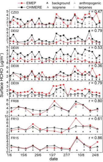
Fig. 3. Timeseries of surface HCHO concentrations during sum-mer 2003 as measured at the 8 EMEP stations and simulated by CHIMERE. The different emission contributions to the simulated surface concentrations are also given with grey symbols.
are in the range of the yields simulated by the three reference schemes. It is important to note that large uncertainties re-main in the oxidation schemes of many VOCs (e.g.α-pinene) and the error estimate deduced from the differences between the chemical schemes gives only an indication of how consis-tent the different mechanisms are and cannot be an absolute error determination.
2.3 CHIMERE evaluation with HCHO surface measure-ments
Formaldehyde simulated by CHIMERE is evaluated using surface measurements gathered within the EMEP ground-based monitoring network (http://www.nilu.no/projects/ccc/ emepdata.html). Observations are performed on a once- or twice-a-week basis. The sampling time is about 8 h centered at noon. Chemical analysis of the samples is done by re-versed phase high-performance liquid chromatography
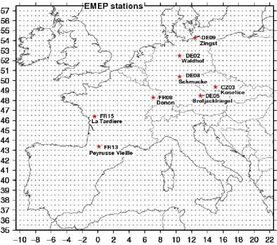
fol-lowed by UV detection (Solberg et al., 1995). The precision of the HCHO measurements has been estimated applying parallel sampling and analysis at different stations between 1995 and 2001 (Solberg et al., 1998, 2001a, b, 2005). Three consecutive years of parallel sampling at the Birkenes station (Norway) showed a measurement precision of 5–6% (Sol-berg et al., 1998). Similar analysis conducted at the French Donon station showed a precision of 7–8% in 1997 (Solberg et al., 1998) and about 13% in 1999 (Solberg et al., 2001a). However, the precision can be much smaller for some cases: an analysis between 1999 and 2001 at the German Waldhof station shows a precision of about 52% (Solberg et al., 2005). The continental version of CHIMERE has been used to simulate HCHO surface concentration over Europe during the summer 2003. The simulated surface concentrations of HCHO are interpolated at the location of the surface mea-surements at eight rural monitoring stations of the EMEP network (see Fig. 2). The station type has been character-ized using the tagged simulation results (Sect. 3), plotted in Fig. 3. The different emission contributions are of similar magnitude for the stations of Koˇsetice, Waldhof, Brotjackl-reigel, and Schm¨ucke ranging between 15 and 30%. Iso-prene oxidation is slightly the largest contribution at Brot-jacklreigel and Schm¨ucke whereas terpene oxidation is the largest at Koˇsetice. The station of Zingst, located at a remote site on the Baltic Sea coast, is largely dominated by the back-ground oxidation of methane and the stations at Donon and Peyrusse Vieille, located in remote forested areas, by the iso-prene contribution. The HCHO concentrations simulated at the La Tardi`ere station are similarly influenced by methane and isoprene oxidation.
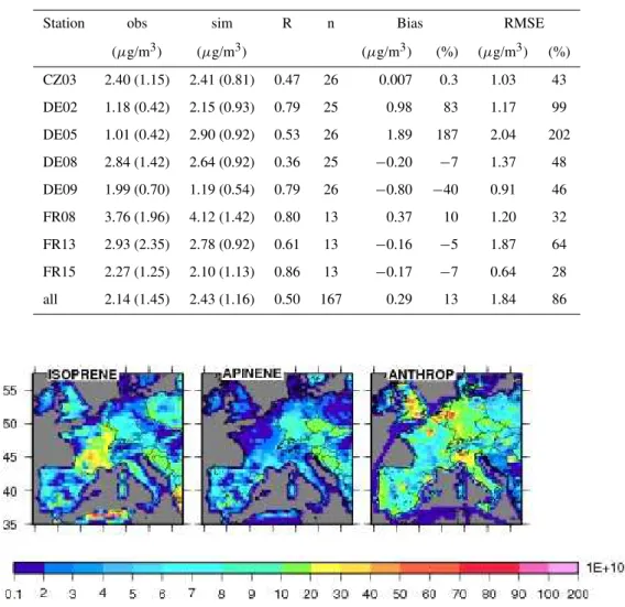
Table 3.Statistics inferred from the comparison between surface observations and simulations for the June-July-August 2003 period at each EMEP stations: obs and sim represent the mean surface concentrations of HCHO observed and simulated respectively; R is the correlation coefficient; n the number of comparison points, the bias is given as sim-obs; and RMSE is the root mean square of the error between the observations and the simulations.
Station obs sim R n Bias RMSE
(µg/m3) (µg/m3) (µg/m3) (%) (µg/m3) (%)
CZ03 2.40 (1.15) 2.41 (0.81) 0.47 26 0.007 0.3 1.03 43
DE02 1.18 (0.42) 2.15 (0.93) 0.79 25 0.98 83 1.17 99
DE05 1.01 (0.42) 2.90 (0.92) 0.53 26 1.89 187 2.04 202
DE08 2.84 (1.42) 2.64 (0.92) 0.36 25 −0.20 −7 1.37 48 DE09 1.99 (0.70) 1.19 (0.54) 0.79 26 −0.80 −40 0.91 46 FR08 3.76 (1.96) 4.12 (1.42) 0.80 13 0.37 10 1.20 32
FR13 2.93 (2.35) 2.78 (0.92) 0.61 13 −0.16 −5 1.87 64 FR15 2.27 (1.25) 2.10 (1.13) 0.86 13 −0.17 −7 0.64 28 all 2.14 (1.45) 2.43 (1.16) 0.50 167 0.29 13 1.84 86
α
Fig. 4.Mean emissions (in molecule/cm2/s) of isoprene,α-pinene, and anthropogenic VOC considered within CHIMERE for summer 2003.
from different sources are well equilibrated at these two sites, it is not obvious which process is responsible for that differ-ence. Some well admitted model errors can be cited as a potential explanation for that difference: uncertainties in dif-ferent types of VOC emissions (see below), uncertainties in the chemical scheme, uncertainties in OH concentrations af-fecting the HCHO formation and loss, uncertainties of the meteorology affecting transport patterns.
3 Contribution of the emissions to the HCHO tropo-spheric columns
The aim of the present section is to evaluate how the different types of emissions and the tropospheric columns of HCHO
Table 4.Principle of the tagging technique.
Original scheme Tagged scheme
PrimEVOC + X→SecVOCi + others PrimEVOC + X→SecVOCi∗+ PrimEVOC + X SecVOCi+ X→6SecVOCj+ others SecVOCi∗+ X→6SecVOCj∗+ X
Case when X=SecVOCj i.e. reactions of RO2+RO2type
RO2+ R
′
O2→RO + R
′
O + 2HO2 RO2∗+ R
′
O2→RO∗+ R
′ O2
RO2+ R
′
O2∗→R
′
O∗+ RO2
RO2+ R
′
O2→RO + R
′
OH RO2∗+ R
′
O2→RO∗+ R
′ O2
RO2+ R′O2∗→R′OH∗+ RO2 RO2+ R
′
O2→ROH + R
′
O RO2∗+ R
′
O2→ROH∗+ R
′ O2
RO2+ R
′
O2∗→R
′
O∗+ RO2
∗indicates tagged species
PrimEVOC=primary emitted VOC, a precursor of HCHO; SecVOC=secondary produced VOC (can be HCHO); X=OH, HO2, NO, NO2,
NO3,hν, SecVOC; others=inorganic species
α
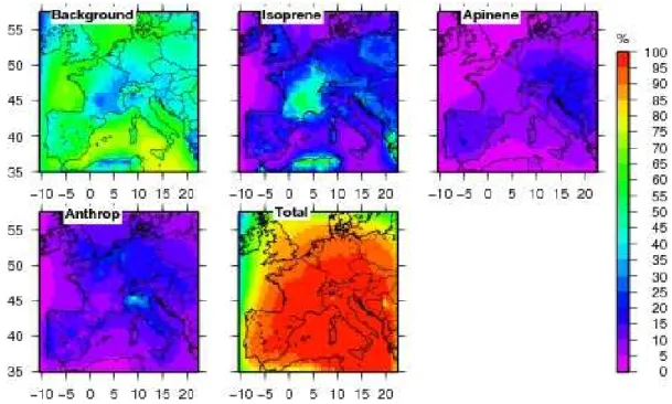
Fig. 5. Contribution (%) to the tropospheric column of HCHO from methane (background), isoprene,α-pinene, and anthropogenic VOC oxidation. The sum of the different contribution is also presented in order to provide information on the boundary condition influence (difference to 100%).
In order to identify the regions where the impact of the different emissions and their variations would be de-tectable, we included different chemical tagged schemes into the CHIMERE model. A similar technique as Pfister et al. (2008) has been used. The principle of the technique is summarized in Table 4. This technique enables the contribu-tion of different formaldehyde produccontribu-tion pathways to the tropospheric column to be tracked separately. Four
any secondary sources are considered, in order to avoid too strong complication of the tagged scheme. In particular, CH3CHO, CH3OH, and MEK are emitted but can also be
produced secondarily, and thus are not considered. This sim-plification is reasonable because the primary emissions of these 3 species are negligible compared to the other anthro-pogenic VOCs (Table 1). However, methanol has a large biogenic source that is not accounted for in CHIMERE: the biogenic part is more than one order of magnitude larger (7.4×10¹⁰molecule/cm2/s, Granier et al., 2005) than the
an-thropogenic part (0.3×10¹⁰molecule/cm2/s). To estimate the
impact of neglecting biogenic methanol on the HCHO col-umn, we calculate the total potential productions of HCHO as the sum of the individual potential production of each pre-cursor (defined as the yield of the prepre-cursor multiplied by the corresponding mean European emissions). The total po-tential production of HCHO obtained is about 10% larger when biogenic emissions of methanol are included. The rel-atively long lifetime of methanol (Table 1) suggests that the formaldehyde produced by the biogenic methanol emitted in the model domain would be widely dispersed over the do-main and would not provide any information on the emis-sions. Thus neglecting biogenic methanol introduces an er-ror on the simulated tropospheric columns of HCHO of the order of 10%.
The simulated 2003 summer means of the different con-tributions of HCHO sources are presented in Fig. 5. The re-sults are presented at 10:00 LT, i.e. at the overpass time of SCIAMACHY (see Sect. 4). The background contribution represents about 55% of the HCHO tropospheric columns on average but can be as low as a few percent in some grid cells and reaches up to 85% in some others, especially over sea. The mean isoprene contribution to the HCHO tropo-spheric column is about 17% and 21% with and without over-sea columns, respectively. Isoprene oxidation is the largest source of formaldehyde over the south-western half of France, over Greece and North Africa. It also domi-nates contributions from other emissions over Poland and the Balkans. Note that the impact of the isoprene emissions on the HCHO columns is mainly localized above the source regions. The spatial correlation (r2) between the emissions and the isoprene-tagged formaldehyde columns is 64%. This reflects the fact that isoprene is oxidized rather quickly to HCHO, i.e. largely within the same grid-cell. The terpene emissions can contribute to up to 25% of the HCHO col-umn but their mean contribution is rather low (8% on av-erage). The maxima of the contribution are also localized close to the main source regions but the spatial correlation of the tagged columns with the emissions is smaller (45%) and most likely results from the lower contribution to the HCHO columns as compared to that of isoprene. The mean contribution of the anthropogenic emissions to the HCHO column (11% on average) is also smaller compared to the isoprene contribution. The spatial correlation between the anthropogenic emissions and the tagged columns is also
re-duced (44%) compared to isoprene and only the unsaturated species significantly contribute to this correlation. Alkane emissions represented by n-butane are too unreactive to be oxidized in the same grid cell (Table 2). A large contribu-tion (up to 40%) is observed above Northern Italy with the largest columns localized above the most intense source re-gions. This implies that the influence of the most reactive species in this case like C2H4, C3H6or o-xylene (Fig. 1) on
HCHO is being observed. These molecules are also emit-ted with the same order of magnitude in the North-West of Europe but with a much smaller impact on the HCHO columns. This behavior is attributed to two factors: (i) the longer residence time of pollutants over the Po Valley (lower winds), (ii) the larger oxidative capacity of the air in this re-gion, which results from larger amounts of actinic radiation, relatively high ozone and water vapour concentrations (in-creased OH production) and lower radical losses due to lower NOx levels. Finally, the sum of all the contributions
(back-ground + emissions) is shown in Fig. 5. This map shows the influence of the boundary conditions on the HCHO tropo-spheric column (from the difference to 100%). In agreement with the dominant winds in Europe, the boundary conditions have a significant impact mainly close to the western and the northern boundary of the domain. The contribution ranges from 20 to 30% in the boundary regions to more than 70% in the extreme West of the domain. Ireland and the North of United Kingdom are the most affected areas. The contribu-tion decreases rapidly towards the interior of the domain ac-cording to the short formaldehyde lifetime of several hours.
It is also worth noting that the temporal and spatial vari-ability of the HCHO tropospheric columns is driven on av-erage over the European domain by isoprene variability, followed by the background variability. The influence of anthropogenic VOCs and terpenes is limited except in re-gions with large emissions. The temporal variability (dur-ing summertime) is estimated by the standard deviation for the mean tagged column over the European domain and then likely underestimated. The standard deviation value is 0.37×10¹⁵molecule/cm2 for isoprene-tagged columns,
0.27×10¹⁵molecule/cm2 for background-tagged columns,
and 0.10 and 0.17×10¹⁵molecule/cm2 for
the spatial variability. This suggests that if satellite data can be used to constrain emissions in Europe, isoprene emission estimates are likely the only estimates that could be con-strained. In the following, we will then concentrate on dis-cussing if satellite observations of HCHO would help to im-prove isoprene emission estimates.
4 SCIAMACHY/CHIMERE comparison over Europe in summer 2003
4.1 Data description
SCIAMACHY is an instrument operating onboard the sun-synchronous Envisat satellite since 2002 which has an equa-tor crossing time of 10:00 a.m. LT. This instrument is a spec-trometer designed to measure sunlight transmitted, reflected and scattered by the earth’s atmosphere or surface in the ul-traviolet, visible and near infrared (Bovensmann et al., 1999). The maximum scan width in the nadir-view is 960 km and global coverage is achieved within 6 days. The horizontal resolution in the nadir mode is 30×60 km2.
The retrieval of vertical columns of HCHO is based on the DOAS technique that relies on the separation of narrow band absorption signatures from broad band absorption and scattering features. The retrieval consists in the determina-tion of the slant column density of the considered species and its conversion to a vertical column amount by apply-ing an air mass factor (AMF). This accounts for the path of light through the atmosphere and takes the vertical profiles of scattering and absorbing species into account. The spec-tral region of 334–348 nm was selected for the retrieval to avoid any correlation with an instrument grating polarization structure around 360 nm. In comparison to HCHO measure-ments from GOME (Global Ozone Monitoring Experiment, e.g. Wittrock, et al., 2000) this leads to a reduced signal-to-noise-ratio. The AMF calculation uses three standard pro-files based on observations reported in literature, which are assigned to the individual pixels and times based on external information (Wittrock, 2006). Only ground scenes having less than 20 percent cloud cover are considered. Prior to con-version to vertical columns, the slant columns were normal-ized by assuming a mean value of 3.5×10¹⁵molecule.cm−2
in the region between 180◦W and 160◦W in agreement with climatological values from the MOZART (Horowitz et al., 2003) and the LMDz-INCA (Hauglustaine et al., 2004) mod-els. This normalization is necessary to compensate for offsets introduced by the solar reference measurements (Richter and Burrows, 2002) and interferences by other absorbers. The uncertainty of HCHO vertical column retrieved from SCIA-MACHY measurements depends mainly on the fitting accu-racy. For a single pixel (30×60 km2 footprint) it is about
1016molecule/cm2. By averaging both in space and time this can be significantly reduced (see section below). The sur-face spectral reflectance, the assumption for the aerosol
ver-tical distribution and its opver-tical thickness, and the assumed vertical distribution of formaldehyde in the lowermost tro-posphere contribute to the uncertainty of the AMF calcula-tion in the retrieval. This error is strongly scene-dependent but varies typically in the range of 10 to 30% of the ver-tical column. Systematic error sources are the temperature dependence of the HCHO cross section and inaccuracies of its absolute value, spectral interference in particular ozone to other trace gases and the normalization of the slant columns applying a reference sector. These sources sum up to about 3 to 5×10¹⁵molecule/cm2 depending on latitude which is
in reasonable agreement to the error budget reported in De Smedt et al. (2008). This study has also found a consistency between their and the Bremen HCHO columns within 10% above source regions. A detailed discussion of the satellite data evaluation used here can be found in Wittrock, 2006. SCIAMACHY data are regrided on a 0.5◦×0.5◦grid for an
initial use to match the model resolution. 4.2 Results
The comparison of daily SCIAMACHY observations and simulations above Europe is not reasonable be-cause the mean European column of formaldehyde (∼7×10¹⁵molecule/cm2)is smaller than the error (random error for one pixel about 1016molecule/cm2, see above). Thus, it is necessary to average the observations either tem-porally or spatially (or both) to reduce the errors. In a first step, we choose to temporally average the observations on a seasonal (summer months) and a monthly basis. The random error is reduced by the square-root of the number of SCIA-MACHY overpasses during the time period considered. On average the number of overpasses is about 6.25 per month and 18.75 per season for one pixel. A detailed calcula-tion for each pixel indicates that the total error decreases down to 3.8×10¹⁵molecule/cm2on average when
observa-tions are averaged over the 3 summer months and down to 5.4×10¹⁵molecule/cm2when the average is made over one
month. This latter error is still large compared to the mean HCHO column. In order to have comparable error level over 3 months and over one month, the observations have been regridded on a 1◦×1◦grid for the monthly means.
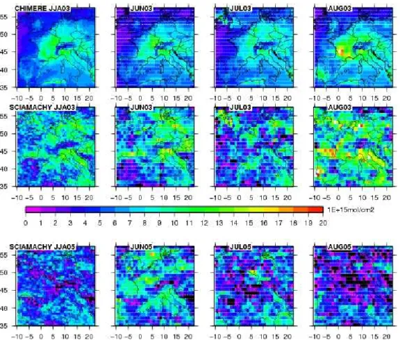
The summer and monthly tropospheric formaldehyde columns measured by SCIAMACHY in 2003 and 2005 are displayed in Fig. 6 (middle and lower panels) on a 0.5◦×0.5◦
grid for the JJA period and 1◦×1◦for individual months. For
2005 that is a rather normal year concerning climatic con-ditions the HCHO columns observed by SCIAMACHY de-crease from June to August (Fig. 6 and Table 5) but they are too close to the detection limit of the instrument to be unambiguously compared to model simulations, especially in July and August. In 2003, the mean European columns (7.33×10¹⁵molecule/cm2) for the JJA period is 50% larger
¯ ¯
Fig. 6. HCHO tropospheric columns simulated by CHIMERE in summer 2003 (top panel), observed by SCIAMACHY in summer 2003 (middle panel) and 2005 (bottom panel). Values are averaged over the 3 summer months (JJA period) and individually over each summer month. Columns are given with a 0.5◦×0.5◦resolution for the JJA period and with a 1◦×1◦resolution for the monthly mean (see text for details).
the beginning of August implied much larger biogenic emis-sions (Curci et al., 2008). Combined with stagnating anticy-clonic conditions, this leads to much larger amount of HCHO produced. The temporal evolution of HCHO columns is dif-ferent from 2005: even if the columns observed in July are smaller than those observed in June, unusually large columns are measured in August during the heat wave period (Fig. 6 and Table 5). The continental columns are generally larger than the oceanic columns in agreement with the significant part of continental emissions leading to HCHO production. The oceanic columns are quite similar between 2003 and 2005 (Table 5) except for August when heat wave influence was the largest. Moreover, the spatial variability (standard deviation) of the columns is also larger in continental areas than over ocean (Table 5). One expects that the enhanced variability is mainly due to an increased variability of the sources over land. However, some observations have to be taken with caution especially when monthly averages are considered. Their uncertainty can be in the range of their
absolute value, for instance in some regions in Spain dur-ing June and July. Some of the large columns observed over sea are also questionable because they might be artifact due to interfering contributions that can perturb the HCHO re-trieval (Wittrock, 2006). De Smedt et al. (2008) have shown that using a slightly different window for the retrieval allows avoiding some interferences and reduces the large values ob-served over sea in some but not all cases. However, large wild fires occurred in August 2003 in Portugal and Spain and consequently their emissions – not included in CHIMERE – could explain the large columns observed in the Gascony gulf (e.g. Fig. 12 in Tressol et al., 2008).
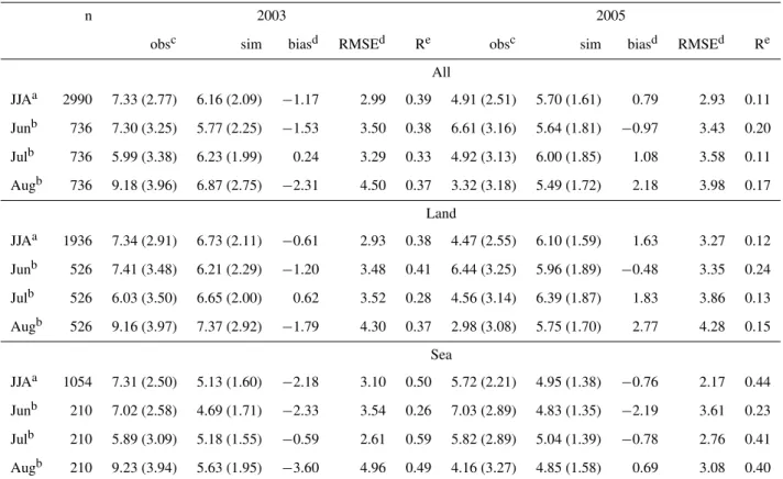
Table 5. Statistics derived from the comparison of HCHO tropospheric columns (1015molecule/cm2) observed by SCIAMACHY and simulated by CHIMERE for summer 2003 and 2005. The statistics are performed on the total domain, and on the land and sea columns, respectively.
n 2003 2005
obsc sim biasd RMSEd Re obsc sim biasd RMSEd Re
All
JJAa 2990 7.33 (2.77) 6.16 (2.09) −1.17 2.99 0.39 4.91 (2.51) 5.70 (1.61) 0.79 2.93 0.11 Junb 736 7.30 (3.25) 5.77 (2.25) −1.53 3.50 0.38 6.61 (3.16) 5.64 (1.81) −0.97 3.43 0.20 Julb 736 5.99 (3.38) 6.23 (1.99) 0.24 3.29 0.33 4.92 (3.13) 6.00 (1.85) 1.08 3.58 0.11
Augb 736 9.18 (3.96) 6.87 (2.75) −2.31 4.50 0.37 3.32 (3.18) 5.49 (1.72) 2.18 3.98 0.17 Land
JJAa 1936 7.34 (2.91) 6.73 (2.11) −0.61 2.93 0.38 4.47 (2.55) 6.10 (1.59) 1.63 3.27 0.12 Junb 526 7.41 (3.48) 6.21 (2.29) −1.20 3.48 0.41 6.44 (3.25) 5.96 (1.89) −0.48 3.35 0.24 Julb 526 6.03 (3.50) 6.65 (2.00) 0.62 3.52 0.28 4.56 (3.14) 6.39 (1.87) 1.83 3.86 0.13
Augb 526 9.16 (3.97) 7.37 (2.92) −1.79 4.30 0.37 2.98 (3.08) 5.75 (1.70) 2.77 4.28 0.15 Sea
JJAa 1054 7.31 (2.50) 5.13 (1.60) −2.18 3.10 0.50 5.72 (2.21) 4.95 (1.38) −0.76 2.17 0.44 Junb 210 7.02 (2.58) 4.69 (1.71) −2.33 3.54 0.26 7.03 (2.89) 4.83 (1.35) −2.19 3.61 0.23 Julb 210 5.89 (3.09) 5.18 (1.55) −0.59 2.61 0.59 5.82 (2.89) 5.04 (1.39) −0.78 2.76 0.41 Augb 210 9.23 (3.94) 5.63 (1.95) −3.60 4.96 0.49 4.16 (3.27) 4.85 (1.58) 0.69 3.08 0.40
aresolution 0.5◦×
0.5◦;bresolution 1◦×1◦;cThe standard deviation of the mean European HCHO columns observed by SCIAMACHY is indicated between parentheses;dThe bias and the RMSE are given in absolute value;eSpatial correlation
SCIAMACHY are qualitatively reproduced by the model (Fig. 6 – JJA period). Unusually large formaldehyde val-ues during August are also simulated by the model in agree-ment with strong heat wave conditions encountered in Eu-rope for this period. However, the magnitude of these en-hanced columns is less in the model and the spatial distribu-tion cell by cell is not well reproduced. A small tendency of the model to underestimate formaldehyde is also found for June but not for July (Table 5). The mean biases for indi-vidual months are smaller than 25% and are clearly within the measurement and model error limits. The relative RMSE (root mean square of the error) of 40–50% is large but is of the order of the SCIAMACHY uncertainties. The dif-ferences between the observations and the simulations are more important for the oceanic columns (Table 5) but these columns have to be considered with caution as mentioned previously. If one focuses on the continental part, the differ-ences are significantly reduced: the mean bias for the JJA period decreases by a factor of 2, RMSE and spatial cor-relations are rather similar. The main differences between
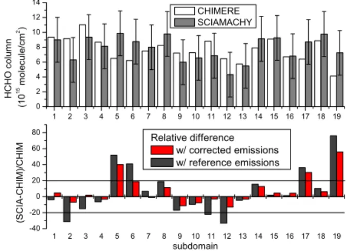
Fig. 7. Nineteen subdomains defined for SCIAMACHY and CHIMERE HCHO column comparison.
spatial correlations obtained when model and observations are compared cell by cell (Table 5) suggest that such com-parisons are not the most satisfying because significant noise remains in the measurements. Additional spatial averaging of regions with similar formaldehyde columns and type of emissions helps to reduce the measurement noise and to have more pertinent comparisons with simulations. Instead of de-grading again the horizontal resolution without any relations with the source regions, we chose to define subdomains for their consistency in terms of biogenic emissions influence onto HCHO and for the specific differences noted between SCIAMACHY and CHIMERE (e.g. South-East of France or Poland). Nineteen subdomains have been finally selected (Fig. 7). The SCIAMACHY and CHIMERE formaldehyde columns have been spatially and temporally averaged over each subdomain and compared. The total error on the SCIA-MACHY columns is now reduced to the systematic error (3×10¹⁵molecule/cm2): the random error contributes with less than 1%. The total error corresponds to 30 to 70% of the tropospheric columns depending on the subdomain.
The comparison results between SCIAMACHY and CHIMERE mean columns are shown in Fig. 8 for the JJA pe-riod. The agreement between SCIAMACHY and CHIMERE is better than 20% for the majority of the subdomains. The differences are the largest in the most northern domains (5, 6, 17, and 19), with simulated HCHO columns underesti-mated in comparison to the SCIAMACHY measurements. On the contrary, the observed columns are smaller (>20%) than the simulated ones in subdomains 2, 11 and 12. Subdo-mains 11 and 12 are also slightly impacted by the boundary conditions. Uncertainty in biogenic emissions is larger for domain 12 (North Africa) as seen previously. Thus on one hand, the differences between observations and simulations
Fig. 8.Comparison of the mean HCHO tropospheric column mea-sure by SCIAMACHY and simulated by CHIMERE in each subdo-main (upper panel). The relative differences are given in the bottom panel. The differences obtained with the corrected emission set are presented in red.
are within the SCIAMACHY errors for almost all the subdo-mains, on the other hand, they can be explained by the large uncertainties especially in biogenic emissions (see below for more detailed discussion).
5 Potential gain of satellite data use for emission esti-mates improvement
In the previous section, we defined the adequate temporal and spatial averaging needed to have reasonable uncertainties on the observations and meaningful comparisons with simula-tions. Here we use these averaged observations as constraints for biogenic emissions of isoprene, which are the strongest contributor to tropospheric HCHO columns. To this purpose, we set-up a simplified inversion scheme, i.e. we applied a Bayesian least squares method (Rodgers, 2000) to optimize the a priori source strength of biogenic isoprene in the re-duced space of the 19 subdomains defined in Sect. 4. Cor-rections of the mean emission estimates per subdomains for the summer 2003 period are inferred from the corresponding mean HCHO columns. We choose a matrix-based formula-tion for the inverse modeling as the problem to solve is of re-duced dimension. The optimized parameters are not directly the emissions of biogenic isoprene in the 19 subdomains but a vector of multiplicative control parameters, named correc-tion factor vector in the following. The a posteriori solucorrec-tion
xapand the corresponding a posteriori covariance error ma-trixPapare given by:
xap=xb+hHtR−1H+B−1i −1
HtR−1y−Hxb (1)
Pap=hHtR−1H+B−1i −1
0 1 2 3 4 5 6 7 8 9 10 11 12 13 14 15 16 17 18 19
0 1 2 3 4 5 6 7 8 9 10 11 12 13 14 15 16 17 18 19 H matrix 0.0 0.2 0.4 0.6 0.8 1.0 1.2 1.4 1.6 1.8 2.0 2.2 2.4 2.6 2.8 3.0 3.2 3.4 3.6 1E+15
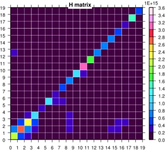
Fig. 9. Observation matrix H used for the inverse modelling exer-cise. This matrix represents the Jacobian of the model in the obser-vation space and was determined using a perturbative method (see text for details).
xbis the a priori or background correction factor vector with an unbiased Gaussian error statistics described by the covari-ance matrix B. y is the observation vector of the HCHO column with their error statistics also assumed to be unbi-ased and Gaussian, and represented by the covariance matrix
R. Note that in our case the model error statistics are in-cluded in the covariance matrixR. It is assumed that the ob-servation errors, the model errors and the background errors are respectively uncorrelated. This implies that the matrices
Rand Bare diagonal; the diagonal elements are the vari-ances of the observation squared summed with the varivari-ances of the model errors and the variances of background errors, respectively. His the observation matrix that represents the Jacobian of the model with respect to the control parame-ters (multiplicative factor of the emissions) convoluted with a projection operator mapping the model state space onto the observation space (19 subdomains). The observation matrix (H) is evaluated using a perturbative method: the emissions were increased by 20% for each subdomain separately and the sensitivity of HCHO columns was deduced for the same subdomain (diagonal terms ofH) as well as for the other subdomains (off-diagonal terms ofH). This means that 19 simulations are necessary to build theHmatrix. The results are averaged over the summer 2003 period. The off-diagonal terms of the matrix are much smaller than the diagonal terms. Indeed, the impact of one domain onto the others is always less than one third of its self-impact (Fig. 9).
The considered background errors (B) are fixed to a fac-tor of 3 according to the upper admitted uncertainties in the biogenic emissions prescribed by Simpson et al. (1999). The observation errors are close to the systematic errors
de-rived in Sect. 4.2 (about 3×10¹⁵molecule/cm2). The ob-servation error considered in the R matrix is the squared sum of this systematic part and of the random part calcu-lated for each subdomain. The model errors recalcu-lated to the chemistry scheme have been discussed in Sect. 2.3: an er-ror of 10% on the HCHO production from isoprene oxida-tion is reasonable. In addioxida-tion it is necessary to account for the terpene contribution that is largely uncertain, uncer-tainty in emissions being the major factor contributing to uncertainty. Considering the mean contribution to the col-umn (8%, Sect. 3) and an uncertainty of a factor of 3 for the emissions, the averaged error linked to terpenes can be estimated to 1.75×10¹⁵molecule/cm2 (note that again this
error is explicitly calculated for each subdomain). Com-bined with the uncertainty on the HCHO production from isoprene oxidation and the uncertainty resulting of the non-consideration of biogenic methanol, the model error amounts to 2×10¹⁵molecule/cm2on average. Note that the contribu-tion of the uncertainty on the anthropogenic part of the col-umn is negligible compared to the other error sources and thus not accounted for in the calculation of the model error.
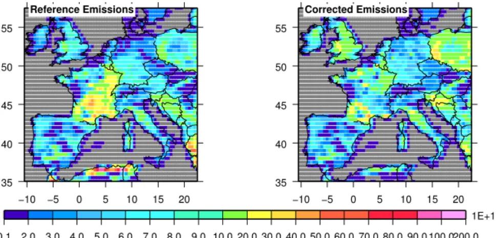
The correction factors and the a posteriori errors obtained when Eq. (1) and (2) are applied, are shown in Table 6. The new inventory of isoprene emissions obtained with the cor-rection factors is compared to the inventory used as reference in Fig. 10. The inverse modeling results suggest that iso-prene emission estimates in the eastern part of France (sub-domains 2 and 3), in Greece and North Africa (the most sen-sitive regions for isoprene emissions) should be reduced sig-nificantly. The corrections have the same sign as is obtained when comparing our reference emission inventory with the recent NATAIR inventory (Steinbrecher et al., 2009; Curci et al., 2009). A good agreement between the absolute value of the corrections obtained by this study and those suggested by the NATAIR inventory is observed for the French regions. On the contrary, emission estimates in the Northern part of Europe (subdomains 5, 6, 7, 8, 17, and 19) need to be in-creased, especially for Poland and the United Kingdom by a factor up to 2. The corrections prescribed by our method are going in the opposite direction compared to what the compar-ison between the recent NATAIR inventory and the reference inventory used here would suggest. Note also that confidence in the observations at these latitudes is reduced. Further vestigations for both the observations and the available in-ventories would be necessary to firmly conclude.
Table 6. Mean initial or a priori emissions of biogenic isoprene in each subdomain and the corrections obtained by inverse modelling (correction factor and a posteriori errors). The improvement obtained for the uncertainties on the emissions is indicated in the last column.
Domain Mean initial emissions Correction A posteriori Improvementa (1010mol/cm2/s) factor errora (%)
1 15.36 0.97 1.67 44
2 24.02 0.20 1.54 49
3 18.54 0.54 1.74 42
4 7.65 0.82 2.41 20
5 2.21 1.88 2.89 4
6 7.55 2.00 2.19 27
7 2.21 1.38 2.87 4
8 3.87 1.53 2.76 8
9 5.21 0.49 2.67 11
10 7.62 0.82 2.24 25
11 24.80 0.46 1.16 61 12 15.66 0.15 1.66 45
13 4.05 0.91 2.57 14
14 4.44 1.38 2.68 11
15 4.05 0.95 2.61 13
16 4.41 1.11 2.71 10
17 2.64 1.79 2.83 6
18 11.80 1.30 2.01 33
19 3.30 2.00 2.79 7
ato be compared to the a priori error (factor 3) considered for the biogenic isoprene emissions in this study
35 40 45 50 55
−10 −5 0 5 10 15 20
Reference Emissions
35 40 45 50 55
−10 −5 0 5 10 15 20
Corrected Emissions
0.1 2.0 3.0 4.0 5.0 6.0 7.0 8.0 9.0 10.0 20.0 30.0 40.0 50.0 60.0 70.0 80.0 90.0 100.0200.0 1E+10
Fig. 10.Comparison between the reference and the corrected biogenic isoprene emissions (in molecule/cm2/s).
In order to check the consistency of the corrections, the model was run with the inversed emission estimates. The difference between the HCHO columns from SCIAMACHY and those simulated with the new estimates are plotted in the lower panel of Fig. 8 in red. The difference is systemati-cally reduced compared to the reference case and does not exceed 20% for any of the subdomains except two of them (5 and 19).
6 Conclusions
isoprene emissions uncertainties remain. The discussion of the results required:
(1) The evaluation of the model performances and the errors (mainly related to HCHO chemistry). Comparisons with surface measurements show that the model succeeds to reproduce the basic photochemistry leading to the ob-served HCHO concentrations for most of the sites. Unfortu-nately the small number of sites operating in-situ formalde-hyde measurements does not allow a complete model evalua-tion. On the other hand, no strong inconsistencies concerning HCHO chemistry in the MELCHIOR mechanism used have been revealed. The error on the HCHO production from iso-prene oxidation is estimated to 10%. Addition of other error contributions (terpenes, methanol) leads to a model error of
∼2×10¹⁵molecule/cm2.
(2) The definition of regions of interest in Western Eu-rope for the isoprene emissions. This was achieved by implementing tagged chemical schemes in the model in order to infer the contribution of the different sources of formalde-hyde to the European tropospheric columns and then the re-gions which are most sensitive to isoprene emissions.
(3) The quantification of observation errors that also con-trolled the definition of the regions of interest stressing the needs of specific spatial and temporal averaging over coher-ent HCHO sources.
Finally, perspectives of using satellite observations as con-straint of isoprene emissions in Europe are investigated using an optimal estimation method. The inverse modeling results show that isoprene emissions in the Eastern half of France and in Greece and North Africa are overestimated in the ref-erence inventory used. In contrast, the a priori emission esti-mates seem too low in the northern part of Europe but the higher uncertainties in the observations for these latitudes does not allow a firm conclusion. In general, SCIAMACHY observations used as constraint could reduce the errors on the emission estimates more by about a factor of two in the most sensitive regions. Thus satellite formaldehyde columns are shown in this paper to give useful constraints on isoprene emissions even over Europe, where these emissions are much weaker than over North-America.
Acknowledgements. We acknowledge the authors of the datasets
of the POET inventories and the GEIA/ACCENT database activity for providing biogenic emissions of methanol. The European Centre of Medium Weather Forecast is acknowledged for use of meteorological analysis.
Edited by: P. Monks
The publication of this article is financed by CNRS-INSU.
References
Abbot, D. S., Palmer, P. I., Martin, R. V., Chance, K., Jacob, D. J., and Guenther, A.: Seasonal and interannual variability of North American isoprene emissions as determined by formaldehyde column measurements from space, Geophys. Res. Lett., 30(17), 1886, doi:10.1029/2003GL017336, 2003.
Atkinson, R.: Gas-phase tropospheric chemistry of organic com-pounds, J. Phys. Chem. Ref. Data Monogr., 2, 13–46, 1994. Aumont, B., Szopa, S., and Madronich, S.: Modelling the evolution
of organic carbon during its gas-phase tropospheric oxidation: development of an explicit model based on a self generating ap-proach, Atmos. Chem. Phys., 5, 2497–2517, 2005,
http://www.atmos-chem-phys.net/5/2497/2005/.
Beekmann, M. and Derognat, C.: Monte Carlo uncertainty anal-ysis of a regional-scale transport chemistry model constrained by measurements from the Atmospheric Pollution Over the Paris Area (ESQUIF) campaign, J. Geophys. Res., 108(D17), 8559, doi:10.1029/2003JD003391, 2003.
Bessagnet, B., Hodzic, A., Vautard, R., Beekmann, M., Cheinet, S., Honor, C., Liousse, C., and Rouil, L.: Aerosol modeling with CHIMERE – Preliminary evaluation at the continentale scale, Atmos. Environ., 38, 2803–2817, 2004.
Blond, N., Bel., L., and Vautard, R.: Three-dimensional ozone dara analysis with an air quality model over the Paris area, J. Geophys. Res., 108(D23), 4744, doi:10.1029/2003JD003679, 2003. Blond, N. and Vautard, N.: Three-dimensional ozone analyses and
their use for short-term ozone forecasts, J. Geophys. Res., 109, D17303, doi:10.1029/2004JD004515, 2004.
Blond, N., Boersma, K. F., Eskes, H. J., van der A, R. J., Van Roozendeal, M., De Smedt, I., Bergametti, G., and Vautard, R.: Intercomparison of SCIAMACHY nitrogen dioxide ob-servations, in situ measurements and air quality modeling re-sults over Western Europe, J. Geophys. Res., 112, D10311, doi:10.1029/2006JD007277, 2007.
Boissard, C., Chervier, F., and Dutot, A. L.: Assessment of high (diurnal) to low (seasonal) frequency variations of isoprene emis-sion rates using a neural network approach, Atmos. Chem. Phys., 8, 2089–2101, 2008,
http://www.atmos-chem-phys.net/8/2089/2008/.
Bovensmann, H., Burrows, J. P., Buchwitz, M., Frerick, J., No¨el, S., Rozanov, V., Chance, K., and Goede, A. H. P.: SCIAMACHY: mission objectives and measurement modes, J. Atmos. Sci., 56, 127–150, 1999.
Carter, W. P. L.: Documentation of the SAPRC-99 chemical mecha-nism for the VOC reactivity assessment, Final Report to the Cali-fornia Air Resources Board under Contracts 92-329 and 95-308, Center of Environmental Research and Technology, Riverside, http://www.engr.ucr.edu/∼carter/absts.htm#saprc99, 2000.
Camredon, M., Aumont, B., Lee-Taylor, J., and Madronich, S.: The SOA/VOC/NOxsystem: an explicit model of secondary organic
aerosol formation, Atmos. Chem. Phys., 7, 5599–5610, 2007, http://www.atmos-chem-phys.net/7/5599/2007/.
Chance, K., Palmer, P. I., Spurr, R. J. D., Martin, R. V., Kurosu, T. P., and Jacob, D.: Satellite observations of formaldehyde over North America from GOME, Geophys. Res. Lett., 27, 3461– 3464, 2000.
levels, Atmos. Environ., 43, 1444–1455, 2009.
Deguillaume, L., Beekmann, M., and Menut, L.: Bayesian Monte Carlo analysis applied to regional-scale inverse emission mod-eling for reactive trace gases, J. Geophys. Res., 112, D02307, doi:10.1029/2006JD007518, 2007.
De Smedt, I., M¨uller, J.-F., Stavrakou, T., van der A, R., Eskes, H., and Van Roozendael, M.: Twelve years of global observations of formaldehyde in the troposphere using GOME and SCIA-MACHY sensors, Atmos. Chem. Phys., 8, 4947–4963, 2008, http://www.atmos-chem-phys.net/8/4947/2008/.
Friedrich, R.: GENEMIS: Assessment, improvement, temporal and spatial disaggregation of European emission data, in: Tropo-spheric Modelling and Emission Estimation, part 2, edited by: Ebel, A., Friedrich, R., and Rhode, H., 181–214, Springer, New-York, 1997.
Fu, T., Jacob, D. J., Palmer, P. I., Chance, K., Wang, Y. X., Barletta, B., Blake, D. R., Stanton, J. C., and Pilling, M. J.: Space-based formaldehyde measurements as constraints on volatile organic compound emissions is east and south Asia and implications for ozone, J. Geophys. Res., 112, D06312, doi:10.1029/2006JD007853, 2007.
Guenther, A., Hewitt, C. N., Erickson, D., Fall, R., Geron, C., Graedel, T., Harley, P., Klinger, L., Lerdau, M., McKay, W. A., Pierce, T., Scholes, B., Steinbrecher, R., Tallamraju, R., Taylor, J., and Zimmerman, P.: A global model of natural volatile or-ganic compound emissions, J. Geophys. Res., 100, 8873–8892, 1995.
Guenther, A., Karl, T., Harley, P., Wiedinmyer, C., Palmer, P. I., and Geron, C.: Estimates of global terrestrial isoprene emissions using MEGAN (Model of Emissions of Gases and Aerosols from Nature), Atmos. Chem. Phys., 6, 3181–3210, 2006,
http://www.atmos-chem-phys.net/6/3181/2006/.
Granier, C., Lamarque, J. F., Mieville, A., Muller, J. F., Olivier, J., Orlando, J., Peters, J., Petron, G., Tyndall, G., and Wal-lens, S.: POET, a database of surface emissions of ozone pre-cursors, available on internet at http://www.aero.jussieu.fr/projet/ ACCENT/POET.php, 2005.
Hauglustaine, D. A., Hourdin, F., Jourdain, L., Filiberti, M.-A., Walters, S., Lamarque, J.-F., and Holland, E. A.: Interac-tive chemistry in the Laboratoire de M´et´eorologie Dynamique general circulation model: Description and background tropo-spheric chemistry evaluation, J. Geophys. Res., 109, D04314, doi:10.1029/2003JD003957, 2004.
Honor´e C., Rou¨ıl, L., Vautard, R., Beekmann, M., Bessagnet, B., Dufour, A., Elichegaray, C., Flaud, J.-M., Malherbe, L., Meleux, F., Menut, L., Martin, D., Peuch, A., Peuch, V. H., and Poisson, N.: Predictability of European air quality: The assessment of three years of operational forecasts and analyses by the PREV’AIR system, J. Geophys. Res., D113, D04301, doi:10.1029/2007JD008761, 2008.
Horowitz, L. W., Walters, S., Mauzerall, D. L., et al.: A global simu-lation of tropospheric ozone and related tracers: Description and evaluation of MOZART, version 2, J. Geophys. Res., 108(D24), 4784, doi:10.1029/2002JD002853, 2003.
Jenkin, M. E., Saunders, S. M., Wagner, V., and Pilling, M. J.: Pro-tocol for the development of the Master Chemical Mechanism, MCM v3 (Part B): tropospheric degradation of aromatic volatile organic compounds, Atmos. Chem. Phys., 3, 181–193, 2003, http://www.atmos-chem-phys.net/3/181/2003/.
Konovalov, I. B., Beekmann, M., Richter, A., and Burrows, J. P.: Inverse modelling of the spatial distribution of NOxemissions
on a continental scale using satellite data, Atmos. Chem. Phys., 6, 1747–1770, 2006,
http://www.atmos-chem-phys.net/6/1747/2006/.
Konovalov, I. B., Beekmann, M., Burrows, J. P., and Richter, A.: Satellite measurement based estimates of decadal changes in Eu-ropean nitrogen oxides emissions, Atmos. Chem. Phys., 8, 2623– 2641, 2008, http://www.atmos-chem-phys.net/8/2623/2008/. Lathi`ere, J., Hauglustaine, D. A., Friend, A. D., De
Noblet-Ducoudr´e, N., Viovy, N., and Folberth, G. A.: Impact of climate variability and land use changes on global biogenic volatile or-ganic compound emissions, Atmos. Chem. Phys., 6, 2129–2146, 2006, http://www.atmos-chem-phys.net/6/2129/2006/.
Lattuati, M.: Contribution `a l’´etude du bilan de l’ozone tro-posph´erique `a l’interface de l’Europe et de l’Atlantique Nord: Mod´elisation lagrangienne et mesures en altitude, PhD thesis, Universit´e Paris 6, Paris, 1997.
Mandrovich, S. and Flocke, S.: The role of solar radiation in atmo-spheric chemistry, in: Handbook of Environmental Chemistry, edited by: Boule, P., Springer, New York, 1–26, 1998.
Menut, L., Vautard, R., Flamant, C., Abonnel, C., Beekmann, M., Chazette, P., Flamant, P. H., Gombert, D., Gu´edalia, D., Kley, D., Lefebvre, M. P., Lossec, B., Martin, D., M´egie, G., Perros, P., Sicard, M., and Toupance, G.: Measurements and modelling of atmospheric pollution over the Paris area: An overview of the ESQUIF project, Ann. Geophys., 18, 1467–1481, 2000, http://www.ann-geophys.net/18/1467/2000/.
Menut, L.: Adjoint modelling for atmospheric pollution process sensitivity at regional scale, J. Geophys. Res., 108(D17), 8562, doi:10.1029/2002JD002549, 2003.
Meyer-Arnek, J., Ladst¨atter-Weißenmayer, Richter, A., Wittrock, F., and Buurows, J. P.: A study of the trace gas columns of O3, NO2, and HCHO over Africa in September 1997, Faraday
Dis-cuss., 130, 387–405, 2005.
Middleton, P., Stockwell, W. R., and Carter, W. P.: Aggregation and analysis of volatile organic compound emissions for regional modelling, Atmos. Environ., 24, 1107–1133, 1990.
Millet, D. B., Jacob, D. J., Boersma, K. F., Fu, T., Kurosu, T. P., Chance, K., Heald, C. L., and Guenther, A.: Spatial distribu-tion of isoprene emissions from North America derived from formaldehyde column measurements by the OMI satellite sen-sor, J. Geophys. Res., 113, D02307, doi:10.1029/2007JD008950, 2008.
M¨uller, J.-F., Stavrakou, T., Wallens, S., De Smedt, I., Van Roozen-dael, M., Potosnak, M. J., Rinne, J., Munger, B., Goldstein, A., and Guenther, A. B.: Global isoprene emissions estimated using MEGAN, ECMWF analyses and a detailed canopy environment model, Atmos. Chem. Phys., 8, 1329–1341, 2008,
http://www.atmos-chem-phys.net/8/1329/2008/.
Palmer, P. I., Jacob, D. J., Chance, K., Martin, R. V., Spurr, R. J. D., Kurosu, T. P., Bey, I., Yantosca, R., Fiore, A., and Li, Q.: Air mass factor formulation for spectroscopic measurements from satellites: Application to formaldehyde retrievals from the Global Ozone Monitoring Experiment, J. Geophys. Res., 106(D13), 14539–14550, 2001.
J. Geophys. Res., 108(D6), 4180, doi:10.1029/2002JD002153, 2003.
Palmer, P. I., Abbot, D. S., Fu, T., Jacob, D. J., Chance, K., Kurosu, T. P., Guenther, A., Wiedinmyer, C., Stanton, J. C., Pilling, M. J., Pressley, S. N., Lamb, B., and Sumner, A. L.: Quantifying the seasonal and interannual variability of North American isoprene emissions using satellite observations of the formaldehyde column, J. Geophys. Res., 11, D12315, doi:10.1029/2005JD006689, 2006.
Pfister, G. G., Emmons, L. K., Hess, P. G., Lamarque, J.-F., Orlando, J. J., Walters, S., Guenther, A., Palmer, P. I., and Lawrence, P. J.: Contribution of isoprene to chemical budgets: A model tracer study with the NCAR CTM MOZART-4, J. Geo-phys. Res., 113, D05308, doi:10.1029/2007JD008948, 2008. Pison, I., Menut, L., and Bergametti, G.: Inverse modeling of
sur-face NOxanthropogenic emission fluxes in the Paris area during
the air pollution over Paris Region (ESQUIF) campaign, J. Geo-phys. Res., 112, D24302, doi:10.1029/2007JD008871, 2007. Richter, A. and Burrows, J. P.: Tropospheric NO2 from GOME
measurements, Adv. Space Res., 29, 1673–1683, 2002. Rodgers, C. D.: Inverse Methods for Atmospheric Sounding:
The-ory and Practice, World Sci., Hackensack, N.J, 2000.
Saunders, S. M., Jenkin, M. E., Derwent, R. G., and Pilling, M. J.: Protocol for the development of the Master Chemical Mechanism, MCM v3 (Part A): tropospheric degradation of non-aromatic volatile organic compounds, Atmos. Chem. Phys., 3, 161–180, 2003,
http://www.atmos-chem-phys.net/3/161/2003/.
Schmidt, H., Derognat, C., Vautard, R., and Beekmann, M.: A com-parison of simulated and observed ozone mixing ratios for sum-mer of 1998 in western Europe, Atmos. Environ., 35, 6277–6297, 2001.
Shim, C., Wang, Y., Choi, Y., Palmer, P. I., Abbot, D. S., and Chance, K.: Constraining global isoprene emissions with Global Ozone Monitoring Experiment (GOME) formalde-hyde column measurements, J. Geophys. Res., 110, D24301, doi:10.1029/2004JD005629, 2005.
Simpson, D., Winiwater, W., Borjesson, G., Cinderby, S., Ferreiro, A., Guenther, A., Hewitt, C. N., Janson, R., Khalil, M. A. K., Oen, S., Svennson, B. H., Tarrason, L., and Oquist, M. G., J. Geophys. Res., 104, 8113–8152, 1999.
Solberg, S., Dye, C., Scmidbauer, N., and Simpson, D.: Eval-uation of the VOC measurement programme within EMEP, NILU:EMEP/CCC-Report 5/95, ref. O-8852, June 1995. Solberg, S., Coddeville, P., Dye, C., Honz`ak, J., and Scmidbauer,
N.: VOC measurements 1997, NILU:EMEP/CCC-Report 4/08, ref. O-92016, August 1998.
Solberg, S., Dye, C., Roemer, M., and Schmidbauer, N.: VOC measurements 1999, NILU:EMEP/CCC-Report 7/2001, ref. O-92016, July 2001, 2001a.
Solberg, S., Dye, C., Walker, S. E., and Simpson, D.: Long-term measurements and model calculations of formaldehyde at ru-ral European monitoring sites, Atmos. Environ., 35, 195–207, 2001b.
Solberg, S.: VOC measurememts 2003, NILU:EMEP/CCC-Report 10/2005, ref. O-92016, August 2005.
Stavrakou, T., M¨uller, J.-F., De Smedt, I., Van Roozendael, M., van der Werf, G. R., Giglio, L., and Guenther, A.: Evaluating the performance of pyrogenic and biogenic emission inventories against one decade of space-based formaldehyde columns, At-mos. Chem. Phys., 9, 1037–1060, 2009,
http://www.atmos-chem-phys.net/9/1037/2009/.
Stohl, A., Williams, E., Wotawa, G., and Kromp-Kolb, H.: A Eu-ropean inventory of soil nitric oxide emissions and the effect of these emissions on the photochemical formation of ozone, At-mos. Environ., 30, 3741–3755, 1996.
Steinbrecher, R, Smiatek, G., K¨oble, R, Seufert, G., Theloke, J., Hauff, K., Ciccioli, P., Vautard, R., and Curci, G. : Intra- and inter-annual variability of VOC emissions from natural and semi-natural vegetation in Europe and neighbouring countries, Atmos. Environ., 43, 1380–1391, 2009.
Tiedtke, M.: A comprehensive mass flux scheme for cumulus parametrization in large-scale models, Mon. Weather Rev., 117, 1779–1800, 1989.
Tressol, M., Ordonez, C., Zbinden, R., Brioude, J., Thouret, V., Mari, C., Nedelec, P., Cammas, J.-P., Smit, H., Patz, H.-W., and Volz-Thomas, A.: Air pollution during the 2003 European heat wave as seen by MOZAIC airliners, Atmos. Chem. Phys., 8, 2133–2150, 2008,
http://www.atmos-chem-phys.net/8/2133/2008/.
Vautard, R., Beekmann, M., Roux, J., and Gombert, D.: Validation of a hybrid forecasting system for the ozone concentrations over the Paris area, Atmos. Environ., 35, 2449–2461, 2001.
Vautard, R., Martin, D., Beekmann, M., et al.: Paris emission in-ventory diagnostics from ESQUIF airborne measurements and a chemistry transport model, J. Geophys. Res., 108(D17), 8564, doi:10.1029/2002JD002797, 2003.
Vautard, R., Szopa, S., Beekmann, M., Menut, L., Hauglus-taine, D. A., Rouil, L., and Roemer, M.: Are decadal an-thropogenic emission reductions in Europe consistent with sur-face ozone observations?, Geophys. Res. Lett., 33, L13810, doi:10.1029/2006GL26080, 2006.
Vestreng, V., Adams, M., and Goodwin, J.: Inventory review 2004, Emission Data reported to CLRTAP and under the NEC Di-rective, EMEP/EEA Joint Review Report, EMEP/MSC-W Note 1/2004, ISSN 0804-2446, 2004.
Wittrock, F.: The retrieval of oxygenated volatile organic com-pounds by remote sensing techniques. Institute of Environ-mental Physics. Bremen: University of Bremen, 192, http:// nbn-resolving.de/urn:nbn:de:gbv:46-diss000104818, 2006. Wittrock, F., Richter, A., Ladst¨atter-Weißenmayer, A., and
Bur-rows, J. P.: Global Observations of Formaldehyde, ERS-ENVISAT symposium, ESA, Gothenburg, http://earth.esa.int/ pub/ESA DOC/gothenburg/238wittr.pdf., 2000.