Thermoinduced plastic flow and shape memory
effects
Heng Xiao∗ Otto T.Bruhns† Albert Th.M.Meyers‡
Abstract
We propose an enhanced form of thermocoupled J2-flow models of finite deformation elastoplasticity with temperature-dependent yielding and hard-ening behaviour. The thermomechanical constitutive structure of these models is rendered free and explicit in the rigorous sense of thermody-namic consistency. Namely, with a free energy function explicitly intro-duced in terms of almost any given form of the thermomechanical consti-tutive functions, the requirements from the second law are identically ful-filled with positive internal dissipation. We study the case when a depen-dence of yielding and hardening on temperature is given and demonstrate that thermosensitive yielding with anisotropic hardening may give rise to appreciable plastic flow either in a process of heating or in a cyclic process of heating/cooling, thus leading tothe findings of one- and two-way ther-moinduced plastic flow. We then show that such theoretical findings turn out to be the effects found in shape memory materials, such as one- and two-way memory effects. Thus, shape memory effects may be explained to be thermoinduced plastic flow resulting from thermosensitive yielding and hardening behaviour. These and other relevant facts may suggest that, from a phenomenological standpoint, thermocoupled elastoplastic J2-flow models with thermosensitive yielding and hardening may furnish natural, straightforward descriptions of thermomechanical behaviour of shape memory materials.
Keywords: thermomechanics, plasticity, shape memory, two-way mem-ory.
∗Lehrstuhl f¨ur Kontinuumsmechanik, Ruhr-Universit¨at Bochum, Germany, e-mail:
†Lehrstuhl f¨ur Mechanik – Kontinuumsmechanik, Institut f¨ur Computational Engineering,
Ruhr-Universit¨at Bochum,D-44780 Bochum, Germany, e-mail: [email protected]
‡Lehrstuhl f¨ur Mechanik – Kontinuumsmechanik, Institut f¨ur Computational Engineering,
Ruhr-Universit¨at Bochum, D-44780 Bochum, Germany, e-mail: [email protected]
1
Introduction
It is well-known that, with moderate temperature changes, usual elastoplastic materials undergo merely small recoverable thermal deformations. It may be noticeable that appreciable plastic flows may be induced during a process of pure temperature change. This may be exemplified with a metal bar displaying appreciable lengthening or shortening effects at heating or cooling.
The main objective of this article is to show that thermocoupled finite strain elastoplasticJ2-flow models with thermosensitive yielding and hardening
behaviour may indeed exhibit the noticeable effect mentioned above. Towards this objective, specific models with non-linear combined hardening should be established in a rigorous sense of thermodynamic consistency. This might be a formidable task in a broad sense without ad hoc assumptions or limitations. In a latest development by Xiao et al. [1], a free, explicit formulation of thermocoupled finite elastoplasticity with non-linear combined hardening is proposed in a rigorous sense of thermodynamic consistency. It is demon-strated that such formulation identically fulfils the second law and leads to positive internal dissipation for any given form of the thermomechanical con-stitutive functions introduced, such as yield function and non-linear hardening functions.
In the subsequent development, we shall use thermocoupled finite strainJ2
-flow models based on the aforementioned free, explicit formulation. With such models, we shall study thermosensitive yielding and hardening behaviour, and demonstrate that thermosensitive yielding with anisotropic hardening may give rise to appreciable plastic flow in a process of pure temperature change. This leads to the finding ofthermoinduced plastic flow resulting from thermosensitive yielding and hardening behaviour. Then we shall show that such theoretical findings may become noticeable with the fact that they may be explained to be the shape memory effects found in these materials. Indeed, we shall indicate that, from a phenomenological standpoint, the aforementioned findings may furnish natural, straightforward descriptions and explanations of remarkable one- and two-way memory effects observed in shape memory materials (see, e.g., [2–4]).
The main content of this article will be organised as follows. In Section 2 we introduce an enhanced form of thermocoupled finite elastoplasticJ2-flow
explaining the one-way effect from a straightforward phenomenological view-point. In Section 4 we further show that appreciable two-way plastic flow may be induced in a cyclic process of heating/cooling with constant stress. In Sec-tion 5, we demonstrate that these findings of thermoinduced plastic flows turn out to explain one- and two-way memory effects found in shape memory materi-als, from a phenomenological viewpoint. Simple forms of constitutive functions are presented as illustrative examples in Section 6, and a direct scheme for the determination of the constitutive parameters is proposed in Section 7. Finally, we discuss the main ideas and results in Section 8.
To conclude this introduction, we shortly explain notations that will fre-quently be used. A superposed dot means the material time derivative. The 2nd-order identity tensor is denoted I. Moreover, let S and T be 2nd-order tensors. Then S :T is the double dot product (scalar product) of S and T, i.e. in a Cartesian coordinate system
S:T =SijTij.
In particular, the trace of tensor S is given by S :I and denoted trS. More-over, |S|is used to designate the magnitude of tensor S:
trS =S :I =Sii, |S|= √
S :S= √
tr (S ST).
The normalisation of non-vanishing tensor S is denoted [S] and given by
[S] = S
|S|.
2
Enhanced form of thermocoupled finite strain
J
2-flow models
Classical J2-flow models for small deformation behaviour of elastoplastic
In a broad case with coupled thermal effects, general forms of thermome-chanical constitutive relations of finite elastoplasticity should be placed on uni-versal thermodynamic foundations centred on the internal dissipation and the irreversibility property of macroscopic material behaviour. Without ad hoc as-sumptions or simplifications, this might be a formidable task. Usually, implicit results are presented in conjunction with certain restrictions derived from the thermodynamic laws. Studies on thermodynamic foundations of elastoplastic formulations were made for small deformation case earlier by, e.g., [12–16] and recently by, e.g., [17–19], and for finite deformation case by [20–39].
A consistent, explicit Eulerian formulation of thermocoupled finite elasto-plasticity is established in [1]. As mentioned earlier, this recent formulation automatically fulfils the second law with general free forms of thermomechan-ical constitutive functions introduced. In what follows we shall propose an enhanced form of thermocoupled finite strainJ2-flow models based on the new
explicit formulation.
Consider a material body undergoing a process of finite deformations. Let X andxbe the position vectors of a material point in an initial and a current configuration of this body, respectively. Then, the local deformation state of this body is described by the deformation gradientF and the changing rate of the deformation state is characterised by the velocity gradientL
F = ∂x
∂X, L=
∂x˙
∂x = ˙F F −1.
The symmetric and antisymmetric parts of the latter yield the stretching (resp. natural deformation rate, Eulerian strain rate, etc.) Dand the vorticity tensor W
D= 1
2(L+L
T), W = 1
2(L−L
T).
Letσ be the Cauchy stress. Then the Kirchhoff stress is
τ =Jσ
withJ = detF the volumetric ratio (Jacobian).
In [40] self-consistent Eulerian J2-flow models of finite deformation
2.1 Eulerian thermocoupled elastoplasticity with combined hard-ening
For a current elastoplastic deformation state, the stretching D is assumed to be decomposed into two parts
D=De+Dp. (1)
In the above, the thermoelastic partDeis related to thermoelastic behaviour, while the plastic partDpis responsible for plastic flow. Consistent constitutive characterisations for them should be presented, as will be shown below.
An objective Eulerian rate equation of Hookean type is used to relate the thermoelastic partDeand an objective stress rateτoas well as the temperature rate ˙T:
De= 1 2G
o
τ− ν
E
(
trτo)I+βT˙I. (2)
Here,G,ν,E,β are the shear modulus, Poisson’s ratio, Young’s modulus and thermal expansion coefficient.
Prior to the yielding (hence De=D), the elastic rate equation (2) should be exactly integrable to deliver a hyperelastic stress-strain relation based on an elastic stored-energy function. As demonstrated in [40–44], the just-mentioned requirement is fulfilled if and only if the stress rateτo in (2) is the corotational logarithmic rate as defined below (see, e.g., [45–47]):
o
τ = ˙τ+τΩ−Ωτ, (3)
with the logarithmic spin:
Ω=W + m ∑
r=1
m ∑
s=1, s̸=r (
1 + (br/bs) 1−(br/bs)
+ 2
ln(br/bs) )
BrD Bs, (4)
where bt and Bt are the m distinct eigenvalues and the corresponding eigen-projections of the Cauchy-Green tensorB =F FT, respectively.
As shown in [48] in isothermal case, a weakened form of Ilyushin postulate implies that the plastic partDp should be governed by the normality rule. For a general case with thermal effect, this leads to the following flow rule [1]:
Dp =ξ fˆ h
∂f
In the above,f is the yield function and ˆf is given by
ˆ f = ∂f
∂τ :
o
τ+ ∂f
∂T T .˙ (6)
handξin eq. (5), known as plastic indicator and plastic modulus, will be given slightly later.
To characterise the hardening behaviour, namely the changing of the yield surface with the development of plastic flow, we introduce two hardening vari-ables. One is the plastic workκ, as defined by the following rate equation:
˙
κ=τ :Dp. (7)
This variable will enter the yield function and characterise isotropic harden-ing behaviour. The other hardenharden-ing variable is known as back stress tensor. It was introduced originally by Prager [49] and intended for describing anisotropic or kinematic hardening, as exemplified by Bauschinger effects in uniaxial de-formations of bars. In an idealised sense, such hardening effect is related to translation of the initial yield surface in stress space. The back stress α is determined by the following evolution equation:
o
α=cDp. (8)
The variablecin the above may be referred to as Prager’s hardening modulus, or simply Prager’s modulus. Initially, it was taken to be constant with the dimension of stress. This case is known as linear anisotropic hardening. Later on, Prager’s modulus c was taken to be dependent on the hardening variable κ; refer to, e.g., [7, 50–52]. In a general case with thermal effects, it may rely on bothκ and temperatureT. Then, we have
c=c(κ, T). (9)
It is demonstrated in [43] that the rateαo in eq. (8) should also be the corota-tional logarithmic rate, namely,
o
α= ˙α+αΩ−Ωα
2.2 Thermocoupled J2-flow models with thermoinducer
With the two hardening variables κ and α, the yield function f in a general sense is of the form
f =f(τ,α, κ).
In the subsequent development, this function is taken to be an enhanced form
of von Mises yield function below:
f = 1
2 |ϱτ˜−α|
2
−13r2, (10)
where ˜τ is the deviatoric stress, i.e.
˜
τ =τ −1
3(trτ)I
and r is known as the current yield stress. Isotropic hardening behaviour means that the current yield stress r should rely on the plastic work κ (see, e.g. [10, 53, 54]). Generally, it depends on both κ andT
r =r(κ, T). (11)
Moreover, the scalar factor ϱ in eq. (10) is a non-dimensional temperature-dependent positive constitutive quantity, viz.
ϱ=ϱ(T)>0. (12)
The introduction of the factor ϱ, referred to as thermoinducer, is intended for enhancing and extending the classical yield function of von Mises type by allowing for coupling effects of temperature on yielding. For the isothermal case, ϱ is a constant, and then eq. (10) reduces to the classical case. For the non-isothermal case, taking a constantϱ also leads to the classical case.
yielding is then induced in a following process of reverse, compressive load. On the other hand, in the case of pure temperature change, by analogy we may infer that plastic flow may first be induced at a process of heating and reverse plastic flow at a following process of cooling. Such two-way thermoinduced plastic flows would not be possible, according to classical form of von Mises yield function with a temperature-dependent yield stress r, since therein the effective stress |τ˜−α| keeps unchanged with constant τ and α at a process of pure temperature change. Thus, it follows that reverse plastic flow would not be induced in any process of cooling, since the yield condition could not be fulfilled.
An idea to bypass the above situation is to find out a certain means by which temperature change may be parallel to load change and then contribute to the effective stress. This idea leads to the introduction of the thermoinducer ϱ=ϱ(T) and then to the enhanced form of von Mises yield function with the combined effective stress |ϱ(T) ˜τ −α|. Now the direct coupling of the current temperatureT on the current stress level becomes clear. Also, it may be clear that temperature change indeed becomes parallel to load (stress) change. Here it may be essential that the geometrical meaning of both the yield stress as the radius of the current yield surface (work hardening) and the back stressα as the center of the current yield surface (induced anisotropy) are kept intact as in the classical von Mises yield function, while the current temperature T and the current deviatoric stress ˜τ are combined in a parallel sense to yield a new, combined effective stress, namely, |ϱ(T) ˜τ −α|. On account of this, the latter may be referred to as thermocoupled effective stress. Then, according to the enhanced form of von Mises yield function, the yielding behaviour in a thermocoupled case is characterised by the thermocoupled effective stress with the thermoinducer ϱ, in conjunction with a temperature-dependent current yield stress r. Note that both ϱ and r are constitutive functions representing thermocoupled yielding behaviour.
It will be seen in Sections 4 and 5 that the factor ϱ will be essential for the findings of two-way thermoinduced plastic flows in a cyclic heating/cooling process.
With an enhanced form of the von Mises yield function given by eq. (10), we have the following derivatives
∂f
∂τ =ϱ(ϱτ˜−α),
∂f
∂α =−(ϱτ˜−α),
∂f ∂κ =−
2 3r
∂r ∂T,
∂f ∂T =−
2 3r
∂r ∂T +ϱ
From the first in the above and the normality rule (5), we obtain
Dp =ξ ϱfˆ
h(ϱτ˜−α). (13)
Here and henceforth, the derivative of each function of temperature,ϕ=ϕ(T), is designated byϕ′, namely,
ϕ′ = dϕ dT.
Now we specify the plastic indicator ξ and the plastic modulus h. The latter is determined by the consistency condition for plastic flow
h=−∂f ∂κ
( τ : ∂f
∂τ )
−c∂f ∂τ :
∂f ∂α
for a yield function f = f(τ,α, κ) in general form. For a von Mises yield function as given by eq. (10), using the above results for the derivatives, we deduce
h= 2 3ϱ c r
2+2
3ϱ r ∂r
∂κ(ϱτ˜−α) :τ. (14) The plastic indicator ξ is associated with the loading-unloading conditions. It takes values 1 and 0 for loading and for unloading, respectively. Unified loading-unloading conditions for both strain-hardening (h > 0) and strain-softening (h <0) materials are proposed in [1]. Following these conditions, we have
ξ =
1 if f = 0, fˆ h ≥0,
0 if f <0 or (f = 0, f <ˆ 0).
(15)
In the above, the plastic modulus h is given by eq. (14), and the ˆf is of the form:
ˆ
f =ϱ(ϱτ˜−α) :τo+ (
ϱ′(ϱτ˜−α) :τ −2 3r
∂r ∂T
) ˙
T . (16)
Eqs. (1)–(16) establish thermocoupledJ2-flow models of finite
A complete coupled thermomechanical system governing the fields of deforma-tion, stress and temperature are presented by the foregoing thermomechanical constitutive equations, in conjunction with a heat conduction equation and an energy equilibrium equation in explicit form. Details are no longer given here and may be found in [1].
2.3 Thermodynamic consistency in free and explicit sense Studies of elastoplastic behaviour and its models rarely make reference to ther-modynamic requirements. It may not be clear whether the restrictions from thermodynamics would be fulfilled or not. As is usually known, a thermo-coupled theory is not “free” and “explicit”, in the sense that the constitutive functions involved as well as the thermomechanical process should be restricted by universal thermodynamic laws. Since the free energy and the entropy as central physical quantities are coupled with each other and may be elusive in concept, usually without additional assumptions and simplifications a consti-tutive formulation could not be freed from the second law formulated by the Clausius-Duhem inequality. That may be the case especially for thermocoupled elastoplasticity at finite deformations. In [1], for an Eulerian thermocoupled elastoplastic formulation of general form, a free energy function and then an entropy function are found in explicit form, which automatically fulfil the sec-ond law with positive intrinsic dissipation for any given forms of constitutive functions introduced.
Here, by applying the general result in the foregoing development, the enhanced Eulerian J2-flow model of finite elastoplasticity based on the
loga-rithmic rate is free and explicit from a standpoint of thermodynamic consis-tency. Namely, the second law and positive internal dissipation would auto-matically be guaranteed for any forms of hardening functionsr =r(κ, T) >0 andc=c(κ, T)>0 as well as the thermoinducerϱ=ϱ(T). In fact, free energy ψ and specific entropy η per unit reference volume may be given in explicit forms, as shown below:
ψ=ψ0(T) + 1
4G trτ
2
−2νE (trτ)2+κ
−λ(cT)
0
(
ϱ(T) ∫ κ
0
c(κ, T) dκ−1 2α:α
)
, (17)
η=−ψ′0+β(trτ)
+ ∂
∂T
(
λ(T) c0
(
ϱ(T) ∫ κ
0
c(κ, T) dκ−1 2α:α
))
where the ψ0(T) is the specific heat capacity,λ(T)>0 is a free dimensionless
quantity referred to as plastic dissipation factor andc0 is Prager’s modulus at
a reference temperature. Then, the second law is fulfilled identically with the positive internal dissipation
D ≡τ :D−( ˙ψ+ηT˙) =ξfˆ hλ
c c0 |ϱ
˜
τ−α|2= 2 3ξ λ
c c0 r
2 fˆ
h ≥0. In addition, the energy equilibrium equation (the first law) may be rendered explicit with the specific entropy and the internal dissipation given above. In fact, we have
Tη˙+J∆·q−s=D, (19)
where q is the heat flux vector per unit current area and sis the heat supply per unit reference volume. Moreover, the heat flux q will be governed by a heat conduction equation (e.g., Fourier’s equation). Details may be found in [1].
3
One-way thermoinduced plastic flow
In this section, we take into account a thermal process during which an elasto-plastic body with no boundary tractions and with no constraints for displace-ment is heated from an initial temperature T0 to a temperatureT1. In such a
process of pure heating, the body is stress-free at each instant but experiencing deformations resulting from temperature change. Usually, such deformation is not only small but recoverable. With the thermocoupled J2-flow model
pro-posed, in what follows we shall study the question whether or not appreciable plastic flow may be induced in a thermal process at issue.
An initial observation, however, would suggest that the answer for the above question should be negative. In fact, suppose that anisotropic hardening would play no role, i.e., α=0. Then we have
f =−1 3r
2<0 (20)
a thermal process starting from T0. In this case, no plastic flow would be
induced, either.
The above discussion implies thatanisotropic hardening with a non-vanishing initial value of the back stress is necessary for thermoinduced plastic flows in a process of pure heating with no stress.
Now let
α0= α|T=T0 ̸=0. (21)
To generate such a non-vanishing initial value, we introduce an elastoplastic loading-unloading process just preceding the thermal process indicated at the outset of this section. Starting from a natural state, the body is loaded well beyond the initial yielding and then unloaded at temperature T0. At the end
of this process, the value of the back stress is given by eq. (21) and the plastic deformation by
F0= F|T=T0 . (22)
Since plastic deformation is isochoric, we have
J0 = detF0= 1.
In what follows, the natural state at the beginning of the loading-unloading process is taken as the initial configuration. All the deformation quantities, such as the initial plastic deformationF0, will be referred to this configuration.
We examine the changing of the yield function during a heating process. It follows from eq. (7) that the plastic workκ keeps constant. Then, either of the two hardening functions r and c reduces to a function of temperature T. At temperatureT0, i.e., at the end of the foregoing loading-unloading process,
we have
f = 1 2 |α0|
2
−13(r(T0))2<0 (23)
i.e.,
r(T0)>
√ 3
2 |α0|. (24)
As the temperature is changing fromT0, the back stressαkeeps constant up to
the thermoinduced plastic flow begins to emerge at a certain temperatureTh,
T. The just-mentioned temperature Th at the start of yielding should be
derived from the yield condition
1 2 |α0|
2
−1
3(r(Th))
2 = 0, (25)
viz.,
r(Th) =
√ 3
2 |α0|. (26)
Whenever a temperatureThmeeting eq. (25) is found in the interval [T0, T1),
the yield condition is met, but this does not guarantee the emergence of ther-moinduced plastic flow, as can be seen from eq. (15). A further condition is
ˆ f h >0.
Utilizing eqs. (14) and (16) and noting τ =0, we have
ˆ f =−2
3r r′T ,˙ h= 2 3ϱ c r
2. (27)
Since r >0 and c >0, the foregoing condition reduces to
r′T <˙ 0 (28)
forϱ >0.
We need to examine whether the conditions (24), (25) and (28) can be satisfied with monotonically increasing temperature T, i.e.
˙ T >0.
Then, the condition (28) yields
r′ <0. (29)
This requires that the yield stress r = r(T) should decrease with increasing temperature T. In this case, it is indeed possible that the yield stress r(T) is decreasing from an initial value at T0 meeting (24) up to a value at Th > T0
Condition (29) is derived for heating. It may be reasonable for most metals and alloys, as observed in relevant experiments. The corresponding condition for cooling with ˙T <0 is just the opposite, viz.
r′ >0, (30)
which requires that the yield stress r = r(T) would increase with increasing temperature. It appears that this would not be consistent with realistic mate-rial behaviour. Consequently, here only heating is taken into consideration.
We proceed to find out the deformation response from T0 to T1. From T0
toTh, only recoverable thermal deformations emerge. We have
D =βT˙I. (31)
LetQ be the log-rotation specified by
˙
Q=−QΩ, Q|T=T0 =Q0, (32)
where Q0 is a given rotation tensor. Then, utilizing the relation between the
stretchingD and the Hencky strain
h= 1
2 ln(F F
T),
namely (see, e.g., [47]),
Q D QT =Q h Q˙ T, (33)
we may convert eq. (31) into
˙
h∗ =βT˙I. (34)
Here and henceforth, we denote
A∗=Q A QT (35)
for each 2nd-order tensor Aof interest. From eq. (34) we obtain
h∗=h∗0+β(T−T0)I, T ≤Th, (36)
whereh∗0 is the value ofh∗ atT0
h∗0 = 1 2Q0 ln
( F0F0T
Now we study the thermoinduced plastic flow starting from Th. With
eq. (27) andξ = 1 as well asτ =0, from eq. (13) we derive
Dp= r′T˙
c r α. (37)
Substituting this into eq. (8), we obtain
o
α= r′T˙
r α. (38)
Using ˙r=r′T˙ and the identity
Qα Qo T =Q α Q˙ T,
we recast eq. (38) in the form
˙ α∗−r˙
rα∗=0, (39)
namely,
˙
r−1α∗=0. (40)
From this we arrive at
α∗ = r rh
α∗0. (41)
In the above,
rh=r(Th), α∗=Q α QT, α∗0 =Q0α0Q0T.
Now we are in a position to find out the deformation response from eqs. (1), (2) and (13). With eqs. (27), (34), (35) and (41) as well as ξ = 1 and τ =0, we derive the following equation
˙
h∗ =βT˙I +r′T˙ c rh
α∗0. (42)
Integrating this equation fromTh toT ≥Th and using eq. (36), we arrive at
h∗ =β(T −T0)I+h∗0+
( 1 rh
∫ T
Th r′
c dT
)
α∗0. (43)
4
Two-way thermoinduced plastic flows
In the last section, we showed that thermoinduced plastic flow may be induced in a process of pure heating with no stress, when the yield stressr=r(T) is a monotonically decreasing function of temperatureT, as indicated by eq. (29). In this section, we shall study a cyclic process of heating/cooling with a given initial stress. It will be shown that a perhaps interesting phenomenon may emerge. Namely, under suitable conditions, two-way plastic flow may be in-duced. As will be seen, here the thermoinducer ϱ, viz. eq. (10), will play an essential role. Indeed, with the temperature-dependent thermoinducer ϱ therein, the term|ϱτ˜−α|is changing in a cyclic process of pure temperature change, even if the stress is held fixed.
In what follows the main effort will be devoted to deriving exact closed-form solutions at multiaxial finite deformations and arbitrary temperature changes. This will be done for any given forms of constitutive functions introduced. Such solutions are derivable by directly integrating the rate constitutive equations with the yield conditions. This may suggest the simplicity of the proposed model. Nevertheless, the procedures will not be so concise as in treating one-way plastic flow at heating. However, the main idea may become clear from an analogy to the two-way plastic flow induced in a process of tensile/compressive loading at uniaxial deformations. In a process of pure (isothermal) load change, the thermocoupled effective stress |ϱτ˜−α| is changing with constant ϱ. In parallel to this, in a process of pure temperature change, the thermocoupled effective stress is changing with constant ˜τ. Since in a parallel sense|ϱτ˜−α| changes either in a process of pure load change or in a process of pure temper-ature change, the analyses of the two-way plastic flows in the two processes at issue may be made in a parallel sense. As a result, with analogy to the well-known treatment for two-way plastic flows in a process of tensile/compressive load, the subsequent treatment for two-way plastic flows at a process of heat-ing/cooling may readily be understood.
We consider a cyclic thermal process in the presence of constant stress, namely, heating from T0 to T1 and then cooling down from T1 to T0 with a
constant stress1, namely,
τ∗=τ0∗, i.e. τo =0, (44)
in the whole process at issue. In the presence of a constant stress, the plastic workκ will be changing with the development of plastic flow, as can be seen
1
Note that an objective Eulerian tensor quantity, such as the Kirchhoff stressτ, could not
from eq. (7). In the subsequent analysis we shall assume that the yield stress r and Prager’s modulus c are independent of κ and hence either of them is a function of temperature T alone. Then, from eqs. (14), (16) and (44) we deduce
h= 2 3ϱ c r
2, fˆ=
(
ϱ′(ϱτ˜0∗−α∗) :τ0∗−2 3r r
′ )
˙
T . (45)
4.1 Plastic flow induced at heating
Now we study the heating process, i.e. ˙T >0, from T0 to T1. At the initial
state atT =T0, the initial values are given by
F|T=T0 =F0, α|T=T0 =α0, (46)
At T =T0, we assume either unloading or yielding
1 2 |ϱ0τ˜
∗
0 −α∗0|2−
1 3r
2
0 ≤0. (47)
From T =T0, a usual process of recoverable thermal deformations occurs up
to T = ˆTh and, then, thermoinduced plastic flow emerges from T = ˆTh. This
will be studied below.
The temperature ˆTh at the beginning of the foregoing plastic flow should
satisfy the yield condition:
1 2
ϱ( ˆTh) ˜τ ∗
0 −α∗0
2
−13(r( ˆTh)
)2
= 0, Tˆh> T0. (48)
Starting fromT = ˆTh, plastic flow will be induced with the loading conditions
f = 0 and ˆf /h >0. From eq. (44) and ˙T > 0 we infer that the latter two are given by
1
2 |ϱ(T) ˜τ0∗−α∗|2− 13(r(T))
2= 0, T
≥Tˆh,
ϱ′(ϱτ˜∗
0 −α∗) :τ0∗−23r r′ >0, T ≥Tˆh.
(49)
Whenever the conditions as given by eqs. (47)–(49) are met, plastic flow is induced from ˆTh to T1 in the heating process. The recoverable thermoelastic
T ∈[ ˆTh, T1] is determined by
˙
h∗ =De∗
+Dp∗, (50)
De∗ =βT˙I, (51)
Dp∗ = ˙T 1 c
( 3 2
ϱ′
r2 (ϱτ˜0∗−α∗) :τ0∗−
r′
r
)
(ϱτ˜0∗−α∗), (52) ˙
α∗ =cDp∗
. (53)
The above equations may be derived from eqs. (1), (2), (13) and (8) by left-and right-multiplyingQandQT and then using eqs. (33), (35), (44) and (45). Now we are in a position to derive the deformation response from eqs. (50)– (53). First, from eqs. (52) and (53) we deduce
dα∗ dT =
( 3 2
ϱ′
r2 (ϱτ˜0∗−α∗) :τ0∗−
r′
r
)
(ϱτ˜0∗−α∗), (54) Let
Φ∗=ϱτ˜0∗−α∗. (55) Then we may recast eq. (54) in the form
dΦ∗
dT =
(
r′ r −
3 2
ϱ′
r2 τ0∗ :Φ∗
)
Φ∗+ϱ′τ˜0∗. (56) This is a non-linear tensorial differential equation of Riccati type. Its analytic solution in explicit form may be crucial to achieving definite results in the succeeding study. However, usually even it would be difficult to tackle a single Riccati equation in a single scalar unknown, let alone here a system of coupled Riccati equations in the six components of the tensor unknownΦ∗.
Fortunately, here with the help of a key transformation we may circumvent the aforementioned difficulty. In fact, performing the scalar product of the two sides with constant stressτ0∗ and denoting
y=τ0∗ :Φ∗, (57)
we derive a single Riccati equation iny as follows:
y′ = (
r′ r −
3 2
ϱ′ r2y
)
This equation, together with the initial value
yh= y|T= ˆTh =ϱ( ˆTh)|τ˜
∗
0|2−τ0∗ :α∗0 (59)
yields a solution (see Appendix 8)
y=y(T), T ≥Tˆh. (60)
Then, with
g=−r′ r +
3 2
ϱ′
r2y (61)
we may convert eq. (56) to the following form:
d dT (e
ωΦ∗) =ϱ′eωτ∗
0 , ω=
∫ T
ˆ
Th
g dT . (62)
Integrating eq. (62) from ˆTh toT and using the initial value
Φ∗|T= ˆT
h =ϱ( ˆTh) ˜τ
∗
0 −α∗0
at initial yielding with T = ˆTh, we arrive at
Φ∗ = (
−α∗0+ (
ϱ( ˆTh) +
∫ T
ˆ
Th
ϱ′eωdT
) ˜ τ0∗
)
e−ω. (63)
On the other hand, with eqs. (55) and (61), from eqs. (50)-(52) we deduce
dh∗
dT =βI+ g c Φ
∗. (64)
Integrating this equation from ˆTh toT and using eqs. (63) and (36), we obtain
the deformation
h∗=β(T−T0)I +h∗0+pα∗0+qτ˜0∗, T ≥Tˆh, (65)
In the above,
p=− ∫ T
ˆ
Th g ce
−ω dT , q= ∫ T
ˆ
Th g c
(
ϱ( ˆTh) +
∫ T
ˆ
Th
ϱ′eω dT
)
A reduced form of the above solution as given by eqs. (65) and (66) may be derived by means of eq. (58). To this end, we rewrite eq. (58) into
(yeω)′ =ϱ′eω |τ˜0∗|2.
From this and the initial value given by eq. (59), we obtain
(
ϱ( ˆTh) +
∫ T
ˆ
Th
ϱ′eωdT
)
|τ˜0∗|2 =yeω+α∗0 : ˜τ0∗. (67) Substituting this in eq. (66)2 gives
|τ˜0∗|2 q = ∫ T
ˆ
Th g c
(
y+ (α∗0: ˜τ0∗) e−ω)
dT . (68)
Thus, expression (65) may be recast in the form
h∗=β(T −T0) +h∗0+p(α∗0−(α∗0: [ ˜τ0∗]) [ ˜τ0∗])
+ (∫ T
ˆ
Th g c
y
|τ˜0∗|dT )
[ ˜τ0∗], T ≥Tˆh. (69)
4.2 Plastic flow induced at cooling
Now, we study the cooling process ( ˙T < 0) from T = T1 back to T = T0,
immediately following the heating from T0 to T1. In the following we will
study the possibility of reverse plastic flow in the process of cooling, namely, unloading will take place from T1 up to a certain temperature Tc < T1 and
then reverse plastic flow will be induced starting from Tc.
The reverse plastic flow may be induced only in the case when the loading condition as given in eq. (15)1 is fulfilled. Moreover, it is noted that the yield
condition f = 0 is met at T =T1, i.e., at the end of heating and the outset
of cooling. This means that the yield condition f = 0 should be met at both T =T1 and T = Tc and, besides, that the loading condition, i.e., f = 0 and
ˆ
f /h >0 for T ≤Tc, should further be satisfied.
At the outset of cooling, i.e. at the end of heating, we have
1
2 |ϱ(T1) ˜τ0∗−α∗1|
2
−13(r(T1))2 = 0. (70)
and at the start of the reverse plastic flow
1
2 |ϱ(Tc) ˜τ
∗
0 −α∗1|2−
1
3(r(Tc))
2 = 0, T
Herein, α∗1 is the value ofα∗ atT =T1, i.e.,
α∗1 = α∗|T=T1 =ϱ(T1) ˜τ
∗
0 −Φ∗|T=T1 . Hence, by using eqs. (63) and (67) we obtain
α∗1 = (
ϱ1−
y1
|τ˜0∗|2
) ˜
τ0∗+ e−ω1
(α∗0−(α∗0 : [ ˜τ0∗]) [ ˜τ0∗]), ω1 =
∫ T1
ˆ
Th
g(T) dT.
(72)
From T1 to Tc, unloading occurs and the back stress α keeps constant, i.e.,
α=α1. Therefore, we have
1
2 |ϱ(T) ˜τ
∗
0 −α∗1|2−
1 3r
2(T)<0, T
c< T < T1. (73)
Furthermore, from eq. (45) and ˙T <0 we derive the loading condition for the reverse plastic flow starting from T =Tc as follows:
1
2 |ϱ(T) ˜τ
∗
0 −α∗|2−
1 3(r(T))
2
= 0, T ≤Tc,
ϱ′(ϱτ˜0∗−α∗) :τ0∗−2
3r r′<0, T ≤Tc.
(74)
The occurrence of reverse plastic flow in the cooling process is guaranteed by the three conditions2 (70), (71) and (74). On the other hand, three conditions
have been presented for the emergence of plastic flow in a process of heating, as given by eqs. (47)–(49). Then the question arises, whether all these can be satisfied? Of them, conditions (49)2 and (74)2 may be essential, while
the others simply present conditions for yielding and are already incorporated into the governing equations for plastic flow. Here, the thermoinducer ϱ = ϱ(T) would play an essential role in fulfilling the two essential conditions just indicated. In fact, even if the stress is kept constant, the termϱ(T) ˜τ0∗−α∗ in the foregoing conditions is changing in a process of either heating or cooling. Accordingly, all the foregoing conditions may be met by suitably choosing the factor ϱ=ϱ(T), as will be seen next section. This may readily be understood
2
Condition (73) will be automatically satisfied and hence will no longer be mentioned. In fact, T1 marks the end of the heating process and also the start of the cooling process. For T =T1 as the end of heating, we have ˆf >0 with ˙T >0. Since here ˆf is given by (45)2, we
have ˆf <0 with ˙T <0 forT =T1 as the start of cooling. Hence, unloading occurs and we
have ˙f = ˆf <0 atT =T1 as the start of cooling. Moreover, we have eitherf <0 orf >0
by comparing the reverse plastic flow induced in a bar simply by changing the axial stress in isothermal case.
Suppose that reverse plastic flow may be induced in the cooling process from T1 to T0. Now we find out the deformation in this process. For the
unloading process fromT1 toTc, the deformation is given by
h∗ =β(T −T1) +h1∗, T ∈[Tc, T1]. (75)
Here h∗1 is obtained by settingT =T1 in eq. (69), viz.
h∗1=h∗0− (∫ T1
ˆ
Th g ce
−ω dT )
(α∗0−(α∗0: [ ˜τ0∗]) [ ˜τ0∗])
+ (∫ T1
ˆ
Th g c
yh(T)
|τ˜0∗| dT )
[ ˜τ0∗]. (76)
The reverse plastic flow starting fromT =Tcis governed also by eqs. (50)–(53),
but with the initial conditions given by
α∗|T=Tc =α∗1, h∗|T=Tc =β(Tc−T0)I+h∗1. (77)
Following the same procedures as in the last subsection, we derive the following initial value problem of Riccati equation:
y′ = (
r′ r −
3 2
ϱ′ r2 y
)
y+ϱ′|τ˜0∗|2, yc= y|T=Tc =ϱ(Tc)|τ˜
∗
0|2−τ0∗ :α∗1, (78)
with y defined by eqs. (55) and (57). From this we obtain a solution (see Appendix 8)
¯
y= ¯y(T), T ≤Tc. (79)
After that, the same procedure as used in deriving eq. (62) leads to
d dT
(
eω¯Φ∗)=ϱ′eω¯τ0∗, (80) but here with the ¯ω and the initial values given by
¯ ω=
∫ T
Tc ¯
g dT , ¯g=−r′ r +
3 2
ϱ′
r2 y ,¯ Φ∗|T=Tc =ϱ(Tc) ˜τ
∗
Hence we arrive at
Φ∗= (
−α∗1+ (
ϱ(Tc) +
∫ T
Tc
ϱ′eω¯ dT
) ˜ τ0∗
)
e−ω¯, T ≤Tc. (82)
Finally, we come to the differential equation as given by eq. (64). From this and the initial values given by eq. (77) as well as eq. (82), we obtain
h∗ =β(T−T0)I+h∗1+ (¯pα∗1+ ¯qτ˜0∗), T ≤Tc, (83)
In the above,
¯ p=−
∫ T
Tc ¯ g c e−
¯
ω dT , q¯= ∫ T
Tc ¯ g c
(
ϱ(Tc) +
∫ T
Tc
ϱ′eω¯ dT
)
e−ω¯ dT . (84) Following the same procedure as used in deriving (69), we derive a reduced form of the above solution as given by eqs. (83) and (84) as follows:
h∗=β(T −T0) +h∗1+ ¯p(α∗1−(α∗1: [ ˜τ0∗]) [ ˜τ0∗])
+ (∫ T
Tc ¯ g c
¯ y
|τ˜0∗| dT )
[ ˜τ0∗], T ≤Tc, (85)
whereα∗1 and h∗1 are given by eqs. (73) and (76), respectively.
5
One- and two-way shape memory effects
Results in the last two sections suggest that plastic flow may possibly be in-duced either in a process of heating or in a cyclic process of heating/cooling. However, both the emergence and the magnitude of such thermoinduced plas-tic flow relies essentially on how the yield stress r changes with temperature. Usually, this change is not appreciable for usual metals and alloys. This im-plies that a considerable change in temperature would be needed for ensuring a transition from condition (23) at initial temperature T0 to condition (25) at
temperature Th at the start of yielding. And even after such a considerable
temperature change, the induced plastic flow would not be appreciable and even negligible for vanishingly small r′. Then, no noticeable thermoinduced plastic flow could be observed.
probably be intriguing to notice that such thermoinduced plastic flow turns out to exhibit one- and two-way memory effects, as observed in certain shape memory materials (see, e.g., [2–4]). The main objective of this section is to uncover natural relationships between thermoinduced plastic flows and shape memory effects.
5.1 One-way memory
As in section 3, plastic deformationF0 and initial back stressα0 are generated
by a loading-unloading process in an elastoplastic body and, then, this body is heated from temperature T0 to T1, in the absence of stress. Starting from
temperature Th meeting eq. (26), plastic flow is induced. The plastic
defor-mation at each T ≥ Th is given by the last two terms in eq. (43). Of them,
the last term results from the thermoinduced plastic flow. Sincec >0, it may be evident that the coefficient in the last term is always positive for any yield stress r decreasing with increasing temperature. From this we come to the following conclusion:
The strain recovery or shape memory effect in a heating process turns out to be a natural consequence implied by a decreasing yield stress r=r(T).
To know to what extent the strain will be recovered, we shall evaluate the magnitude of the plastic strain given in eq. (43). Towards this goal, let
A=h∗0+x[α∗0], (86)
with
x= √
2 3
∫ T
Th r′
c dT . (87)
In deriving the above, eq. (26) has been used. Since r′ < 0 and c > 0, the
scalar factor x in eq. (86) is negative and, starting from 0, the magnitude |x| is growing as heating is in progress. Thus, the thermoinduced plastic flow in a process of heating, i.e. the second term in eq. (86), turns out to display strain recovery or shape memory effect.
Indeed, the above fact may be rendered clear by studying the magnitude of the plastic deformation given by eq. (86). We have
It may be clear that the minimum of the magnitude|A|is given by
min|A|2 =|h∗0|2−(h∗0 : [α∗0])2=|h∗0|2 (1−([h∗0] : [α∗0])2), (89) at
x=−h∗0: [α∗0], namely,
∫ T
Th r′
c dT =−
√ 3
2h∗0 : [α∗0]. (90) The minimum given by eq. (89) is always smaller than the magnitude |h∗0|, since
([h∗0] : [α∗0])2≤1.
From the above it follows that, as heating is in progress, the magnitude of the total plastic strain|A|is monotonically decreasing from its initial value|h∗0| and eventually attains its minimum as given by eq. (89). This may suggest that the thermoinduced plastic flow is going back towards recovering the original shape as heating is going on, thus explaining the shape memory effect. The smaller the minimum min|A|, the more appreciable the strain recovery or shape memory effect. The perfect recovery or memory will happen when
min|A|= 0, i.e. ([h∗0] : [α∗0])2 = 1. The latter leads to
α0 =c0h0. (91)
This relation holds always true in uniaxial strain case. Generally, it is noted that this relationship comes just from the simplest anisotropic hardening rule, viz. Prager’s hardening rule (8) with constant modulus c =c0 in isothermal
case. In fact, with negligible elastic deformation and withc=c0, the hardening
rule (8) becomes
o
α=c0D, (92)
in an isothermal loading process preceding the heating. Then, utilizing eqs. (33) and (35), we deduce
˙
Thus, integrating the latter with an original natural state we derive eq. (91). Moreover, for perfect strain recovery, i.e., for perfect shape memory, eq. (90) reduces to
− √
2 3
∫ T
Th r′
c dT =|h
∗
0|. (94)
Both conditions (26) for yielding and (94) for perfect recovery introduce certain requirements for the forms of the yield stress r = r(T) and Prager’s modulus c = c(T). In fact, the simplest case for anisotropic hardening is when moduluscis constant. This would imply that the anisotropic hardening behaviour would never be thermosensitive but the opposite. In this case, we have c=c0. Then, the condition (94) for perfect strain recovery yields
r(Th)−r(T) =
√
1.5c0|h∗0|.
This and eqs. (26) and (91) together result in a vanishing yield stressr(T) = 0, which would not be possible except for a temperature close to the melting point. From the above we may conclude that, according to eq. (94),a
thermosen-sitive anisotropic hardening modulus c would be essential for ensuring perfect
strain recovery (shape memory). In fact, modulus c should be monotonically
increasing with increasing temperature. This means that, within a certain temperature range, the induced anisotropy should become more and more ap-preciable with increasing temperature.
In summary, one-way shape memory (strain recovery) effects may be nat-ural consequences of thermocoupled elastoplastic J2-flow models with
ther-mosensitive yielding and hardening behaviour. Of course, such therther-mosensitive behaviour usually manifests itself within a certain temperature range and, ac-cordingly, shape memory effects may be observed only in such range. Beyond this range emerge simply usual effects of elastoplastic deformations.
5.2 Two-way memory
Now we explain the two-way thermoinduced plastic flow found in section 4. We therefore explore whethera two-way thermoinduced plastic flow in a cyclic thermal process will give rise to a strain cycle (hysteresis), such that in a process of heating fromT0toT1the thermoinduced plastic flow leads to a strain
recovery from the initial plastic state atT0 to an original state and, then, in a
succeeding process of cooling fromT1 toT0 the reverse thermoinduced plastic
First, we study the plastic flow during heating from T0 to T1. As has
been shown in the last subsection, the relation as given by eq. (91) leads to the maximum strain recovery. With this relation and the solution given by eqs. (65) and (66), the plastic strain at the end of heating, i.e. at T = T1, is
given by
h∗1 = (1 +c0p)h∗0+qτ˜0∗, (95)
wherepand qare given by eq. (66). The minimum of the magnitude|h∗1|may be attained whenever τ0∗ and h∗0 are linearly dependent, namely,
˜
τ0∗=τ0[h∗0]. (96)
This and eq. (91) require that any two of the three tensors h∗0,α∗0, ˜τ0∗ should be linearly dependent. Now expression (76) for the plastic strainh∗1at the end of heating reduces to
h∗1 = (
|h0|+
∫ T1
ˆ
Th g c
y
|τ0|
dT
)
[h∗0]. (97)
Using the equality
g= 3 2
1 r2
(
ϱ′(ϱτ˜0∗−α∗) :τ0∗−2 3r r
′ )
,
we deduce the following equivalence relation:
(49)2 ⇐⇒ g >0. (98)
Then, from this and eq. (97) it may be clear that strain recovery at heating is possible whenever
y <0, Tˆh≤T ≤T1. (99)
Here, g and y may further be simplified by using the two relations shown by eqs. (91) and (96). In fact, the solution of the Riccati equation (58) with (59) is of the form (see Appendix 8)
y= √
2
3r|τ0|sgn(yh), (100)
with
This and eq. (61) produce
g=−r′ r +
√ 3 2
ϱ′
r |τ0|sgn(yh). (102) Thus, condition (99) with (100) leads to sgn(yh) =−1, i.e.
τ0
(
ϱ( ˆTh)τ0−c0|h0|
)
≤0. (103)
Then, condition (98) results in
−r′−√1.5ϱ′|τ0|>0, Tˆh≤T ≤T1. (104)
Moreover, by using (103) we infer that condition (48) for the start of plastic flow at heating reduces to
ϱ( ˆTh)τ0−c0|h0|=−
√ 2
3r( ˆTh) sgn(τ0), (105) which specifies the temperature ˆTh.
With conditions (104) and (105), both thermoinduced plastic flow and strain recovery are possible at heating. Now, expression (97) for the plastic flow at heating is of the form:
h∗ =β(T−T0)I
+ (
|h∗0| − √
2 3
∫ T
ˆ
Th
−r′−√1.5|τ0|ϱ′
c dT
)
[h∗0], T ∈[ ˆTh, T1]. (106)
At T =T1 we have
h2W =
√ 2 3
∫ T1
ˆ
Th
−r′−√1.5|τ0|ϱ′
c dT . (107)
In expression (106), the contribution to the strain from the last term is always negative (cf. eq. (104)) and hence indicating a strain recovery effect. As will be seen, the second presents the maximum magnitude of the strain change in a cyclic process displaying two-way memory effect.
Next, we study the plastic flow during cooling fromT1toT0. With relations
(91) and (96) as well as eq. (100) with sgn(yh) = −1, we infer that eq. (72)1
reduces to
with
c1 =ϱ1τ0+
√ 2
3r1 sgn(τ0). From this and eq. (96) we deduce
α∗1−(α∗1: [ ˜τ0∗]) [ ˜τ0∗] =0, together with eq. (85) leading to
h∗ =β(T−T0)I+
(
|h∗0| −h2W+
∫ T
Tc ¯ g c
¯ y
|τ˜0∗| dT )
[h∗0], T ≤Tc (108)
for the plastic flow at cooling. The following equivalence relation holds true:
(74)2 ⇐⇒ g <0. (109)
From this and eq. (108) we infer that the reverse plastic flow at cooling goes back towards the initial strain whenever
¯
y >0, T0 ≤T ≤Tc. (110)
With eqs. (91) and (96), the solution ¯y of Riccati equation (78) is given by
¯ y=
√ 2
3r|τ0|sgn(yc), yc=τ0(ϱ(Tc)τ0−c1). (111) From this and eq. (81)2 we have
¯ g=−r′
r +
√ 3 2
ϱ′
r |τ0|sgn(yc). (112) Hence, condition (110) gives sgn(yc) = 1, i.e.
τ0(ϱ(Tc)τ0−c1)>0,
i.e.
(ϱ(Tc)−ϱ(T1))|τ0|>
√ 2
3r(T1), (113)
and then condition (109) is of the form:
In addition, the start temperature Tc of reverse plastic flow at cooling is
determined by (cf. (71))
ϱ(Tc)τ0−c1 =
√ 2
3r(Tc) sgn(τ0), namely,
(ϱ(Tc)−ϱ(T1))|τ0|=
√ 2
3(r(T1) +r(Tc)). (115) With conditions (113) and (114), reverse thermoinduced plastic flow with strain recovery is possible at cooling. Now, we have
h∗ =β(T−T0)I (116)
+ (
|h∗0| −h2W+
√ 2 3
∫ Tc
T
r′−√1.5|τ0|ϱ′
c dT
)
[h∗0], T ∈[T0, Tc],
for the plastic flow at cooling. Let the plastic strain at the return of tempera-ture to T0 be ˆh∗0. Then, setting T =T0 in the above we obtain
ˆ
h∗0 =h∗0+ (√
2 3
∫ Tc
T0
r′−√1.5|τ0|ϱ′
c dT−h2W
)
[h∗0]. (117) Thus, from this and eq. (107) it follows that the condition for generating a strain cycle in a cyclic thermal process is given by
∫ T1
ˆ
Th
−r′−√1.5|τ0|ϱ′
c dT =
∫ Tc
T0
r′−√1.5|τ0|ϱ′
c dT . (118)
With this condition, eqs. (106) and (116) may be recast in the following forms:
h∗ =β(T −T0)I (119)
+
|h∗0| −h2W ∫T
ˆ
Th
−r′+√1.5|τ 0|ϱ′
c dT
∫T1
ˆ
Th
−r′+√1.5|τ0|ϱ′
c dT
[h∗0], T ∈[ ˆTh, T1] for the plastic flow at heating, and
h∗ =β(T−T0)I (120)
+
|h∗0| −h2W ∫T
T0
r′−√1.5|τ 0|ϱ′
c dT
∫Tc T0
r′−√1.5|τ0|ϱ′
c dT
for the plastic flow at cooling.
Eqs. (119) and (120) supply explicit closed-form solutions for two-way mem-ory effects in cyclic thermal processes. These solutions have been derived in a broad sense for multiaxial finite deformations and for any forms of the three constitutive functionsr,cand ϱ, with the conditions (104) and (105) for plas-tic flow at heating and (114) and (115) for plasplas-tic flow at cooling as well as eq. (118) for cyclic strains. Choices of r, c and ϱ will provide sufficient possi-bilities in matching any shape of strain recovery loop for two-way memory. In the next section it will be shown that even a single function may be introduced to serve for this purpose.
6
Yield stress, Prager’s modulus and the
thermoin-ducer
The key role of the thermoinducer ϱ=ϱ(T), introduced in an enhanced form of von Mises yield function in eq. (10), may be clear in the preceding study. Moreover, thermosensitive yield stressr =r(T) and Prager’s modulusc=c(T) are also essential. Here, we proceed to find out further forms of the foregoing three quantities for describing two-way memory effects. The three quantities r, c and ϱ may be general functions of the temperature. We shall treat a simplified case when these three are given in terms of a single monotonically decreasing function of T. As will be seen, even this case is broad enough to characterise two-way memory effects.
6.1 Simplified conditions and general results
First, for the initial values h0,τ0 and α0, we have
τ0 =τ0[h0], α0 =α0[h0], α0 =c0|h0|>0.
Next, from eq. (103) with c0 > 0 we infer that τ0 > 0, where the trivial
case τ0 = 0 has been neglected. Then, it may be shown that, with τ0 > 0,
(115) withτ0 >0, namely,
ϱ( ˆTh)τ0−α0=−
√ 2
3r( ˆTh),
−r′−√1.5ϱ′τ0 >0, Tˆh≤T ≤T1;
(121)
(ϱ(Tc)−ϱ(T1))τ0 =
√ 2
3(r(Tc) +r(T1)), r′−√1.5ϱ′τ0 >0, T0 ≤T ≤Tc.
(122)
Now it is possible to describe the property of the thermoinducer ϱ=ϱ(T). Since r′ <0, condition (122) implies that
ϱ′ <0, T0≤T ≤Tc,
while ϱ′, according to condition (121), may be either negative or positive out-side the temperature range (T0, Tc).
Generally, it may be demonstrated that the thermoinducer ϱ = ϱ(T) ful-filling conditions (121) and (122) may be found for any given monotonically decreasing yield stress r=r(T)>0. In fact, the latter may be given by
r r0
= 1−γ F , (123)
whereF =F(T) is any chosen function of the following properties:
F′ ≥0, 0≤F ≤2, (124)
and γ is a dimensionless parameter meeting the condition
0< γ < 1
2. (125)
Let modulusc=c(T) and thermoinducer ϱ=ϱ(T) be of the forms: c
c0
= 1 +η F, η >−1
2; (126)
ϱ ϱ0
= 1−ρ F, 0< ρ < 1
2. (127)
Here and henceforth, r0, c0 and ϱ0 are positive constants. It may readily be
Let
τ00 =ϱ0τ0.
Then, conditions (121) and (122) yield
F( ˆTh) =
1 +√1.5τ00−α0 r0 γ+√1.5ρτ00
r0
, (128)
F(Tc) =
√
1.5ρτ00 r0 +γ
√
1.5ρτ00 r0 −γ
F(T1)−
2
√
1.5ρτ00 r0 −γ
, (129)
√
1.5ρτ00 r0 −
γ >0. (130)
Note that the second condition in eq. (121) is already satisfied. The first two above specify the two start temperatures ˆTh and Tc.
Let P(Ta, Tb) be defined by
P(Ta, Tb) = ln
1 +η F(Ta) 1 +η F(Tb)
. (131)
The deformation for the plastic flow at heating is given by (cf. eq. (106))
h∗ =β(T −T0)I (132)
+ (
|h0| −
√ 2 3 1 η r0 c0 (√
1.5ρτ00 r0
+γ
)
P(T,Tˆh)
)
[h∗0], T ∈[ ˆTh, T1],
and the deformation for the plastic flow at cooling by (cf. eq. (116))
h∗ =β(T −T0)I (133)
+ (
|h0| −h2W−
√ 2 3 1 η r0 c0 (√
1.5ρτ00 r0 −
γ
)
P(T, Tc)
)
[h∗0], T ∈[T0, Tc],
where the two-way strain changeh2W is given by (cf. eq. (107))
h2W =
√ 2 3 1 η r0 c0 (√
1.5ρτ00 r0
+γ
)
P(T1,Tˆh). (134)
The condition for a strain cycle is as follows:
(√ 1.5ρτ0
r0
+γ
)
P(T1,Tˆh) =
(√
1.5ρτ00 r0 −
γ
)
With this condition, eqs. (132) and (133) may be recast in the following forms (cf. eqs. (119) and (120)):
h∗ =β(T −T0)I+
(
|h0| −h2W
P(T,Tˆh)
P(T1,Tˆh)
)
[h∗0], T ∈[ ˆTh, T1], (136)
h∗ =β(T −T0)I+
(
|h0| −h2W
P(T, T0)
P(Tc, T0)
)
[h∗0], T ∈[T0, Tc]. (137)
The above results may be derived by utilizing the following integrations:
∫ T
ˆ
Th
−r′+√1.5τ00ϱ′
c dT =
r0
c0
(
γ+√1.5τ00 r0
ρ
) ∫ T
ˆ
Th
F′ dT 1 +η F
= 1 η
r0
c0
(
γ+√1.5τ00 r0
ρ
)
ln 1 +η F(T) 1 +η F( ˆTh)
,
∫ T
Tc
r′−√1.5τ00ϱ′
c dT =
r0
c0
(
−γ+√1.5τ00 r0
ρ
) ∫ T
Tc
F′ dT 1 +η F
= 1 η
r0
c0
(
γ−√1.5τ00 r0
ρ
)
ln 1 +η F(T) 1 +η F(Tc)
.
Thus, it may be concluded from the above that if a function F = F(T) of the properties as given by eq. (124) is chosen to ensure that eqs. (128) and (129) yield solutions for ˆTh and Tc for suitable parameters 0 < γ < 12,η > 0
and 0< ρ < 12 as well as suitable initial values τ0 and α0, then a strain cycle
with two-way memory, as given by eqs. (136) and (137), is indeed possible in a process of heating/cooling. Examples will be presented next subsection.
It should be pointed out that these results are derived for any form of functionF =F(T) meeting eq. (124), but they are merely particular cases of the general results given last section. The above results may be extended to a case with a more general form of Prager’s modulusc:
c= Φ(F)>0,
where Φ(F) may be any form of positive function. Clearly, eq. (126) provides only an example. In this extended case, eqs. (128)–(130) still hold true, and, moreover, simplified results may also be derived from eqs. (118)–(120). In fact, we have
∫
±r′−√1.5τ0
0ϱ′
c dT = (±γr0+
√
1.5ρ τ00)
6.2 Examples
Let [T0, T1] be a temperature range of interest. In the following analysis, we
introduce the dimensionless temperature:
θ= 2T−T1−T0 T1−T0
.
It runs over the range [−1,1] when temperatureT runs over the range [T0, T1].
A general property for the three temperature-dependent constitutive quan-tities r, c and ϱ is as follows: each of them is changing appreciably with changing temperature within the range [T0, T1], whereas outside this range
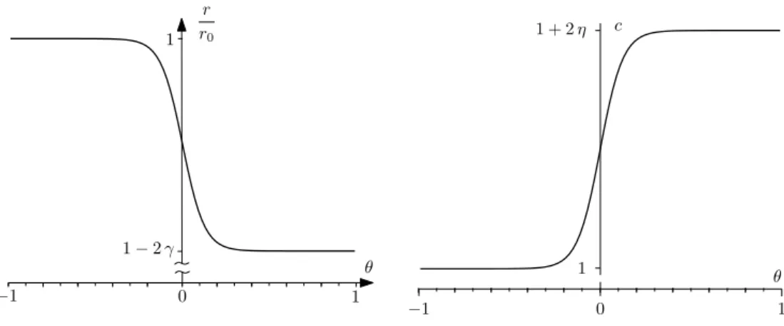
their dependence on temperature is negligible in an idealised sense. With this in mind, as an illustrative example we set
F =F(T) = 1 + tanh(λ θ) (138)
in the general results derived last subsection. Namely, we take into account the following forms of yield stress r=r(T) and Prager’s modulus c=c(T) as well as thermoinducer ϱ=ϱ(T):
r r0
= 1−γ(1 + tanh(λ θ)), (139)
c c0
= 1 +η(1 + tanh(λ θ)), (140)
ϱ ϱ0
= 1−ρ(1 + tanh(λ θ)). (141)
Herein, λ, γ, η and ρ are positive dimensionless constitutive constants. Of them, λ is greater than 1, so that each quantity displays a thermosensitivity property merely within temperature range [T0, T1]. Specifically, we have
λ >1, 0< γ < 1
2, η >− 1
2, 0< ρ < 1 2.
The property for the above three functions is shown in Figs. 1 and 2. It may be seen that each function displays the general property mentioned be-fore. Note that both the yield stressr and the thermoinducerϱmonotonically decrease with increasing temperature, whereas Prager’s modulus c increases with increasing temperature. Their rates of changing with temperature are characterised by the parameters γ,η and ρ.
The derivatives of r andϱ are given by r′
r0
=−ξ γ
(cosh(λ θ)2 , ϱ′ ϱ0
=−ξ ρ
1−2γ 1
−1 0 1
r r0
θ
Figure 1: Monotonically decreasing yield stressr(T) (and, similarly, ther-moinducerϱ(T))
1 + 2η
1
θ
−1 0 1
c
Figure 2: Monotonically increasing Prager’s modulusc(T)
Here ξ= 2λ/(T1−T0)>0. Hence, we have
−r′−√1.5τ00ϱ′=ξ
γ r0+√1.5ρ τ00 (cosh(λθ))2 ,
r′−√1.5τ0ϱ′=ξ−γ r0+
√
1.5ρ τ0
(cosh(λθ))2 .
Evidently, the former is always positive, and the latter is also positive whenever
√
1.5ρτ00 r0
> γ . (142)
Now we derive the results for the two-way plastic flow for the constitutive quantities introduced. First, from condition (121)1 we infer
√
1.5τ00 r0
(
1−ρ−ρ tanh(λθˆh
)
−√1.5α0 r0
=γ(1 + tanh(λθˆh)
)
−1. (143)
Then, the start temperature ˆθh of the plastic flow at heating is given by (cf.
eq. (128))
tanh(λθˆh) =
1 +√1.5τ00−α0 r0 γ+√1.5ρτ00
r0
Since |tanhx| ≤1 for any real numberx, such a solution is possible whenever
−1≤√1.5τ00 −α0
r0 ≤
2γ−1 + 2√1.5ρτ00 r0
. (145)
Besides, τ00 and α0 should also be restricted by condition (47), i.e.
√
1.5|τ00−α0|
r0 ≤
1. (146)
Next, from condition (122)1 and eqs. (139)–(141) we deduce
√
1.5ρτ00 r0
(tanhλ−tanh(λ θc)) = 2−2γ−γ(tanhλ+ tanh(λθc)). (147)
From this we infer that the start temperature θc of plastic flow at cooling is
given by (cf. eq. (129))
tanh(λ θc) =
√
1.5ρτ00 r0 +γ
√
1.5ρτ00 r0 −γ
tanhλ+ √2 (γ−1)
1.5ρτ00 r0 −γ
. (148)
The condition for such a solution is as follows:
(√
1.5ρτ00 r0
+γ
)
tanhλ−2 (1−γ) < √
1.5ρτ00 r0 −
γ .
Forλ≫1, we have tanhλ= 1. Then, the latter produces
√
1.5ρτ00 r0
>1−γ . (149)
Since γ < 12, condition (142) is implied by the above condition. Moreover, by using condition (149) we infer that condition (145) is implied by condi-tion (146). From these it follows that condicondi-tions (142), (145), (146) and (149) may be reduced to
√
1.5τ00 r0
> 1−γ ρ ,
√
1.5|τ00 −α0|
r0 ≤
1. (150)
With the two start temperatures ˆθh (i.e. ˆTh) and θc (i.e. Tc), strain
re-sponses can be determined for plastic flow induced at heating and cooling. Results are as follows (cf. eqs. (132) and (133)):
h∗ =β(T −T0)I+ (|h0| −ϕ(θ)) [h∗0], (151)
ϕ(θ) = √ 2 3 r0 c0 1 η (√
1.5ρτ00 r0
+γ
)
ln 1 +η(1 + tanh(λθ)) 1 +η(1 + tanhλθˆh)
for the plastic flow at heating, and
h∗=β(T−T0)I + (|h0| −h2W−φ(θ)) [h∗0], (152)
φ(θ) = √
2 3
r0
c0
1 η
(√
1.5ρτ00 r0 −
γ
)
ln 1 +η(1 + tanh(λ θ)) 1 +η((1 + tanh(λ θc))
, θ∈[−1, θc],
for the plastic flow at cooling. In the above, the maximal two-way strain change h2W is given by (cf. eq. (134))
h2W =ϕ(1) =
√ 2 3
r0
c0
1 η
(√
1.5ρτ00 r0
+γ
)
ln 1 +η(1 + tanhλ) 1 +η(1 + tanh(λθˆh)
). (153)
Moreover, condition (118) for a strain cycle is of the form:
ϕ(1) +φ(−1) = 0, namely (cf. eq. (135)),
(√
1.5ρτ00 r0 +γ
)
ln 1 +η(1 + tanhλ) 1 +η(1 + tanh(λθˆh)
) =
(√
1.5ρτ00 r0 −
γ
)
ln1 +η(1 + tanhθc)
1 +η(1−tanhλ) . (154)
From the conditions given by eq. (150), it may be seen that both the initial stress τ0 and the initial back stress α0 should be suitably generated to ensure
two-way memory effects. It is noted that sometimes processes of “ training” may be introduced for this purpose.
With four dimensionless parametersγ,η,ρandc0/r0, the three constitutive
quantities given by eqs. (139)–(141) are broad enough to describe two-way memory effects. Of them,c0 may be used to control the amount of the maximal
two-way strain change h2W, while the other three may be used to match the
two start temperatures ˆTh and Tc as well as the cyclic condition (140). In
addition, the initial values τ0 and α0 should be suitably chosen to meet the
conditions given by eq. (150). Further results and numerical examples will be presented next section.
7
Determination of parameters and numerical
ex-amples
The two-way memory effect is characterised by the two start temperatures ˆ