Terrain surfaces and 3-D landcover classification from small footprint full-waveform lidar data: application to badlands

(1)

HESSD

6, 151–205, 2009

3-D landcover classification from full-waveform lidar

F. Bretar et al.

Title Page

Abstract Introduction

Conclusions References

Tables Figures

◭ ◮

Back Close

Full Screen / Esc

Printer-friendly Version

Interactive Discussion

Hydrol. Earth Syst. Sci. Discuss., 6, 151–205, 2009 www.hydrol-earth-syst-sci-discuss.net/6/151/2009/ © Author(s) 2009. This work is distributed under the Creative Commons Attribution 3.0 License.

Hydrology and Earth System Sciences Discussions

Papers published inHydrology and Earth System Sciences Discussionsare under

open-access review for the journalHydrology and Earth System Sciences

Terrain surfaces and 3-D landcover

classification from small footprint

full-waveform lidar data: application to

badlands

F. Bretar1, A. Chauve1,2, J.-S. Bailly2, C. Mallet1, and A. Jacome2

1

Inst. G ´eographique National, Laboratoire MATIS, 4 Av. Pasteur, 94165 Saint-Mand ´e, France

2

Maison de la T él éd étection, UMR TETIS AgroParisTech/CEMAGREF/CIRAD, 500 rue J.F Breton, 34095 Montpellier, France

Received: 6 October 2008 – Accepted: 20 October 2008 – Published: 6 January 2009

Correspondence to: F. Bretar (frederic.bretar@ign.fr)

(2)

HESSD

6, 151–205, 2009

F. Bretar et al.

Title Page

Tables Figures

◭ ◮

Back Close

Full Screen / Esc

Abstract

This article presents the use of new remote sensing data acquired from airborne full-waveform lidar systems. They are active sensors which record altimeter profiles. This paper introduces a set of methodologies for processing these data. These techniques are then applied to a particular landscape, the badlands, but the methodologies are

5

designed to be applied to any other landscape. Indeed, the knowledge of an accu-rate topography and a landcover classification is a prior knowledge for any hydrological and erosion model. Badlands tend to be the most significant areas of erosion in the world with the highest erosion rate values. Monitoring and predicting erosion within badland mountainous catchments is highly strategic due to the arising downstream

10

consequences and the need for natural hazard mitigation engineering. Additionaly, be-yond the altimeter information, full-waveform lidar data are processed to extract inten-sity and width of echoes. They are related to the target reflectance and geometry. Wa will investigate the relevancy of using lidar-derived Digital Terrain Models (DTMs) and to investigate the potentiality of the intensity and width information for 3-D landcover

15

classification. Considering the novelty and the complexity of such data, they are pre-sented in details as well as guidelines to process them. DTMs are then validated with field measurements. The morphological validation of DTMs is then performed via the computation of hydrological indexes and photo-interpretation. Finally, a 3-D landcover classification is performed using a Support Vector Machine classifier. The introduction

20

of an ortho-rectified optical image in the classification process as well as full-waveform lidar data for hydrological purposes is then discussed.

1 Introduction

Remote sensing is an effective set of techniques to collect physical data from the Earth

surface used as inputs in erosion/hydrological models or to monitor hydrological fields

25

(3)

HESSD

6, 151–205, 2009

F. Bretar et al.

Title Page

Tables Figures

◭ ◮

Back Close

Full Screen / Esc

visible domain with optical sensors can be analyzed for generating 2-D landcover and landform maps either automatically by image processing methods (Chowdhury et al., 2007) or by photo-interpretation. The use of the infrared channel helps to detect the vegetation (Lillesand and Kiefer, 1994). In a stereoscopic configuration, images are processed to generate Digital Surface Models (DSMs) (Kasser and Egels, 2002).

5

More recently, airborne lidar (LIght Detection And Ranging) systems (ALS) provide 3-D point clouds of the topography by direct time measurement of a short laser pulse after reflection on the Earth surface. Moreover, such active systems, called “multiple echo lidar”, allow to detect several return signals for a single laser shot. It is particu-larly relevant in case of vegetation areas since a single lidar survey allows to acquire

10

not only the canopy top (the only visible layer from passive sensors), but also points inside the vegetation layer and on the ground underneath. Depending on the vegeta-tion density, some of them are likely to belong to the terrain. After a classificavegeta-tion step

in ground/off-ground points (also called filtering process), relevant Digital Terrain

Mod-els (DTMs) can be generated. Such DTMs are of high interest for geomorphologists

15

to study erosion processes (McKean and Roering, 2004) or to map particular land-forms (James et al., 2007). Moreover, hydrologic models such as TOPOG (O’Loughlin, 1986) or TOPMODEL (Quinn et al., 1991) handle topographic data either as Digital

Surface/Terrain Models or as meshes. By classifying terrain under different levels and

types of vegetation cover, lidar data, if suitable, could provide new land classification,

20

i.e., terrain, cover maps. This new 3-D landcover classification can even be more re-lated to the hydrological processes that are usually modelled in hydrological production

indices as the SCS runoffcurve number (USD, 1986), the runoffcoefficient in the

ra-tional method (Pilgrim, 1987) or the the plant cover factor in Wischmeier and Smith’s Empirical Soil Loss Model (USLE) (Wischmeier et al., 1978). Lidar data have also been

25

(4)

HESSD

6, 151–205, 2009

F. Bretar et al.

Title Page

Tables Figures

◭ ◮

Back Close

Full Screen / Esc

heights are then converted into friction coefficients.

Finally, multiple echo lidar data are typically used for the unique possibility of ex-tracting terrain points as well as vegetation heights with high accuracy. When suitable, Hollaus et al. (2005) insist on the possibility to derive the roughness of the ground from lidar point clouds. However, the filtering algorithm used to process lidar data is

land-5

scape dependent and the classification result may be altered (Sithole and Vosselman, 2004).

Based on the same technology than multiple echo lidar systems, full-waveform li-dar systems provide altimeter profiles of the reflected pulse. They represent the laser backscattered energy as a function of time. These profiles are processed to extract 3-D

10

points (echoes) but in addition, other interesting features that could be related to land-scape characteristics. Depending on the landland-scape properties (geometry, reflectance)

and on the laser diffraction angle (entailing small or large footprint), the recorded

wave-form becomes of complex shape. An analytical modelling of the profiles provides the 3-D position of significant targets as well as the intensity and the width of lidar echoes

15

(Sect. 3.1). A detailed state-of-the-art of such systems can be found in Mallet and Bretar (2009).

This paper introduces a set of methodologies for processing full-waveform lidar data. These techniques are then applied to a particular landscape, the badlands, but the methodologies are designed to be applied to any other landscape.

20

Indeed, badlands tend to be among the most significant areas of erosion in the world, mainly in semi-arid areas and in sub-humid Mediterranean mountainous areas (Torri and Rodolfi, 2000). For the latter case, more active dynamics of erosion are observed (Regues and Gallart, 2004) with the highest erosion rate values in the world

(Walling, 1988). Very high concentrations of sediment during floods, up to 1000 g l−1,

25

were registered (Descroix and Mathys, 2003).

(5)

HESSD

6, 151–205, 2009

F. Bretar et al.

Title Page

Tables Figures

◭ ◮

Back Close

Full Screen / Esc

1995). These landscapes result from unconsolidated sediments or poorly consolidated bedrock, as marls, under various climatic conditions governing bedrock disintegration

through chemical, thermal or rainfall effects (Nadal-Romero et al., 2007).

The hydrological consequences of erosion processes on this type of landscapes are a major issue for economics, industry and environment: high solid transport,

bring-5

ing heavily loaded downstream flood, are silting up reservoirs (Cravero and Guichon, 1989) and downstream river aquatic habitats (Edwards, 1969). Therefore, monitoring and predicting erosion within badland mountainous catchments is highly strategic due to the arising downstream consequences and the need for natural hazard mitigation engineering (Mathys et al., 2003). Traditionaly, the monitoring activities in catchments

10

are derived from heavy in situ equipments on outlets or from isolated and ponctual observations within catchments. In complement to these traditional observations, hy-drologists are expecting remote sensing to help them to upscale and/or downscale erosion processes and measurements in other catchments, by providing precise and continuous spatial observations of erosion features or erosion driven factors (Puech,

15

2000). Among other inputs, erosion monitoring and modelling approaches on badlands (Mathys et al., 2003) need maps of landform features, mainly gullies (James et al., 2007) that are driving the way flows and maps of important driven factors of erosion in mountainous badland catchments. These factors are soil and rocks characteristics (Malet et al., 2003), vegetation strata used to derive 3-D landcover classes controlling

20

rainfall erosivity, and the terrain topography (Zhang et al., 1996), which allow to derive slope and aspect of marly hillslopes (Mathys et al., 2003).

This paper aims at investigating the potentialities of using full-waveform lidar data as relevant altimeter data, but also as a possible data source for 3-D landcover tion focusing on the characterization of badland erosion features and terrain

classifica-25

(6)

HESSD

6, 151–205, 2009

F. Bretar et al.

Title Page

Tables Figures

◭ ◮

Back Close

Full Screen / Esc

Considering their novelty and their complexity, we propose to develop some new and specific guidelines related to their processing (including some physical corrections) and their management. Furthermore, we will show that DTMs generated from lidar data are of high accuracy, even over complex mountainous landscapes, which is consistent with the study of erosion processes. Finally, the extraction of the intensity and the width of

5

each echo is investigated as potential information for landcover classification. Intensity and width are related to the target reflectance as well as to the local geometry (slope, 3-D distribution of the target).

This paper begins with a background on full-waveform lidar systems (Sect. 2.1) as well as a brief presentation of a management system to handle the data (Sect. 2.2). We

10

then present the processes to convert raw data into 3-D point clouds (Sect. 3.1). Sec-tion 3.2 is dedicated to the development of a filtering algorithm to classify the lidar point

cloud into ground/off-ground points as well as on the generation of DTMs. The echo

intensity and width extracted from full-waveform lidar data are described in Sect. 3.3. We focus this section on theoretical developments, basis of the introduction of intensity

15

corrections. Section 4 presents the badland area whereon investigations have been performed as well as the data: lidar data, orthoimages and field measurements. DTMs produced by our algorithm are then validated by both field measurements (Sect. 5.1) and by the computation of an hydrological index (Sect. 5.2) compared with manually (photo-interpretation) extracted crests and thalwegs. We finally present in Sect. 6 the

20

results of a 3-D landcover classification using a first level of terrain vegetation cover classes and based on a supervised classifier: the Support Vector Machines (SVMs).

Different features have been tested, including the three visible channels of the

orthoim-age. The opportunity of using full-waveform lidar data for hydrological purposes is then discussed.

(7)

HESSD

6, 151–205, 2009

F. Bretar et al.

Title Page

Tables Figures

◭ ◮

Back Close

Full Screen / Esc

2 Managing full-waveform lidar data

2.1 Background on full-waveform lidar systems

The physical principle of ALS consists in the emission of short laser pulses, with a width of 5–10 ns at Full-Width-at-Half-Maximum (FWHM), from an airborne platform with a high temporal repetition rate of up to 200 kHz in multiple echo mode. They provide

5

a high point density and an accurate altimeter description within each laser diffraction

beam. The two way runtime to the Earth surface and back to the sensor is measured. Then, the range from the lidar system to the illuminated surface is recorded (Baltsavias, 1999). A lidar survey is composed of several parallel and overlapping strips (100 m to 1000 m width).

10

The emitted electromagnetic wave interacts with objects depending on its wave-length. The main influences on the laser light come from artificial or natural objects belonging to the illuminated surface. For ALS systems, near infra-red sensors are used (typical wavelengths from 0.8 to 1.55 µm). The Pulse Repetition Frequency (PRF) de-pends on the acquisition mode and on the flying altitude. Contrary to multiple echo

15

systems which record only some high energy peaks in real time, full-waveform lidar systems record the entire signal of the backscattered laser pulse. Figure 1 shows raw full-waveform data.

Full-waveform systems sample the received waveform of the backscattered pulse at a frequency of 1 GHz. The footprint size depends on the beam divergence and on the

20

flight altitude. Most commercial airborne systems are small footprint (typically 0.3 to

1 m diameter at 1000 m altitude).

2.2 Handling full-waveform lidar data

Initially, raw full-waveform lidar data are sets of range profiles of various lengths. Raw profiles are acquired and stored in the sensor geometry following both the scan angle

25

(8)

georefer-HESSD

6, 151–205, 2009

F. Bretar et al.

Title Page

Tables Figures

◭ ◮

Back Close

Full Screen / Esc

encing process and the pre-processing step (Sect. 3.1), raw profiles become vectors of attributes containing, for each 3-D point, the x-, y-, z-coordinates, additional param-eters (intensity and FWHM) and a link to the sensor geometry. Managing these data is much more complex than images: the topology (neigbhorhood system, topological

queries) is designed to be as efficient as possible when accessing and storing the data.

5

Indeed, the data volume is drastically larger than traditional laserscanning techniques: it takes 140 GB for an acquisition time of 1.6 h with a PRF of 50 kHz. Moreover, a 3-D/2-D visualization tool is also necessary to handle the attributes, both in the sensor and in the ortho-rectified geometries (cf. Fig. 2). A specific software has therefore been developed for these purposes.

10

3 Processing full-waveform lidar data

3.1 From 1-D signals 3-D to point clouds

Contrary to multiple echo lidar sensors which provide directly 3-D point clouds, full-waveform sensors acquire 1-D depth profiles along the line of sight for each laser shot. The derivation of 3-D points from these signals is composed of two steps:

15

– The waveform processing step provides the signal maxima location, i.e., the range

values, as well as additional parameters describing the echo shape.

– The georeferencing process turns the range value to a _{x, y, z} triplet within

a given geographic datum.

Waveform processing:It aims at maximizing the detection rate of relevant peaks within

20

the signal in order to foster information extraction. In the literature, a parametric ap-proach is generally chosen to fit the waveform. Parameters of a mathematical model are estimated. The objective is twofold. A parametric decomposition gives the signal

maxima, i.e., the range values of the different targets hit by the laser beam. Then, the

best fit to the waveform is chosen among a class of functions. This allows to introduce

(9)

HESSD

6, 151–205, 2009

F. Bretar et al.

Title Page

Tables Figures

◭ ◮

Back Close

Full Screen / Esc

new parameters for each echo and to extract additional information about the target shape and its reflectance.

Our methodology is based on a paper written by Chauve et al. (2007). The au-thors describe an iterative waveform processing using a Non-Linear Least Squares fitting algorithm. After an initial coarse peak detection, missing peaks are found in the

5

residuals of the difference between the modelled and initial signals. If new peaks are

detected, the fit is performed again. This process is repeated until no further improve-ment is possible. This enhanced peak detection method is useful to model complex waveforms with overlapping echoes and also to extract weak echoes.

The Gaussian function has been shown to be suitable to model echoes within the

10

waveforms (Wagner et al., 2006). Its analytical expression is:

fG(x)=Iexp −

|x₋µ_|2

2σ2 !

(1)

whereµis the maximum location,I the peak amplitude, andσthe peak width.

For each recorded waveform, the transmitted pulse is also digitized. By retrieving its maximum location, the time interval between the pulse emission and its impact

15

on a target is known. The range value of the target ensues from the time-of-flight calculation.

In this paper, the echo amplitude will be refered to as intensity. However, in the

literature, the intensity can also be associated to the total energy of the echo, product

of the intensity and σ. The standard deviation σ corresponds to the half width of the

20

peak at about 60% of the full height. In some applications, however, the

Full-Width-at-Half-Maximum (FWHM) is often used instead. We have FWHM=2σ√2 ln 2.

Georeferencing: Similarly to multiple echo lidar sensors, computing the _{x, y, z_} co-ordinates of each echo in a geodetic reference frame from the range value requires

additional data. The scan angle is used jointly to the range to calculate the _{x, y, z_}

25

(10)

HESSD

6, 151–205, 2009

F. Bretar et al.

Title Page

Tables Figures

◭ ◮

Back Close

Full Screen / Esc

recovered from the full-waveform data file to calculate the_{x, y, z} in a given

geode-tic datum. Finally, the positions can be transformed in some cartographic projection (French NTF Lambert II Etendu in this paper, see Sect. 4 for more details).

The transformation formulas cannot be expressed because they differ from a sensor

to another. Offset values are different, depending on the configuration of the laser

5

system, GPS and Inertial Measurement Unit (IMU) devices.

After applying the advanced step of waveform modelling, full-waveform lidar data generate denser point clouds than multiple echo data. It is particularly relevant when studying the vegetation structure (Mallet and Bretar, 2009). However, we will see in Sect. 6 that additional parameters are also of interest for landcover or soil classification.

10

3.2 From point clouds to DTM

The processing of a lidar point cloud consists in classifying the data, which is gener-ally associated to the resampling of the data on a regular grid. Due to the very fine geometry of a lidar point cloud, many algorithms have been developed to

automat-ically separate gound points from off-ground points (Sithole and Vosselman, 2004).

15

Most of these approaches have good results when the topography is regular, but re-main unperfect in case of mixed landscapes and slope conditions: parameters of the

algorithms are often difficult to tune and do not fit over a large area. When ground

points are mis-classified as off-ground points, the accuracy of the DTM may decrease

(it depends on the spatial resolution and on the interpolation method). Inversely, when

20

off-ground points (vegetation or man-made objects) are considered as ground points,

the DTM becomes spiky which can be mis-interpreted by hydrological models. Vege-tated landscapes with sparse vegetation in a mountainous areas (alpine landscapes) are particularly interesting for the study of natural hydrology and the phenomenoms of erosion (cf. Sect. 4). Nevertheless, the processing of such landscapes need strong

25

(11)

HESSD

6, 151–205, 2009

F. Bretar et al.

Title Page

Tables Figures

◭ ◮

Back Close

Full Screen / Esc

not explicitly introduced in the process.

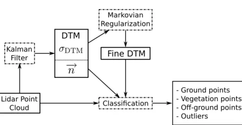
A methodology that handles these problems has been recently developed (Bretar and Chehata, 2008) and is used in this study to compute the DTMs. It is based on a two step process:

i. The computation of an initial surface using a predictive Kalman filter: it aims at

5

providing a robust surface containing low spatial frequencies of the terrain (main slopes). The algorithm consists in analyzing the altimeter distribution of the point cloud of a local area in the local slope frame. Points of the first altimeter mode (lowest points) belong to the terrain. A DTM value at a specific position depends on the neighboring pixels through their respective uncertainties. The predictive

10

Kalman framework provides not only a robust terrain surface (the slopes are also

integrated in the predictive filter), but also an uncertaintyσDTMfor each DTM pixel

as well as a map of normal vectorsn.

ii. The refinement of this surface using a Markovian regularization: it aims at

inte-grating micro relieves (lidar points within the uncertaintyσDTM) in a minimization

15

process to refine the terrain description. Formulated in a Bayesian framework, additional prior information (crest, thalweg etc.) can also be integrated in the refinement process.

The lidar point cloud is then classified based on geometric criteria. A lidar point is

labelled as “ground” if it is located within a buffer zone defined as the corresponding

20

DTM uncertainty σ_DTM. Otherwise, it is considered as “off-ground”. In natural

land-scapes, off-ground points belong mainly to vegetation, and sometimes to human-made

features (e.g., electric power lines, shelters). Vegetation areas are described as non-ordered point cloud (high variance) compared to human-made structures. Vegetation

points are therefore extracted by fitting a plane on the off-ground points. If the

resid-25

uals are higher than a defined threshold (_∼0.3 m), points are labelled as “vegetation”.

(12)

HESSD

6, 151–205, 2009

F. Bretar et al.

Title Page

Tables Figures

◭ ◮

Back Close

Full Screen / Esc

set related to the supervised classification (Sect. 6). Figure 4 is a 3-D bird view of the orthoimage superimposed on the DTM.

3.3 Processing intensity and width of lidar echoes

Beyond the 3-D point cloud, full-waveform lidar data provide intensity and width of each echo (Sect. 3.1) that are potential interesting features for landcover classification.

5

The backscattered intensity (or received power) is a function of the laser power, the distance source-target, the incidence angle, the target reflectivity, the absorption by the atmosphere etc. The use of such features in a landscape classification framework necessitates a global coherence between all strips. Correcting the recorded intensity values from some of known contributions makes possible the analysis of “physical”

10

parameters such as the target reflectivity. We propose also to analyze the effect of the

incidence angle on the Full-Width-at-Half-Maximum.

3.3.1 The intensity

According to Nicodemus et al. (1977), the scattered radiant fluxP_sin the zenith/azimuth

angles (θs, φs) within the cone Ωs is related to the incident flux Pi in the direction

15

(θ_i, φ_i) withinΩi by (Fig. 5)

P_s(θ_s, φ_s,Ωs)=̺(Ωi,Ωs)P_i(θ_i, φ_i,Ωi) (2)

where̺(Ωi,Ωs) is the biconical reflectance.

Introducing the backscattered cross section of the targetσ, Eq. (2) can be rewritten

as (Wagner et al., 2008b):

20

Ps = D2_r

4πR4_β2

t

σPi (3)

whereD_ris the diameter of the receptor,Rthe range from sensor to target,β_tthe laser

(13)

HESSD

6, 151–205, 2009

F. Bretar et al.

Title Page

Tables Figures

◭ ◮

Back Close

Full Screen / Esc

Withσ=πρ_mR2β2_tcosθ_s (H ¨ofle and Pfeifer, 2007)

P_s = D 2 rρm

4R2 cosθsPi (4)

whereρm is the target reflectance, which depends on the material.

Since the recorded intensity is proportional to the backscatterred flux Ps,

correct-ing intensity values gives access to the target reflectance, and therefore, in case of

5

a Lambertian surface, to the classification of the material. Since the apparent reflect-ing surface is smaller in case of non-zero incidence angle than in case of zenithal measurements (the cosinus dependency in Eq. 4), recorded intensity values are cor-rected from the scalar product of the emitted laser direction and the corresponding terrain local slope extracted from the DTM.

10

We have also remarked that emitted pulses have significant amplitude variations along the flight track which may alter the spatial homogeneity of returned waveforms. Figure 6a represents the ratio between the intensity values of the emitted laser pulse and the average intensity values over the whole strip along the flight track (x-axis). Considering the high PRF of the laser, intensity values are constant along the scan line.

15

The effects of such variations are visible in the returned waveforms as vertical lines

(Fig. 6b). We therefore normalized the returned waveforms by the average intensity

value of all emitted pulses. The effects of the correction are presented in Fig. 6c. One

can notice that vertical lines have disappeared.

3.3.2 The Full-Width-at-Half-Maximum

20

The FWHM has shown some spatial variability in our data set. Considering the bad-land and alpine bad-landscape, we investigated the influence of the incidence angle on the

FWHM only in case ofbare soil areas. Indeed, the FWHM of under-vegetation ground

points may have been modified by the complex optical medium. These investigations have been performed on simulated waveforms reflected by a tilted planar surface. We

25

(14)

HESSD

6, 151–205, 2009

F. Bretar et al.

Title Page

Tables Figures

◭ ◮

Back Close

Full Screen / Esc

the FWHM should stay constant with various incidence angles. We cannot extend this conclusion for ground points below the vegetation since the waveform has been mod-ified through the canopy cover. The spatial variability is therefore attributed to a more complex spatial beam response of the surface due to structures and/or reflectance properties.

5

4 Materials

Lidar data have been acquired over the Draix area, France. Draix area is an exper-imental area on erosion processes in badlands located in the South of the French Alps. It belongs to the Euromediterranean Network of Experimental and Representa-tive Basins (ERB). The Draix area consists in five research experimental catchments,

10

highly equipped and monitored for more than thirty years. Thirteen research units working on erosion and hydrology processes are grouped within the GIS Draix orga-nization (Mathys, 2004). Results for the most two eroded catchments are presented here: they concern the Laval and the Moulin catchments.

4.1 Lidar data

15

The data acquisition was performed in April 2007 by Sint ´egra (Meylan, France) using a RIEGL© LMS-Q560 system. This sensor is a small footprint airborne laser scanner and its main technical characteristics are presented in Wagner et al. (2006). The lidar system operated at a PRF of 111 kHz. The flight height was approximatively 600 m

leading to a footprint size of about 0.25 m. The point density was about 5 pts/m2.

20

The temporal sampling of the system is 1 ns. Each return waveform is made of one or two sequences of 80 samples. For each profile, a record of the emitted laser pulse is also provided (40 samples).

For this study, three overlapping strips have been used with perpendicular direction. For each of them, a sub-part corresponding to the Moulin and the Laval catchement

(15)

HESSD

6, 151–205, 2009

F. Bretar et al.

Title Page

Tables Figures

◭ ◮

Back Close

Full Screen / Esc

have been extracted. Strip footprints are presented in Fig. 8 and denoted S6 (blue), S7 (red), S8 (green).

4.2 Orthoimages

Two orthoimages were available for the study. The first one is extracted from the French IGN data basis BDOrtho©. Acquired in fairly good conditions (almost no shadowed

5

zones) by the IGN digital camera, a physical-based radiometric equalization process has been applied (Paparoditis et al., 2006). The ground resolution is 0.5 m. The triplet

of_{red, green, blue_} channels of the IGN image will be referred in this article to as

RGBIGN. The second orthoimage has been calculated from aerial images acquired

during the lidar survey by an embedded digital camera. Since the survey has been

10

performed early in the morning, numerous shadowed areas appear. Moreover, no radiometric equalization has been performed entailing a rather poor radiometric quality

(see Fig. 13). The ground resolution is 0.2 m. The triplet of_{red, green, blue_}channels

of this image will be referred in this article to as RGB_RAW.

4.3 Field measurements

15

Quality control points (or ground truth data) were surveyed by a mixed campaign DGPS, and a Total Station (coordinate reference system NTF Lambert II Etendu). The accuracy was 0.025 m in planimetry, and 0.03 m in altimeter. These points are chosen mainly on thalwegs (bottom of gullies) and crests. Some gullies are so deep that the GPS system was not able to work at the same accuracy. Those points were then

sur-20

(16)

HESSD

6, 151–205, 2009

F. Bretar et al.

Title Page

Tables Figures

◭ ◮

Back Close

Full Screen / Esc

5 DTMs analysis

5.1 Qualification of DTMs with field measurements

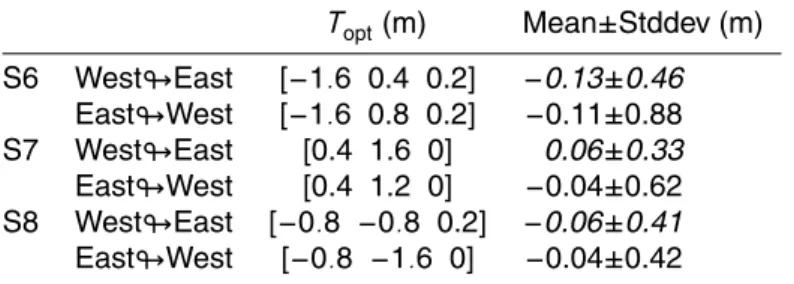
We present in Table 2 a comparison between field measurements and three DTMs generated from each single strip (S6, S7 and S8). One can observe that there is a bias in each DTM w.r.t. field measurements as well as a significant standard deviation and

5

RMS.

Looking carefully throught the lidar data and the statistics, a strip adjustment prob-lem was diagnosticated. In order to validate the DTMs, the West part of the field measurements has been used to adjust the DTM while the East part to validate the

terrain surface (denoted West#_{East in Table 1). We also took the dual configuration}

10

(East#_{West) to test the relevancy of the proposed correction. Here, the adjustement}

consists in finding the best 3-D translation Topt that minimizes a RMS between field

measurements and their projection on the DTM. We used a brute force method to

ex-plore the entire parameter space. A x, y (resp. z) search step of 0.4 m (resp. 0.1 m)

was chosen in relation to the planimetric (resp. altimeter) accuracy of lidar points. The

15

symmetrical validation gives some hints on the real deformations of the DTM, which are generally much more complex than a 3-D translation. Table 1 gathers the results of both the optimal correction applied to each DTM and the mean and standard deviation

of respectively West#_{East and East}#_{West configurations.}

Table 1 shows that the adjustement improves the final accuracy of DTMs both by

de-20

creasing the bias and the standard deviation. However, one can notice that the optimal

3-D translation varies depending on the West#_{East and East}#_{West configuration.}

A 0.4 m difference in the y-direction ofToptfor DTMs S7 and S6 doubles the standard

deviation, while a 0.8 m difference in the y-direction of Topt for DTM S8 has no effect

on the final accuracy. These observations tend to show that the deformations between

25

DTMs is not purely a 3-D translation, but is of different nature such as polynomial

(sur-face tilt) or non linear (rotation).

(17)

calcu-HESSD

6, 151–205, 2009

F. Bretar et al.

Title Page

Tables Figures

◭ ◮

Back Close

Full Screen / Esc

lated DTMs at 1 m resolution have an absolute altimeter accuracy of some decimeters. A better geometric adjustement should improve this accuracy.

5.2 Qualification of DTMs with hydrological indices and photo-interpretation

The quality assessment of a DTM for hydrological purposes is not completely satis-fying when considering only the altimeter error distribution. Other DTM quality

crite-5

ria directly connected to the usual hydrological information extracted from DTM may be used: drainage networks, drainage areas, slopes like presented in (Charleux-Demargne, 2001). These criteria are mainly based on the basic landform informa-tion related to the first and the second derivative of a DTM. However, these criteria are not easy to use in a qualification process since (1) they are conditioned by both

10

the algorithms and the parameters used to produce the information (e.g., a drainage area threshold in the D8 flow accumulation algorithm), (2) reference data are not easily available (how to survey drainage networks?) and finally (3) the quantification of quality is often not properly defined (how to compare dissimilarities of drainage networks?). Moreover, criteria are usually not generic: it is related to a specific hydrological index.

15

In order to overcome these problems, a single criteria is proposed for a quantified auto-evaluation of DTMs at a given resolution in erosion areas with an hydological and morphological point of view.

This criteria is the rate of crests and thalwegs observed from an orthoimage that are detected from the convergence index (CI) built on a DTM (K ¨othe and Lehmeier,

20

1994). The convergence index corresponds, for each DTM cell, to the mean difference

between angle deviations. These angle deviations are calculated in each of the eight

adjacent pixels. For an adjacent pixel, the angle deviation is the absolute difference, in

degrees, modulo 180, between its aspect and the azimuth to the central pixel (Zeven-bergen and Thorne, 1987). The convergence index is a symetric and continuous index

25

ranging from ₋90◦ up to 90◦. This index highlights crests when highly positive and

(18)

HESSD

6, 151–205, 2009

F. Bretar et al.

Title Page

Tables Figures

◭ ◮

Back Close

Full Screen / Esc

positive (red) values.

At a given location, a thalweg (resp. a crest) is considered to be detected in the

DTM) if CI values belong to [₋90◦,₋η] (resp. to [η,90◦], η_∈R). On a “perfect” DTM

without noise, only CI=0 (i.e., η=0) indicates a plane terrain without any crests and

thalwegs, whatever the slope is. When dealing with noisy DTM, thresholding the CI

5

with η to retrieve significant crests and thalwegs becomes a challenging task. We

therefore simulated a distribution of CI from a set of 1000 virtual noisy DTMs. They

were generated with a trend corresponding to a plane of constant slope (e.g., 33◦ is

the mean slope of Draix area). The simulation consists in generating Gaussian random fields (Lantuejoul, 2002) using the LU method (Journel and Huijbregts, 1978) following

10

noise spatial distribution models with parameters: range, nugget and sill (variance) for spatial covariance.

Since the simulated CI distribution is of Gaussian shape, we setηto two times the

standard deviation. We accept that five percents of CI values due to hazard on noise can be classified in significant crest and thalweg.

15

We show some results on a sub-aera of Draix. The simulated CI distribution

(per-formed on 33◦ slope, Gaussian noise of zero mean and 2.66 standard deviation)

pro-vides a threshold valueη=8.46. We show the results of the thalweg and crest detection

on Fig. 10.

Figure 10a is a manual delineation of apparent crests and thalwegs. The

photo-20

interpretation process is applied on main structures, but very close linear elements as well as the elements near sporadic vegetated elements are not considered.

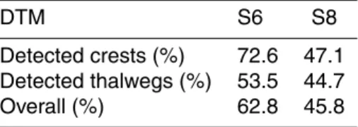
Table 3 presents the quality criteria for S6 and S8. The overall accuracy for S6 (resp. S8) is 62.8% (resp. 45.8%). These relatively low values can be explained by

the following grounds. Firstly, the thresholdηhas been automatically calculated: the

25

(19)

HESSD

6, 151–205, 2009

F. Bretar et al.

Title Page

Tables Figures

◭ ◮

Back Close

Full Screen / Esc

the DTM, they may not appear in the photo-interpreted features since they may either be located in shadowed areas (thalwegs) or in saturated bright areas (crests). The comparison is therefore biased.

Moreover, when comparing results for S6 and S8, results show that (1) S6 is bet-ter representing landforms than S8 probably due to georeferencing problems and

5

(2) crests are more precisely detected in DTMs than thalwegs, which has to be more deeply investigated.

5.3 Discussion

Regarding the altimeter quality of full-waveform LiDAR DTMs, we obtain a rather pre-cise and accurate relief restitution of a catchment of several square kilometers (about

10

the same as the one obtained with multi-echo LiDAR). However, we showed that

al-timetric criteria are not sufficient since some differences in the restitution of eroded

terrain features are observed between DTMs (coming from different strips). In

ad-dition, morphological criteria has necessary to be considered. The observation of local erosion processes requires a more detailed relief restitution. Other techniques

15

like terrestrial LiDAR or photogrammetry by unmanned aerial vehicles (Jacome et al., 2008) are more accurate and precise, but, are not well adapted to survey large ar-eas. However, considering the altimeter accuracy of DTMs (approximately 0.9 m for 2 standard deviation on the altimeter random error), and that the local ablation speed over Draix area is of 1.5 cm per year (Oostwoud and Ergenzinger, 1998), change

de-20

tection and monitoring of erosion effects would require a delay between surveys of

several decades. Nevertheless, the loss of sediment volume within catchments are not

homogeneous and are temporary stored on hill-slope gully networks: _∼200 tons/km2

are trapped in the gully network), which corresponds to an approximate of 150 m3

(Mathys et al., 1996). These volumes are significant enought to shorter time lag for

25

(20)

HESSD

6, 151–205, 2009

F. Bretar et al.

Title Page

Tables Figures

◭ ◮

Back Close

Full Screen / Esc

sediment volume displacement in the gully network at a catchments scale.

6 3-D landcover classification

6.1 Methodology

Lidar data have been used so far as accurate altimeter data to extract ground points and generate DTMs. The challenges were to automatically process the data in a

moun-5

tainous landscape with steep slopes and vegetation, the whole with the highest accu-racy. We mentionned in the introduction that a landcover map is an important input of hydrological models, especially for the parameterization of the hydrological produc-tion funcproduc-tion. We therefore propose in this secproduc-tion to describe the inputs and outputs of a classification framework wherein lidar width and intensity values can be integrated

10

and their benefit evaluated. Indeed, the interpretation of additional lidar parameters has been barely studied and reveals to be of interest for landcover classification. Wagner et al. (2008a) proposed classification rules based on a decision tree for vegetation/non-vegetation areas in a urban landscape using solely the width and the amplitude: a point

is considered asvegetationif (1) it is not the last pulse of a profile containing multiple

15

returns (2) it is a single return with low amplitude (_≤75) and large width (_≥1.9 ns).

Fo-cusing on the study of the vegetation, Reitberger et al. (2008) have integrated different

features to segment individual trees in a graph-cut framework. Among them, the au-thors show that the feature corresponding to the average intensity on the entire tree plays the most important role in leaf-on conditions, while the ratio between the

num-20

ber of single reflections and the number of multiple reflections is the most important in

leaf-offconditions.

Here, we would like to answer the question: do lidar width and intensity values

im-prove a classification pattern in badlands? An efficient supervised classification

algo-rithm called Support Vector Machines (SVM) has been used (Chang and Lin, 2001).

25

(21)

HESSD

6, 151–205, 2009

F. Bretar et al.

Title Page

Tables Figures

◭ ◮

Back Close

Full Screen / Esc

analysis (Huang et al., 2002): ability to mix data from different sources, robustness to

dimensionality, good generalization ability and a non-linear decision function (contrary to decision trees for instance). In this paper, the 3-D lidar point cloud is labelled, thus providing a 3-D landcover classification. (Mallet et al., 2008) applied this technique with success for classifying urban areas from full-waveform lidar data.

5

Four classes have been identified focusing on a first and simple hierarchical level of 3-D land cover classification, relevant for badlands landscapes with anthropogenic

elements: 1-land, 2-road, 3-rock and 4-vegetation. The three first classes can be

ordered on an increasing erosion sensitivity criteria. The first classland is taking into

account terrain under natural vegetation cover and cultivated areas in grassland. The

10

second one, roads, are linear elements with natural (marls), bared but compacted

material. These elements are known to impact runoff production within catchments.

The third one contains areas with bared black marls in gullies, the main source of sediment production. The latter, vegetation, could be used further to describe the 3-D vegetation structure, useful for a more detailed hierarchical level of 3-D land cover

15

classification.

SVM algorithm requires its own feature vector for each 3-D lidar point to be classified. Only three lidar features have been retained. Indeed, it appears that the larger the

number of features, the more difficult to make an interpretation of the results. They are:

– dDTM, the distance between the 3-D point and the DTM,

20

– Int, the echo intensity,

– FWHM, the echo width (see Sect. 3.1).

Additionally, the RGBIGNand RGBRAWfeatures have been added in the classifier,

pro-viding three radiometric attributes (Fig. 12). Their introduction allows a discrimination between road and land impossible with the lidar features and improve the classification

25

(22)

HESSD

6, 151–205, 2009

F. Bretar et al.

Title Page

Tables Figures

◭ ◮

Back Close

Full Screen / Esc

– road androck: 200 lidar points are selected in a road and rock mask defined on

the orthoimage.

– vegetation: 200 lidar points are selected within a vegetation mask (lidar points classified as vegetation in Sect. 3.2)

– land: 200 lidar points are selected (1) in a land mask on the orthoimage (2) in the

5

intersection of the vegetation mask and a ground mask (lidar points classified as ground in Sect. 3.2).

We have implemented the SVM algorithm with the LIBSVM software (Hsu and Lin,

2001), selecting the generic Gaussian kernel. For more theoretical explanations,

please see (Pontil and Verri, 1997).

10

6.2 Results and discussion

The data set S6 has been analyzed. Figure 11 shows the histograms of lidar derived

features corresponding to the four selected classes.dDTMand Int have bounded values

which describe the vegetation (resp.>1 m and between 0 and 20), whereas the width

values tend to be uniform between 3 ns and 4.5 ns. road andland have similar

distri-15

butions for lidar derived features, which explains the high confusion values in Table 4.

The distributions of rock is flattened for dDTM since many points are choosen in very

steep slopes, and are therefore more sensitive to the DTM quality. The intensity ofrock

is slighty different from the other classes. Figures 12 and 13 show the histograms of

RGBIGN.

20

The classification is validated with lidar points belonging to the masks defined in

the training step, but the training points. ∼40% of the total number of points have been

validated. Figure 14 shows the four validation sets for each class. A confusion matrix is then calculated for each configuration. True positive values correspond to the diagonal values of the confusion matrix. The accuracy of the classification results are quantified

(23)

HESSD

6, 151–205, 2009

F. Bretar et al.

Title Page

Tables Figures

◭ ◮

Back Close

Full Screen / Esc

by the average accuracy AA, mean of the diagonal values of the confusion matrix.

AAdoes not depends on the number of points in each validation set.

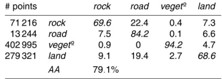
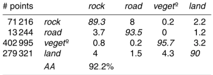
When using solely lidar derived features_{dDTM, Int, FWHM}, Table 4 indicates that

the confusion between classes is not negligible particularly for some of them: rock

withroad reaches 22.4%, while land with road reaches 19.4%, what was predictable

5

looking through the statistics of the training set (Fig. 11). The vegetation has a high percentage of true positive (94.2%) and is well detected. With an average accuracy of 79.1%, it appears that a classification based only on lidar derived features is consistent.

Before testing the effects of introducing lidar intensity and width, we investigated

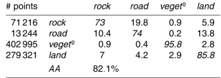
the impact of the radiometric quality of the orthoimages on the classification results.

10

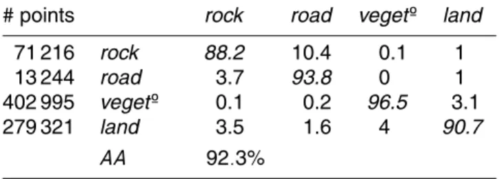
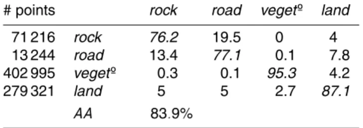
Tables 5 and 6 are the confusion matrices corresponding to the classification results

with, respectively{dDTM, RGBRAW} and {dDTM, RGBIGN}. One can observe a

signifi-cant discrepancy between both radiometric features with an average accuray of 82.1%

using_{dDTM, RGBRAW}and 92.2% using{dDTM, RGBIGN}. The true positive values of

rock (resp.road) increase from 73% (resp. 74%) to 89.3% (resp. 93.5%) when using

15

{dDTM, RGBIGN}instead of{dDTM, RGBRAW}. Moreover, the confusion between several

classes decreases significantly: road with rock decreases from 10.4% to 3.7%, road

withland from 13.8% to 1.2%, rock withroad from 19.8% to 8%,land withroad from

4.2% to 1.5%. In other words, the use of_{dDTM, RGBIGN}instead of {dDTM, RGBRAW}

gives better classification results.

20

True positive values are higher when using image-based features{dDTM, RGBIGN}

than _{dDTM, Int, FWHM} and the confusion between classes most of the time

de-creases:landwithroaddecreases from 19.4% to 1.5%,roadwithroaddecreases from

22.4% to 8%. Nevertheless, the comparison is more mitigated with{dDTM, RGBIGN}.

Indeed, true positive values ofroad decrease from 84.2% to 74% and the confusion

25

between the other classes increases significantly. However, land is better classified

with less confusion withroad (19.4% to 4.2%). As a result, it appears that even if the

(24)

HESSD

6, 151–205, 2009

F. Bretar et al.

Title Page

Tables Figures

◭ ◮

Back Close

Full Screen / Esc

The results of the introduction of lidar intensity and width in the classification

pro-cess are shown in Tables 7 and 8. There are minor effects on the results when using

{RGBIGN, Int, FWHM,dDTM}instead of{RGBIGN,dDTM}. The classification is bettered

when using _{RGBRAW, Int, FWHM, dDTM} instead of {RGBRAW, dDTM}, true positive

values ofrock increase from 73% to 76.2%,road increase from 74% to 77.1%,

vege-5

tationare similar andland increase from 85.8% to 87.1%. When comparing{RGBRAW,

Int, FWHM, dDTM} with{Int, FWHM, dDTM}(Table 4), the improvement is particularly

consistent forrock,land andvegetation, but true positive values ofroaddecrease from

84.2% to 77.1% and the confusion withrock increases from 7.5% to 13.4%. In fact,

the radiometry of roads are sensitive to tree shadows. The combination of the very

10

high resolution of RGB_RAW and the time of the survey (early in the morning) feeds the

training set with bright and dark (shadow) radiometric values. On the contrary, lidar intensity and width do not depend on the sun configuration. Superimposed on the

or-thoimage of Fig. 15, a 3-D landcover classification obtained with_{RGB_IGN, Int, FWHM,

dDTM}is presented in Figs. 16 and 17.

15

Finally, the quality of the classification depends mainly on the DTM accuracy

(repre-sented here asdDTM). Moreover, within the framework of the methodology, it appears

that a classification based on{Int, FWHM,dDTM}is suitable, but gives a worse

accu-racy than a classification based on_{dDTM, RGBRAW}or{dDTM, RGBIGN}. Used on their

own, full-waveform lidar data are relevant to discriminate vegetation from non

vege-20

tation points, but the confusion between other classes remains not negligible. The intensity and the width do not improve the classification accuracy if the radiometric fea-tures have a good separation between classes. Otherwise, the benefit is rather small, but in case of artefacts in a class (like shadow) for which lidar measurements are not sensitive. Inversely, the use of poor radiometric features may alter the classification

25

result of specific landscapes (hereroad) where intensity and width are well bounded.

(25)

HESSD

6, 151–205, 2009

F. Bretar et al.

Title Page

Tables Figures

◭ ◮

Back Close

Full Screen / Esc

For instance, these waveform parameters would probably give information on vegeta-tion density and type as well as local bared soil properties impacting laser reflectances. These investigations will be the next steps of our research.

7 Conclusions

The different points treated in this paper entail some conclusions. Firstly, the

accu-5

racy of the full-waveform lidar data we worked on (badlands) was proven decimetric. Even if erosion dynamics on these landscapes would require a centimetric accuracy to be studied yearly, DTMs generated from lidar survey are consistent for hydrologi-cal sciences at the catchment level. Moreover, we showed that these data permit to identify most of gullies and crests of badland landscapes through geomorphological

10

indices. We focused this paper on generating and qualifying DTMs, but also on the automatic computation of a 3-D landcover classification. We showed that lidar inten-sity and width contain enough discriminative information on badlands to be classified inland,road,rock andvegetationwith_∼80% accuracy. Compared to usual landcover classification from aerial or satellite images, 3-D landcover classification is a new and

15

interesting approach for hydrologists since it allows to parametrize in a much direct way hydrological or erosion production parameters as, for instance, the plant cover C factor (Wischmeier et al., 1978). However, the introduction of image-based radiometric features combined to lidar ones in the classifier improved the accuracy of the

classifi-cation (_∼92%). They bring relevant discrimination between classes but cancelled most

20

part of the value added from full-waveform data. This is mainly due to the generality of the landcover classes we chose, but it would probably be more discriminant for more detailed landcover classes.

Acknowledgements. The authors would like to deeply thank the GIS Draix for providing the full-waveform lidar data and for helping in ground truth surveys. They are grateful to INSU for

25

(26)

HESSD

6, 151–205, 2009

F. Bretar et al.

Title Page Abstract Introduction Conclusions References Tables Figures ◭ ◮ ◭ ◮ Back Close

Full Screen / Esc

References

United States Department of Agriculture (USD): Urban hydrology for small watersheds, Tech-nical Release 55, Natural Resources Conservation Service, Conservation Engineering Divi-sion, 2nd edn., 1986. 153

Antoine, P., Giraud, D., Meunier, M., and Ash, T. V.: Geological and geotechnical properties of

5

the Terres Noires in southeastern France: weathering, erosion, solid transport and instability, Eng. Geol., 40, 223–234, 1995. 154

Antonarakis, A. S., Richards, K. S., Brasington, J., Bithell, M., and Muller, E.: Retrieval of vegetative fluid resistance terms for rigid stems using airborne lidar, J. Geophys. Res., 113, G02S07, doi:10.1029/2007JG000543, 2008. 153

10

Bailly, J., Lagacherie, P., Millier, C., Puech, C., and Kosuth, P.: Agrarian landscapes linear features detection from LiDAR elevation profiles: application to artificial drainage network detection, Int. J. Remote Sens., 29(11–12), 3489–3508, 2008. 153

Baltsavias, E. P.: Airborne Laser Scanning: Basic relations and formulas, ISPRS J. Pho-togramm., 54(2–3), 199–214, 1999. 157

15

Bretar, F. and Chehata, N.: Terrain Modelling from lidar range data in natural landscapes: a predictive and Bayesian framework, Tech. rep., Institut G ´eographique National, available at http://hal.archives-ouvertes.fr/hal-00325275/fr/, 2008. 161

Bryan, R. and Yair, A.: Perspectives on studies of badland geomorphology, in: Badland Geo-morphology and Piping, edited by Bryan R. Y. A., GeoBooks (Geo Abstracts Ltd), pp. 1–12,

20

Norwich, UK, 1982. 154

Chang, C.-C. and Lin, C.-J.: LIBSVM: a library for support vector machines, software available at http://www.csie.ntu.edu.tw/∼cjlin/libsvm, 2001. 170

Charleux-Demargne, J.: Qualit é des mod èles num ériques de terrain pour l’hydrologie. Applica-tion à la caract érisaApplica-tion du r égime de crues des bassins versants, Ph.D. thesis, Universit é

25

de Marne-La-Vall ´ee, France, 2001. 167

Chauve, A., Mallet, C., Bretar, F., Durrieu, S., Pierrot-Deseilligny, M., and Puech, W.: Process-ing full-waveform lidar data: modelProcess-ing raw signals, in: IAPRS, vol. 36 (Part 3/W52), Espoo, Finland, 2007. 159

Chowdhury, P. R., Deshmukh, B., and Goswami, A.: Machine Extraction of Landforms from

Mul-30

(27)

HESSD

6, 151–205, 2009

F. Bretar et al.

Full Screen / Esc

Interactive Discussion 153

Cobby, D. M., Mason, D. C., and Davenport, I. J.: Image processing of airborne scanning laser altimetry data for improved river flood modelling, ISPRS J. Photogramm., 56(2), 121–138, 2001. 153

Cravero, J. and Guichon, P.: Exploitation des retenues et transport des s ´ediments, La Houille

5

Blanche, 3–4, 292–296, 1989. 155

Descroix, L. and Mathys, N.: Processes, spatio-temporal factors and measurements of current erosion in the French Southern Alps: a review, Earth Surf. Proc. Land., 28(9), 993–1011, 2003. 154

Edwards, D.: Some effects of siltation upon aquatic macrophyte vegetation in rivers,

Hydrobi-10

ologia, 34(1), 29–38, 1969. 155

H ¨ofle, B. and Pfeifer, N.: Correction of laser scanning intensity data: Data and model-driven approaches, ISPRS J. Photogramm., 62(6), 415–433, 2007. 163

Hollaus, M., Wagner, W., and Kraus, K.: Airborne laser scanning and usefulness for hydrologi-cal models, Adv. Geosci., 5, 57–63, 2005,

15

http://www.adv-geosci.net/5/57/2005/. 154

Hsu, C.-W. and Lin, C.-J.: LIBSVM: a library for Support Vector Machine, software available at http://www.csie.ntu.edu.tw/∼_{cjlin/libsvm, 2001. 172}

Huang, C., Davis, L., and Townshend, J.: An assessment of support vector machines for land cover classification, Int. J. Remote Sens., 22(4), 725–749, 2002. 171

20

Jacome, A., Puech, C., Raclot, D., Bailly, J. S., and Roux, B.: Extraction d’un mod èle num érique de terrain à partir de photographies par drone, Revue des Nouvelles Technologies de l’Information, E(13), 108–121, 2008. 169

James, L., Watson, D., and Hansen, W.: Using LiDAR data to map gullies and headwater streams under forest canopy: South Carolina, USA, CATENA, 71(1), 2007. 153, 155

25

Journel, A. and Huijbregts, C.: Mining Geostatistics, Academic Press, London, 1978. 168 Kasser, M. and Egels, Y.: Digital Photogrammetry, Taylor & Francis, 2002. 153

King, C., Baghdadi, N., Lecomte, V., and Cerdan, O.: The application of Remote Sensing data to monitoring and modelling of soil erosion, CATENA, 62(2–3), 79–93, 2005. 152

K ¨othe, R. and Lehmeier, F.: SARA System – System zur Automatischen Relief-Analyse, 1994.

30

167

(28)

HESSD

6, 151–205, 2009

F. Bretar et al.

Full Screen / Esc

Interactive Discussion Lillesand, T. and Kiefer, R.: Remote Sensing and Image interpretation, John Wiley & Sons,

1994. 153

Malet, J., Auzet, A., Maquaire, O., Ambroise, A., Descroix, L., Esteves, M., Vandervaere, J., and Truchet, E.: Investigating the influence of soil surface characteristics on infiltration on marly hillslopes, Earth Surf. Proc. Land., 28(5), 547–560, 2003. 155

5

Mallet, C. and Bretar, F.: Full-Waveform Topographic Lidar: State-of-the-Art, ISPRS J. Pho-togramm., submitted, 2009. 154, 155, 160

Mallet, C., Bretar, F., and Soergel, U.: Analysis of full-waveform lidar data for classification of urban areas, Photogrammetrie Fernerkundung GeoInformation (PFG), 5/2008, 337–349, interne, 2008. 171

10

Mason, D. C., Cobby, D. M., Horritt, M. S., and Bates, P. D.: Floodplain friction parameteriza-tion in two-dimensional river flood models using vegetaparameteriza-tion heights derived from airborne scanning laser altimetry, Hydrol. Process., 17(9), 1711–1732, 2003. 153

Mathys, N.: Information available http://www.grenoble.cemagref.fr/etna/oreDraix/oreDraix.htm, 2004. 164

15

Mathys, N., Brochot, S., and Meunier, M.: L’ érosion des Terres Noires dans les Alpes du Sud : contribution l’estimation des valeurs annuelles moyennes (bassins versants exp érimentaux de Draix, Alpes-de-Haute-Provence, France), Revue de g éographie alpine, pp. 17–27, 1996. 169

Mathys, N., Brochot, S., Meunier, M., and Richard, D.: Erosion quantification in the small marly

20

experimental catchments of Draix (Alpes de Haute Provence, France). Calibration of the ETC rainfall-runoff-erosion model, CATENA, 50(2-4), 527–548, 2003. 155

McKean, J. and Roering, J.: Objective landslide detection and surface morphology mapping using high-resolution airborne laser altimetry, Geomorphology, 57(3–4), 331–351, 2004. 153 Murphy, P., Meng, J. O. F., and Arp, P.: Stream network modelling using lidar and

photogram-25

metric digital elevation models: a comparison and field verification, Hydrol. Process., 22(12), 1747–1754, 2008. 153

Nadal-Romero, E., Regu ´es, D., Marti-Bono, C., and Serrano-Muela, P.: Badland dynamics in the Central Pyrenees: temporal and spatial patterns of weathering processes, Earth Surf. Proc. Land., 32(6), 888–904, 2007. 155

30

(29)

HESSD

6, 151–205, 2009

F. Bretar et al.

Full Screen / Esc

Interactive Discussion O’Loughlin, E.: Prediction of surface saturation zones in natural catchments by topographic

analysis, Water Resour. Res., 22(5), 794–804, 1986. 153

Oostwoud, W. D. and Ergenzinger, P.: Erosion and sediment transport on steep marly hillslopes, Draix, Haute-Provence, France: an experimental field study, CATENA, 33(22), 179–200, 1998. 169

5

Paparoditis, N., Souchon, J.-P., Martinoty, G., and Pierrot-Deseilligny, M.: High-end aerial digital cameras and their impact on the automation and quality of the production workflow, ISPRS J. Photogramm., 60, 400–412, 2006. 165

Pilgrim, D. H. (Ed.): Australian rainfall and runoff, Institution of Engineers, Canberra, Australia, 1987. 153

10

Pontil, M. and Verri, A.: Properties of support vector machines, Tech. Rep. AIM-1612, MIT, Cambridge, USA, 1997. 172

Puech, C.: Utilisation de la t él éd étection et des mod èles num ériques de terrain pour la connais-sance du fonctionnement des hydrosyst èmes, Habilitation à diriger des recherches, Greno-ble University, 2000. 155

15

Quinn, P., Beven, K., Chevallier, P., and Planchon, O.: The prediction of hillslope flow paths for distributed hydrological modelling using digital terrain models, Hydrol. Process., 5(1), 59–79, 1991. 153

Regues, D. and Gallart, F.: Seasonal patterns of runoff and erosion responses to simulated rainfall in a badland area in Mediterranean mountain conditions (Vallcebre, Southeastern

20

Pyrenees), Earth Surf. Proc. Land., 29(6), 755–767, 2004. 154

Reitberger, J., Krzystek, P., and Stilla, U.: Analysis of full waveform LIDAR data for the classi-fication of deciduous and coniferous trees, Int. J. Remote Sens., 29(5), 1407–1431, 2008. 170

Schultz, G. and Engman, E. (Eds.): Remote Sensing in Hydrology and Water Management,

25

Springer-Verlag, Berlin, 2000. 152

Sithole, G. and Vosselman, G.: Experimental Comparison of Filter Algorithms for Bare-Earth Extraction from Airborne Laser Scanning Point Clouds, ISPRS J. Photogramm., 59(1–2), 85–101, 2004. 154, 160

Torri, D. and Rodolfi, G.: Badlands in changing environments: an introduction, CATENA, 40(2),

30

119–125, 2000. 154

(30)

HESSD

6, 151–205, 2009

F. Bretar et al.

Title Page

Tables Figures

◭ ◮

Back Close

Full Screen / Esc

Interactive Discussion J. Photogramm., 60(2), 100–112, 2006. 159, 164

Wagner, W., Hollaus, M., Briese, C., and Ducic, V.: 3D vegetation mapping using small-footprint full-waveformairborne laser scanners, Int. J. Remote Sens., 29(5), 1433–1452, 2008a. 170 Wagner, W., Hyyppa, J., Ullrich, A., Lehner, H., Briese, C., and Kaasalainen, S.:

Radio-metric calibration of full-waveform small-footprint airborne laser scanners, in: IAPRS, vol.

5

37 (Part 1), Beijing, China, 2008b. 162

Walling, D.: Soil erosion research methods., chap. Measuring sediment yield from river basins, pp. 39–73, Soil and water conservation society, Iowa, USA, 1988. 154

Wischmeier, W. and Smith, D.: Predicting rainfall erosion losses: a guide to conservation plan-ning – Agriculture Handbook, 537, US Dept Agric., Washington, D.C., 1978. 153, 175

10

Zevenbergen, L. and Thorne, C.: Quantitative Analysis of Land Surface Topography, Earth Surf. Proc. Land., 12, 1987. 167

Zhang, L., O’Neill, A. L., and Lacey, S.: Modelling approaches to the prediction of soil erosion in catchments, Environ. Softw., 11(1–3), 123–133, 1996. 155

Zwally, H. J., Schutz, B., Abdalati, W., Abshire, J., Bentley, C., Brenner, A., Bufton, J., Dezio, J.,

15

(31)