ANALYSIS OF THE SIDE-LAP EFFECT ON FULL-WAVEFORM LIDAR DATA
ACQUISITION FOR THE ESTIMATION OF FOREST STRUCTURE VARIABLES
P. Crespo-Peremarch a, b, *, L.A. Ruiz a, b, A. Balaguer-Beser a, c, J. Estornell a, b
a Geo-Environmental Cartography and Remote Sensing Group (CGAT), Universitat Politècnica de València, Camí de Vera s/n
46022 – Valencia, Spain.
b Department of Cartographic Engineering, Geodesy and Photogrammetry, Universitat Politècnica de València, Camí de Vera s/n
46022 – Valencia, Spain. - (pabcrepe, laruiz, jaescre)@cgf.upv.es
c Department of Applied Mathematics, Universitat Politècnica de València, Camí de Vera s/n 46022 – Valencia, Spain. -
Commission VIII, WG VIII/7
KEY WORDS: LiDAR full-waveform, overlap stripe differences, density changes, forest structure, canopy fuel, comparison of paired samples
ABSTRACT:
LiDAR full-waveform provides a better description of the physical and forest vertical structure properties than discrete LiDAR since it registers the full wave that interacts with the canopy. In this paper, the effect of flight line side-lap is analysed on forest structure and canopy fuel variables estimations. Differences are related to pulse density changes between flight stripe side-lap areas, varying the point density between 2.65 m-2 and 33.77 m-2 in our study area. These differences modify metrics extracted from data and therefore variable values estimated from these metrics such as forest stand variables.
In order to assess this effect, 64 pairwise samples were selected in adjacent areas with similar canopy structure, but having different point densities. Two parameters were tested and evaluated to minimise this effect: voxel size and voxel value assignation testing maximum, mean, median, mode, percentiles 90 and 95.
Student’s t-test or Wilcoxon test were used for the comparison of paired samples. Moreover, the absolute value of standardised paired samples was calculated to quantify dissimilarities. It was concluded that optimizing voxel size and voxel value assignation minimised the effect of point density variations and homogenised full-waveform metrics. Height/median ratio (HTMR) and Vertical distribution ratio (VDR) had the lowest variability between different densities, and Return waveform energy (RWE) reached the best improvement with respect to initial data, being the difference between standardised paired samples 1.28 before and 0.69 after modification.
* Corresponding author
1. INTRODUCTION
Forest stand variable mapping is an important tool for forest management (Franco-Lopez et al., 2001), allowing forest fuels stratification, carbon balance modelling, manage cleaning and sustainable maintenance of the mountains, and forest fire prevention (Temesgen et al., 2015).
Whereas imagery has been widely used for tree species classification, it is not adequate to estimate structural forest parameters (Buddenbaum et al., 2012). However, Light Detection and Ranging (LiDAR) can penetrate through the canopy to obtain a complete vertical forest structure description (Zimble et al., 2003; Erdody and Moskal, 2010). Several studies have shown correlation between LiDAR data and forest stand variables, being estimated using field data and different regression models (Means et al., 2000; Naesset, 2002; Temesgen et al., 2015). Nevertheless, discrete LiDAR has limitations to extract different vegetation layers. LiDAR full-waveform provides a better description of the forest vertical structure and physical features than discrete LiDAR, being the full wave registered, and therefore obtaining better results for forest stand variable estimations (Lefsky et al., 1999; Means et al., 2000).
LiDAR point density is not constant along the flown area because of canopy density and flight lines overlapping. A LiDAR full-waveform methodological problem consists that during voxelisation it is more likely that voxels located in lower density areas have less returns than those placed in higher density areas (Crespo-Peremarch et al., 2015). These differences make that pulses going through similar canopies generate different waveforms and metrics extracted from these waveforms. Therefore, forest stand variables estimated using full-waveform metrics as explanatory variables in regression models also show a flight stripe side-lap effect.
In order to solve these point density variations, some strategies have to be carried out. Wang and Glennie (2015) mentioned the importance of an appropriate voxel size selection taking into consideration LiDAR sensor resolution; and Wang et al. (2013) proposed a voxel value calculation according to its inverse distance from the voxel centre. Buddenbaum et al. (2012) assigned the mean value of all the points inside the voxel instead of assigning the maximum value.
The goal of this paper is to evaluate the effect that the voxel size and voxel value assignation method have in the reduction of differences of LiDAR full-waveform metric values in areas with
different point densities due to the presence of overlapped stripes during the data acquisition process. In order to prove statistically these dissimilarities, Student’s t-test and Wilcoxon test were carried out, and absolute value of differences of standardised metrics between different point density areas were calculated. Regression models to estimate forest structure and canopy fuel variables using LiDAR full-waveform metrics as explanatory variables were generated with the testing set, trying to homogenise LiDAR full-waveform metrics. Finally, some conclusions about these test were obtained.
2. STUDY AREA AND DATA
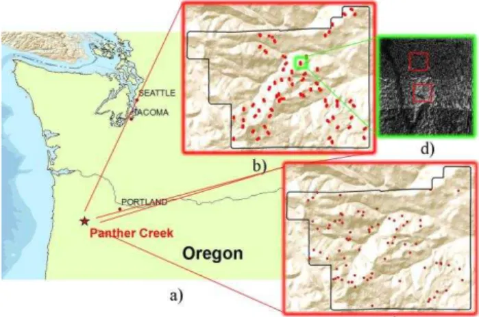
The study area is located in Panther Creek, Oregon (USA) (see Figure 1a). Elevation ranges from 100 to 700 m. The dominant species is Douglas-fir (Pseudotsuga menziesii), being present in more than half of the total forest area, occasionally mixed with other conifers. The height of the trees of the study area is sometimes higher than 60 m, although it is very variable due to timber production in the zone.
Figure 1. Study area: (a) location, (b) paired samples location, (c) field data plot locations, and (d) example of paired sample polygons with different point densities due to overlapping
Full-waveform data were collected in July 15th 2010 by Watershed Sciences, Inc. using a Leica ALS60 sensor on-board a Cessna Caravan 208B. The system acquired data at 105 kHz pulse rate, an average altitude of 900 m above ground level, and a scanning angle of ±15º from nadir. The waveforms were recorded in 256 bins with a temporal sample spacing of 2 ns and beam footprint size of ~0.25 m, what yielded a pulse density of ≥ 8 m-2. The study area was surveyed with opposing flight line side-lap ≥ 50% (≥ 100% total overlap). Aircraft position was recorded with a frequency of 2 Hz by on-board differential GPS unit, altitude was acquired with a frequency of 200 Hz as pitch, roll and yaw from on-board IMU. LiDAR data were provided in LAS 1.3 format. Moreover, the company provided a digital terrain model (DTM) generated from the last return pulses. The accuracy of the DTM was analysed measuring 33 ground control points with GPS Real Time Kinematic (RTK) technique obtaining a RMSE value of 0.19 m.
A total of 64 pairwise samples covering all the study area were located depending on density variations identified (see Figure 1b). Each pair includes a sample measured in a high density area, affected by flight line effect, and another adjacent sample with similar features but with a lower point density and not being affected by the abovementioned effect (see Figure 1d and
2). The area of each sample was 880 m2 similar in size to the field data plots available. Polygon average values of each LiDAR full-waveform metric were extracted so as to study dissimilarities between pairwise samples.
Figure 2. Flight stripe side-lap effect detected in (a) Return Waveform Energy (sum of waveform intensities) metric and (b)
LiDAR point cloud with variable density
In order to estimate structure and canopy fuel load variables, field data were available from 78 circular plots with 16 m radius (see plot distribution in Figure 1c). Plot positions were located with accuracy lower than 0.3 m in horizontal and vertical locations using Trimble R-8 GNSS and Leica TPS 800 total stations. All trees within plots having a diameter at breast height (DBH) greater or equal than 2.5 cm were measured.
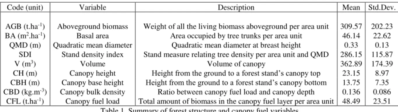
Estimation of forest stand variables were calculated from field data and allometric equations described by Standish et al. (1985) (Hermosilla et al., 2014). These variables were used in regression models as dependent variables (see Table 1).
3. METHODS
3.1 Variable description
Eight LiDAR full-waveform metrics were extracted following those proposed by Duong (2010) and further described by Cao et al. (2014), and used as independent variables in regression models (Crespo-Peremarch et al., 2016): Height of median energy (HOME), Waveform distance (WD), Number of peaks (NP), Roughness of outermost canopy (ROUGH), Height/median ratio (HTMR), Vertical distribution ratio (VDR), Return of waveform energy (RWE) and Front slope angle (FS). Nine forest structure and canopy fuel variables were employed as dependent variables in regression models (see Table 1).
3.2 Data modifications
Two parameters were tested and evaluated in order to minimise the effect due to pulse density changes between flight stripe side-lap areas: voxel size and voxel value assignation.
A correct voxel size is essential. Its dimension is related to LiDAR density and, in case of working with imagery, to the spatial resolution as well (Wang and Glennie, 2015). In our case, initial voxel size was (0.25 x 0.25 x 0.3 m), being 0.25 m the beam footprint size and 0.3 the distance travelled by a pulse in 2 ns, that is the temporal sample spacing. Low density areas are more likely to have empty voxels than high density areas, therefore some LiDAR full-waveform metrics may be affected
Code (unit) Variable Description Mean Std.Dev.
AGB (t.ha-1) Aboveground biomass Weight of all the living biomass aboveground per area unit 309.57 202.23 BA (m2.ha-1) Basal area Area occupied by tree trunks per area unit 46.14 22.62
QMD (m) Quadratic mean diameter Quadratic mean diameter at breast height 0.33 0.13 SDI Stand density index Stand measure relating tree density per area unit and QMD 286.15 115.87
V (m3) Volume Volume of canopy 362.89 174.39
CH (m) Canopy height Height from the ground to a forest stand’s canopy top 23.15 8.97 CBH (m) Canopy base height Height from the ground to a forest stand’s canopy bottom 13.75 7.35 CBD (kg.m-3) Canopy bulk density Ratio between canopy fuel load and canopy depth 0.136 0.086
CFL (t.ha-1) Canopy fuel load Total amount of biomass in the canopy fuel layer per area unit 48.49 23.51 Table 1. Summary of forest structure and canopy fuel variables
as well, having different metrics in adjacent areas with similar features (see Figure 3). In order to reduce this problem, different voxel sizes were tested in the X and Y dimensions: 0.5, 1 and 2 m. Voxel size in the Z-axis was not modified, since it would have reduced the number of bins of the waveform and, subsequently, its accuracy.
Figure 3. Schematic representation of waveform variability related to point density and maximum value within voxels: (a)
higher density and (b) lower density.
The second parameter tested was the criteria to assign the voxel values. Previous studies selected the maximum amplitude of all the waveforms within the voxel (Hermosilla et al., 2014). However, the maximum value increases the probability of having higher voxel values in those areas with higher point densities, biasing the results and increasing the differences. In order to avoid this problem, mean, median, mode, percentiles 90 and 95 of the points that are inside the voxel were tested beside maximum. Combination of both parameters was carried out, testing voxel size modification and criteria to voxel value assignation, thus having 192 different testing sets (8 variables x 4 voxel sizes x 6 value assignations).
3.3 Statistical tests and variable standardisation
Two different statistical tests were employed depending on residual errors distribution and equality of variances (Student’s t-test – Wilcoxon test), to assess statistically significant differences between LiDAR full-waveform metrics measured in low and high density areas. Additionally the difference between paired samples using standardised variables was quantified (see Figure 4).
Figure 4. Flowchart of the overall process followed to assess and quantify dissimilarities between pairwise samples.
Test selection depended on distribution of residual errors and equality of variances hypothesis verifications (see Figure 4). In order to assess if the residual errors follow a normal distribution, being in our case the difference between paired samples measured in flight stripe side-lap and not flight line areas, Shapiro-Wilk W test (Shapiro and Wilk, 1965) was used. F-test (Box, 1953) was employed to assess equality of the variances. For normal distributed and equality of variances cases, a paired Student’s t-test (Gosset, 1908) was employed, which verifies whether the average of differences between paired samples is significantly different from zero (Demšar, 2006). In other cases, Wilcoxon signed-rank test (Wilcoxon, 1945) was used, that compares two samples to assess if dissimilarities between them are significant or not. This test ranks absolute values of differences between paired samples, and compares the ranks for the negative and positive differences separately, being not significantly different when negative and positive ranks are similar (Demšar, 2006).
Student’s t-test or Wilcoxon signed-rank test were employed in the 192 testing samples abovementioned. Test results just assessed whether differences were significant or not, but they were not quantified. Therefore, it was no possible to demonstrate that voxel size and criteria to voxel value assignation improved the results. For this purpose, differences between paired samples in high and low density areas were calculated so as to check if these values decreased (see Figure
4).
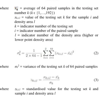
Each LiDAR full-waveform metric has different units, and mean values vary from 0.136 to 361.9 in our study area. In order to compare all the variables, a variable standardisation was applied, using:
(1)
where = average of 64 paired samples in the testing set number k (k ϵ {1,…,192})
xk,i,l= value of the testing set k for the sample i and density area l
k = indicator number of the testing set i = indicator number of the paired sample
l = indicator number of the density area (higher or lower point density area)
(2)
where σk2 = variance of the testing set k of 64 paired samples
(3)
where zk,i,l = standardised value for the testing set k and sample i and density area l
After variable standardisation, absolute value of differences between paired standardised samples was obtained, and afterwards the average of these differences was calculated for each testing variation:
(4)
where Dk = average of the absolute value of differences between paired standardised samples
This average identifies and quantifies the existence of differences in the statistical abovementioned, and it was used to check whether voxel size and voxel value assignation changes decreased variable dissimilarities due to pulse density changes between flight stripe side-lap areas.
3.4 Regression models
Estimation of structure and canopy fuel variables was also affected by pulse density changes, since they were estimated using LiDAR full-waveform metrics. New regression models were generated after modification of the voxel size and the criteria for voxel value assignation in order to evaluate if the flight stripe side-lap effect was corrected (see Figure 4).
LiDAR full-waveform metrics explained in Cao et al. (2014) and modified with the criteria voxel size and voxel value assignation were used as independent variables, while structure and canopy fuel variables calculated according to field data were the dependent variables (see Table 1).
Firstly, a feature selection was carried out using Bayesian Information Criterion (BIC) (Schwarz, 1978) and selecting a maximum of three variables. Then, a linear regression was applied using the selected features and leave-one-out cross-validation. This process was carried out for the initial data as a reference (0.25 m voxel size and assigning the maximum value of all the waveforms within the voxel), and for the testing set that reduced metric differences between paired samples after applying statistical tests and calculating differences of standardised variables. Regression models were evaluated using adjusted coefficient of determination (R2), root-mean-square error (RMSE), normalised root-mean-square (nRMSE), defined as the ratio of RMSE and the range of observed values, and the coefficient of variation (CV), as the RMSE divided by the mean of observed values.
Afterwards, structure and canopy fuel variables were estimated for a small zone (4 km2) of the study area using the two regression models mentioned: the initial one as a reference and the model selected (Figure 4).
4. RESULTS AND DISCUSSION
Table 2 shows statistical results for each testing variation carried out, indicating when differences are statistically significant between paired samples, being our target to achieve a greater number of variables with no statistical dissimilarities.
0.25 m
Max. Mean Median Mode p90 p95
HOME NO NO NO NO NO NO
WD NO NO NO NO NO NO
NP YES YES YES YES YES YES
ROUGH YES YES NO NO YES YES
HTMR NO NO NO NO NO NO
VDR YES YES YES YES YES YES RWE YES YES YES YES YES YES FS YES YES YES YES YES YES
a) 0.5 m
Max. Mean Median Mode p90 p95
HOME NO NO NO NO NO NO
WD NO NO NO NO NO NO
NP YES YES YES YES YES YES
ROUGH NO NO YES YES NO NO
HTMR NO YES YES YES NO NO
VDR YES YES YES YES YES YES RWE YES YES YES YES YES YES FS YES YES YES YES YES YES
b) 1 m
Max. Mean Median Mode p90 p95
HOME NO NO NO YES NO NO
WD NO NO NO NO NO NO
NP YES YES YES YES YES YES ROUGH YES YES YES YES YES YES
HTMR NO YES YES YES YES NO
VDR NO YES YES YES YES YES
RWE YES NO YES YES YES YES
FS YES YES YES YES YES YES c)
2 m
Max. Mean Median Mode p90 p95
HOME NO NO NO NO NO NO
WD NO NO NO NO NO NO
NP YES YES YES YES YES YES ROUGH YES YES YES YES YES YES
HTMR NO NO NO NO NO NO
VDR NO NO NO NO NO NO
RWE YES NO NO YES YES YES
FS YES YES YES YES YES YES d)
Table 2. Statistical test results for each testing set: (a) 0.25 m, (b) 0.5 m, (c) 1 m, and (d) 2 m. “YES” and red-coloured cells
indicate that there was a significant difference at 95% of confidence level, whereas “NO” and green-coloured cells means
that there was not a significant dissimilarity.
As shown in Table 2, HOME and WD are the only variables that are never significantly different, with the exception of HOME in the 1m-mode testing variation. On the contrary, NP and FS paired samples are always significantly different. Other metrics, such as VDR and RWE, become homogeneous when voxel size increases; ROUGH achieves its best result using a voxel size of 0.5 m; and HTMR becomes statistically different for 0.5 and 1 m, and more homogeneous for 0.25 and 2 m.
As observed in Table 2, voxel size parameter generates a higher impact between metrics differences than voxel value assignation criteria. Depending on voxel size, some voxel value assignations generate paired samples more homogeneous.
Analysing the different testing variations carried out and displayed in Table 2, 2m-mean and 2m-median were the testing sets having more variables with no significant differences between high and low density areas (5). This leads to affirm that voxel size modification (from 0.25 m to 2 m) and voxel value assignation change (from maximum to mean or median) reduced significant differences according to statistical tests, except for the variable ROUGH.
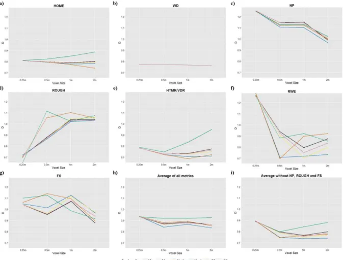
Figure 5 displays, for LiDAR full-waveform metrics, the absolute value averages of differences between standardised paired samples in each testing set, allowing for quantifying and comparing statistical test results.
VDR is displayed together with HTMR in Figure 5. HTMR and VDR graphs are identical, since when differences are calculated for both metrics the same equation is obtained.
In (5) is observed that ΔHTMR = - ΔVDR, and working with absolute value, like in our case, variable differences are identical.
(5)
Figure 5 displays four different global behaviours: WD and NP differences decrease when voxel size increases; HOME, HTMR, VDR and RWE results improve with 0.5 and 1 m voxel size (except mode); FS has not a clear behaviour, increasing and decreasing differences depending on voxel size; and ROUGH clearly increases when voxel size is larger.
For HOME, HTMR and VDR variables, it is observed that the assignation of the median shows slightly lower differences, but the mode increases these dissimilarities between high and low density areas.
In Figure 5h, the differences between voxel size and criteria to voxel value assignations are shown. There is a great improvement between 0.25 m and 0.5 m or 2 m, and dissimilarities increase for 1 m with respect to 0.5 m and 2 m. Regarding voxel value assignation, the mean achieves the best results and the mode the worse.
As observed in Figure 5i, the mean has the lowest differences and the mode the largest differences. Additionally, all the assignations achieve their best results with 1 m, except for mean, median and mode. For the mean assignation, 0.5, 1 and 2 m are similar, being 2m-mean the lowest difference of all the testing sets. Comparing with Figure 5h, all the dissimilarities decrease after deleting those variables (NP, ROUGH and FS) that present the main differences between paired samples.
It can also be observed that all the voxel value assignations have similar behaviour when voxel size is lower. This is due to the fact that when voxels are smaller they have less waveforms crossing inside, therefore these differences are smaller or inexistent if just one point is within the voxel. WD metric is identical for all the voxel value assignations, since this variable is measured from the beginning of the waveform, which is not modified by voxel value assignation changes.
According to Figure 5h and 5i, 2m-mean testing set is the one with the lowest differences between paired samples, which confirms statistical tests. Differences between Table 2 and Figure 5 are due to the fact that statistical tests compare measures of central tendency (mean and median), while the absolute value of paired samples differences quantifies the module of the errors. There are some cases where mean or median of errors are close to zero because negative and positive errors are neutralised, whereas absolute value of paired sample differences show that the difference is not close to zero. In this case, the median value would not be able to detect outliers, because it makes a balance between negative and positive ranking errors, but it does not quantify the differences. This is why statistical tests are complemented by absolute value of paired sample differences.
In the cases where a testing set is significantly different (see Table 2), this is because the differences between paired samples are neutralized and the average is close to zero, but absolute value of paired sample differences have large values (see Figure 5): HOME in 2m-mode; ROUGH in 0.5m-maximum, 0.5m-mean, 0.5m-p90 and 0.5m-p95; HTMR in 2m-mode; VDR in 2m-mode; RWE in 2m-median.
On the contrary, there are some cases where statistical tests show statistically significant differences (see Table 2), whereas absolute value of paired sample differences (see Figure 5) is small. This is because negative and positive differences are not balanced, but the absolute value of these differences is small. This is detected in: ROUGH in 0.25m-maximum, 0.25m-mean,
Figure 5. Graphs displaying the average of differences between standardised paired samples for each LiDAR full-waveform metric: (a) HOME, (b) WD, (c) NP, (d) ROUGH, (e) HTMR/VDR, (f) RWE, (g) FS, (h) average of all metrics differences between standardised paired samples for each testing set, (i) represents the same as h) but without including NP, ROUGH and FS variables
0.25m-p90 and 0.25m-p95; HTMR in 0.5m-mean, 0.5m-median, 0.5m-mode, 1m-mean, 1m-median and 1m-p90; VDR in 0.25-maximum, 0.25-mean, 0.25m-median, 0.25m-mode, 0.25m-p90, 0.25m-p95, mean, median, p90 and 1m-p95; RWE in 0.5m-mean, 0.5m-median and 1m-p90.
Although NP and VDR improvement is not reflected in the statistical tests (see Table 2), Figure 5c and 5e show how the differences between high and low density areas decrease. However, this is not enough to be statistically different.
Comparing the overall results of LiDAR full-waveform metrics in Figure 5, HTMR, VDR, WD and HOME have the lowest differences, while FS and NP have the largest dissimilarities. However, for the selected testing set (2m-mean) RWE has the lower differences and ROUGH the largest.
Statistical tests show a slight improvement (see Table 2), but in Figure 5 can be noticed how voxel size and assignation type modifications produce more homogeneous samples. Even ROUGH variable results, where voxel size modification does not reduce the differences, are improved when assignation type is changed from maximum to median or mode using 0.25 m voxel size (see Figure 5d).
Table 3 shows the results of the different regression models for each estimated variable using initial data as a reference (0.25m-maximum) and the testing variation selected after analysing statistical results and differences between paired samples
(2m-mean).
Table 3 shows that regression models generated with 2m-mean globally improve with respect to the results obtained with 0.25m-maximum, but these differences are small (up to 3%). This can be explained because plots are small compared to flight stripe side-lap areas, and a plot could be completely inside or outside this area, not being the pulse density variations reflected in the results.
Figure 6 shows the estimation of quadratic mean diameter (QMD) variable for a small zone of the study area using (5a) 0.25m-maximum and (5b) 2m-mean data.
QMD was estimated using HOME and HTMR variables for the 2m-mean testing set, which according to Table 2d, Figure 5a and 5e has not significant dissimilarities and absolute value of paired sample differences is low. Contrary to Table 3, in Figure 6b shows that the flight stripe side-lap effect disappears when the variable is estimated for a larger area. Figure 6a is also smoother than Figure 6b, because each pixel of the latter contains less voxels.
5. CONCLUSIONS
Using an appropriate combination of voxel sizes and value assignation method, the flight stripe side-lap effect in LiDAR
Variable Evaluation parameter 0.25m-max. 2m-mean
AGB
R2 0.85 0.84
RMSE (t.ha-1) 77.47 80.42
nRMSE 0.09 0.09
CV 0.25 0.26
BA
R2 0.74 0.74
RMSE (m2.ha-1) 11.36 11.23
nRMSE 0.11 0.11
CV 0.25 0.24
QMD
R2 0.78 0.78
RMSE (m) 0.06 0.06
nRMSE 0.09 0.10
CV 0.18 0.19
SDI
R2 0.66 0.68
RMSE 67.07 63.96
nRMSE 0.12 0.11
CV 0.23 0.22
V
R2 0.72 0.73
RMSE (m3) 89.66 89.38
nRMSE 0.11 0.11
CV 0.25 0.25
CH
R2 0.65 0.68
RMSE (m) 5.16 4.95
nRMSE 0.12 0.11
CV 0.22 0.21
CBH
R2 0.70 0.72
RMSE (m) 3.89 3.81
nRMSE 0.10 0.10
CV 0.28 0.28
CBD
R2 0.65 0.66
RMSE (kg.m-3) 0.05 0.05
nRMSE 0.13 0.13
CV 0.36 0.36
CFL
R2 0.76 0.74
RMSE (t.ha-1) 11.30 11.81
nRMSE 0.11 0.11
CV 0.23 0.24
Table 3. Results of different regression models for each estimated variable
full-waveform metrics can be significantly reduced. When using LiDAR full-waveform data with point density variability and similar characteristics than the one used in the tests, a voxel size of 2 m and the assignation of the mean amplitude value of all the waveforms within the voxel is recommended to reduce this effect in metric values. There are relevant differences of this effect depending on which metrics are considered. In the test we developed, some full-waveform metrics highly affected by point density variations are: NP, ROUGH and FS. After removing these metrics, differences between different point density areas were reduced using the assignation of the mean amplitude value of all the waveforms within the voxel and a voxel size of 0.5, 1 or 2 m. After voxel size and assignation value modification, flight line side-lap effect is reduced in the forest structure and canopy fuel variable maps.
In addition to voxel size and criteria to voxel value assignation, other data treatments can be carried out in further work, such as point filtering techniques to equalise densities in all the area. These techniques could be made by analysing point density along the study area and then selectively reducing it until obtaining an homogeneous distribution, or using the flight trajectory information to detect flight stripe side-lap areas and
then removing LiDAR points in order to equalise densities.
a)
b)
Figure 6. Estimation of quadratic mean diameter (QMD) for a small zone of the study area using (a) 0.25m-maximum (the effect is evident in some flight lines), and (b) 2m-mean data.
ACKNOWLEDGEMENTS
This research has been funded by the Spanish Ministerio de Economía y Competitividad and FEDER, in the framework of the project CGL2013-46387-C2-1-R.
The authors also thank the Bureau of Land Management and the Panther Creek Remote Sensing and Research Cooperative Program for the data provided for this research.
REFERENCES
Box, G.E.P., 1953. Non-normality and tests on variances. Biometrika, 40(3/4), pp. 318-335.
Buddenbaum, H., Seeling, S., Hill, J., 2012. Fusion of full-waveform lidar and imaging spectroscopy remote sensing data for the characterization of forest stands. International Journal of Remote Sensing, 34(13), pp. 4511-4524.
Cao, L., Coops, N.C., Hermosilla, T., Innes, J., Dai, J., She, G., 2014. Using small-footprint discrete and full-waveform airborne LiDAR metrics to estimate total biomass and biomass components in subtropical forests. Remote Sensing, 6, pp. 7110-7135.
Crespo-Peremarch, P., Ruiz, L.A., Balaguer-Beser, A., Estornell, J., 2015. Análisis temporal de la estructura forestal mediante métricas derivadas de LiDAR full-waveform. In:
Actas XVI Congreso de la Asociación Española de Teledetección, Sevilla, Spain, pp. 387-390.
Crespo-Peremarch, P., Ruiz, L.A., Balaguer-Beser, A., 2016. A comparative study of regression methods to predict forest structure and canopy fuel variable from LiDAR full-waveform data. Revista de Teledetección, 45, pp. 27-40.
Demšar, J., 2006. Statistical comparisons of classifiers over multiple data sets. Journal of Machine Learning Research, 7, pp. 1-30.
Duong, H.V., 2010. Processing and application of ICESat large footprint full waveform laser range data. Ph.D. Thesis, Delft University of Technology, Netherlands.
Erdody, T.L., Moskal, L.M., 2010. Fusion of LiDAR imagery for estimating forest canopy fuels. Remote Sensing of Environment, 114(4), pp. 725-737.
Franco-Lopez, H., Ek, A.R., Bauer, M.E., 2001. Estimation and mapping of forest stand density, volume, and cover type using the k-nearest neighbors method. Remote Sensing of Environment, 77(3), pp. 251-274.
Gosset, W.S., 1908. The probable error of a mean. Biometrika, 6(1), pp. 1-25.
Hermosilla, T., Ruiz, L.A., Kazakova, A.N., Coops, N.C., Moskal, M., 2014. Estimation of forest structure and canopy fuel parameters from small-footprint full-waveform LiDAR data. International Journal of Wildland Fire, 23(2), pp. 224-233.
Lefsky, M.A., Cohen, W.B., Acker, S.A., Parker, G.G., Spies, T.A., Harding, D., 1999. Lidar remote sensing of the canopy structure and biophysical properties of Douglas-fir western hemlock forests. Remote Sensing of Environment, 70(3), pp. 339-361.
Means, J.E., Steven, A.A., Brandon, J.F., Renslow, M., Emerson, K., Hendrix, C.J., 2000. Predicting forest stand characteristics with airborne scanning lidar. Photogrammetric Engineering & Remote Sensing, 66(11), 1367-1371.
Naesset, E., 2002. Predicting forest stand characteristics with airborne scanning laser using a practical two-stage procedure and field data. Remote Sensing of Environment, 80(1), pp. 88-99.
Schwarz, G., 1978. Estimating the dimension of a model. The annals of statistics, 6(2), pp. 461-464.
Shapiro, S.S., Wilk, M.B., 1965. An analysis of variance test for normality (complete samples). Biometrika, 52(3/4), pp. 591-611.
Standish, J.T., Manning, G.H., Demaershalk, J.P., 1985. Development of biomass equations for British Columbia tree species. Canadian Forestry Service, Pacific Forest Research Center, Information Report BC-X-264, Victoria, BC, Canada.
Temesgen, H., Strunk, J., Andersen, H-E., Flewelling, J., 2015. Evaluating different models to predict biomass increment from multi-temporal lidar sampling and remeasured field inventory data in South-Central Alaska. Mathematical and Computational Forestry & Natural-Resource Sciences, 7(2), pp. 66-80.
Wang, H., Glennie, C., Prasad, S., 2013. Voxelization of full waveform lidar data for fusion with hyperspectral imagery. In: Proceedings of the IEEE International Geoscience and Remote Sensing Symposium, pp. 3407-3410.
Wang, H., Glennie, C., 2015. Fusion of waveform LiDAR data and hyperspectral imagery for land cover classification. ISPRS Journal of Photogrammetry and Remote Sensing, 108, pp. 1-11.
Wilcoxon, F., 1945. Individual comparisons by ranking methods. Biometrics Bulletin, 1(6), pp. 80-83.
Zimble, D.A., Evans, D.L., Carlson, G.C., Parker, R.C., Grado, S.C., Gerard, P.D., 2003. Characterizing vertical forest structure using small-footprint airborne LiDAR.