I
NCOME AND
B
ARGAINING
E
FFECTS ON
E
DUCATION AND
H
EALTH
V
LADIMIRP
ONCZEKOutubro
de 2009
T
Te
ex
xt
to
os
s
p
p
a
a
ra
r
a
D
TEXTO PARA DISCUSSÃO 216 • OUTUBRO DE 2009 • 1
Os artigos dos Textos para Discussão da Escola de Economia de São Paulo da Fundação Getulio Vargas são de inteira responsabilidade dos autores e não refletem necessariamente a opinião da
FGV-EESP. É permitida a reprodução total ou parcial dos artigos, desde que creditada a fonte.
Income and Bargaining Effects on Education and Health
∗Vladimir Ponczek†
Sao Paulo School of Economics - Getulio Vargas Foundation.
May 31, 2007
Abstract
In this paper, we examine the impacts of the reform in the rural pension system in Brazil in 1991 on schooling and health indicators. In addition, we use the reform to investigate the validity of the unitary model of household allocation by testing if there were uneven impacts on those indicators depending on the gender of the recipient. The main conclusion of the paper is that the reform had significantly positive effects on the outcomes of interest, especially on those co-residing with a male pensioner, indicating that the unitary model is not a well-specified framework to understand family allocation decisions. The highest impacts were on school attendance for boys, literacy for girls and illness for middle-age people. We explore a collective model as defined by Chiappori (1992) as one possible alternative representation for the decision-making process of the poor rural Brazilian families. In the cooperative Nash equilibrium, the reform effects can be divided into two pieces: a direct income effect and bargaining power effect. The data support the existence of these two different effects. [JEL=O15, I12, I28]
∗I would like to thank Anne Case for encouragement and extraordinary guidance. I also thank Fernando Botelho, Carlos
Bozzoli, Scott Fulford, Chris Paxson, Nisreen Salti, Luke Williard, and participants of the development lunch seminar at Princeton University for comments and suggestions. All remaining mistakes are mine.
1
Introduction
In the past decades, the economic literature has shown evidence that the household cannot be characterized as a unit with individuals sharing the same preferences or pooling their resources. Within the family unit different individuals may have different concerns about how to spend their total family income and the decision-making process of the resource allocation may be affected by the difference in preferences. This paper intends to take advantage of variation in social security system rules in Brazil to estimate the impact of a change in family income on socio-economic outcomes and uses that to investigate the decision-making process of the affected families.
Fully understanding the decision process is important in order to make better and more efficient transfer policies. Using the unitary model of the household as a guideline for policy prescriptions may be misleading, since the effect of public transfers may differ depending on the identity of the income recipient. Therefore, targeting transfers to the household may not result in the desired consequences, given that transfers directed to the head of the family, to the spouse or to elderly people may have different impacts over the family. For example, if the receiver of the transfer were an elderly person, there could be a larger fraction of the transfer allocated to health care. In the same way, if the beneficiary were the mother instead of the father, the income augment might cause a reduction on her labor supply, since she might now want to allocate more of her time raising the children. Hence, an increase in the family income may have uneven impacts on different members of the household depending on the characteristics of the transfer recipient.
In many developing countries, the pension system is the most important source of public transfers to poor families. Therefore, a major change in the rules of the social security system in a continental country is an excellent opportunity to understand how income is allocated within household members. We will take advantage of the Brazilian social security reform that occurred in 1991 to measure the extent to which the impacts of an unanticipated increase in pension income depend on the characteristics of the pensioner.
the social security system may cause a massive change in intra-household allocations. For instance, if female pensioners are concerned more about children education, a change in the pension rules that allows spouses to also be a recipient may cause an important boost in schooling for children living with an elderly female. In this case, the impact would be even higher than one caused by a male beneficiary. Thus, estimating uneven impacts of the reform on different family members creates a possibility to better understand how intra-household allocations are designed. In this research, we plan to concentrate the analysis of the impact of changes in the pension system rules on two different outcomes: education and health. Both issues are important to the design of policies with the goal of enhancing the quality of life of poor families and reducing inequality in developing countries.
Since Becker published his seminal works1 on family behavior, there has been a great number of theoretical and applied research interested in the analysis of intra-household allocation. Theneoclassical traditional view, the unitary model of intra-household allocation, assumes that the family behaves as a single agent. An important implication of this model is that the expenditure on family’s public good (e.g. children’s schooling, health, etc) depends only on the total family income and redistribution of income among family members has no effect on the provision of the public good. The literature defines this property as a “neutrality” result.2 As discussed by Ermisch (2003), the “neutrality” condition can be also obtained even in a framework where individuals within a family have different preferences and are allowed to make distinct decisions about consumption. In this case, we have to assume that individuals do not cooperate in making decisions, i.e., each member chooses his contribution to the public good to maximize his own welfare, taking the contribution of the other members as given and also that preferences are convex. In the case ofinterior solutions, where each individual contributes a non-zero amount of public good and care only about the private consumption and the total amount of public good, the “neutrality” condition holds. Another characteristic of the non-cooperative outcome is the Pareto inefficiency.
On the other hand, in a cooperative Nash equilibrium, adults maximize their utility func-tion constrained by given levels of utility achieved by the other adult members. Therefore, the equilibrium should be Pareto-Efficient, in the sense that in the equilibrium allocation of public and private goods, no adult can be better off without making at least one of the others worse off. This is called the “collective model” by Chiappori (1992). In this situation,
1
See Becker (1964), Becker (1974) and Becker (1981).
2
for types of preferences usually assumed in economic analysis, a redistribution of resources among the family members will potentially affect the amount of public good, and it will increase or decrease depending on the preferences of the receiving adult.3 The result works as if there was an income sharing rule, i.e., each member has a share of the total family income and chooses his contribution to the public good based on his own preferences and the share of income. Chiappori (1992) interprets the share as a reflection of the bargaining power within the family. Therefore, an increase in a member’s income will generate two separate effects: (i) a direct income effect that increases the provision of the public good as long as it is a normal good; (ii) a bargaining effect which reinforces the income effect if the member who received the extra income has stronger preferences in favor of the public good compared to the other members.
The empirical investigation about the unitary model of intra-household allocation is a recurrent topic in the literature. A classic study by Thomas (1990) which also uses Brazilian data, tests whether the mother’s unearned income has a different impact on family health than the father’s. He finds differential effects for child survival, and thus rejects the neo-classical model. He also observes that mothers favor their daughters, and fathers their sons in terms of nutritional intakes. Duflo (2003) uses the South African social pension program to study whether the impact of cash transfer on child nutritional status is affected by the gender of the recipient. The author claims that pensions received by women have an impact on the anthropometrics status (height) of girls but little effect on boys. However, she could not find a similar effect for pensions received by men. Emerson and Souza (2007) study the existence of uneven impacts of parent’s socio-economic characteristics on school attendance and child labor for boys and girls. Their results show that the father’s characteristics such as years of schooling, non-labor income, and the age he first began working have a greater impact on sons than on daughters while mother’s characteristics have are greater effect on daughters. Moreover, the authors find that both non-labor income of mothers and fathers affect the son’s schooling attendance more than they affect daughter’s attendance.
Delgado (1997) and Delgado (1999) descriptively report the impacts of the reform on socio-economic indicators such as poverty, personal and regional income distribution and find a significant reduction of poverty and income redistribution for families affected by the reform. Carvalho (2000) and Carvalho (2001) also focus on the 1991 Brazilian reform. He
3
studies the impact of the income variation caused by the social security changes on schooling decisions, child labor, retirement decisions and labor market responses. In the first paper, the author finds a reduction in child labor for both girls and boys and positive impact on schooling enrollment for both genders, but does not focus on intra-household allocation or bargaining power. In the second paper, he also observes a reduction in the retirement age among those affected by the reform.
In summary, the literature from developing countries has used social security reforms to investigate whether pension income is associated with better outcomes for individuals who live with pensioners and to explore whether characteristics of pensioners affect the allocation of resources in the household. The restructuring in the Brazilian social security system presents itself as a valuable opportunity to understand the individual and family responses to unanticipated income shocks. This study intends to explore the exogenous variation in income caused by the rural pension system reform in Brazil to estimate the impact on the cited social outcomes (education and health). Our primary objective in this paper is to test whether an extra amount of family income coming from the social security benefits creates uneven impacts on different members depending on the gender of the beneficiary.
The empirical strategy consists of estimating whether the variation in income driven by the social security reform generated a different impact on the demand for the public goods (schooling and health) depending on the gender of the eligible member, and also whether the pension income was spent like any other non-pension income or not. If the “neutrality” property holds, it is expected that the pension income is spent like income from any other source and also that the gender of the pensioner will not be significantly related to the provision of the public good.
This paper is organized as follows: Section 2 discusses about the dataset used in this paper. Section 3 explains the details of the reform. Identification strategies are discussed in section 4. The results are analyzed in section 5 and show a positive impact on schooling and health status for boys living with male pensioners suggesting that the unitary model is not valid. Section 6 concludes.
2
Data
The data used in this research come from thePesquisa Nacional por Amostra de Domic´ılios
1/500 of the Brazilian population (about 100,000 households) and is designed to produce a picture of the social-economic conditions of the Brazilian population. It covers all urban and almost all rural areas, except the Amazon region. It has been conducted on a regular basis since 1981 byIBGE (the Brazilian Census Bureau) except in years in which census data was collected (1991 and 2000) and in 1994 when there was a budgetary crisis. PNAD contains also extensive data on personal and household information. For each person, information about age, schooling attendance, literacy, migration, labor participation, retirement and income sources (including amounts) is available. Moreover, periodically questions about some other special topics (the “Supplements”) are included in the survey. For instance, in the 1970’s, questions about migration were included; in the 1980’s the special topics were heath education, labor market and social security; in the 1990’s, migration, fertility and child labor. To study the schooling outcomes (literacy and attendance), we will use the 1988, 1989 and 1990 PNAD’s for years before the reform took place (1991), and the 1992, 1993 and 1995 surveys for years after the reform. We will analyze the impact on children between 6 and 18 years old who live in rural areas. In the case of health indicators, we will use the PNAD supplements’ information collected prior the reform (1986) and from one collected after the reform (1988). Two indicators will be evaluated: reported illness and the search for any health care service in the past two weeks prior to the interview. We study the effects of the reform on those two health indicators for different subgroups (everyone, children - between 0 and 14 years old) and middle-age people - men between 40 and 55; and women between 40 and 50 years old).
3
The Reform
In October of 1988, the new Brazilian Constitution was promulgated. The Constitution established many changes in the principles of the entire social security system. In addition, it also determined that the Congress should approve Ordinary Laws, which should implement all changes. The main guiding principles stipulated by the Constitution were: extension of old-age benefits to anyone who was not a household head; no benefit should be smaller than one minimum wage; reduction in the minimum age of old-age eligibility; length-of-service eligibility to rural workers.4 The Congress passed the Ordinary Laws 5 on July 24 of 1991
4
Beltraoet al.(2003) and Delgado (1997) have more details about the constitutional new rules concerning the rural pension system.
5
Laws # 8212 and 8213, available at
and the reforms went into effect. The new main rules sanctioned by the law were:
• New minimum age eligibility equal to 60 for men and 55 for women compared to 65 years for both men and women before the reform.
• Anyone who reached the minimum age requirement could be eligible in the household.
• The minimum benefit was increased to 100% of the minimum wage.
• The value of the benefit is calculated based on previous earnings against a flat benefit of 50% of minimum wage before the reform.
• Length-of-service pension available after 30 years of services for men and 25 years for women. The value of the benefit is also calculated based on previous earnings.
Beyond minimum age, eligibility to a rural pension requires from the worker proof of residence in a rural area and engagement in one of the rural activities defined by the law (farmers, fishers, miners, loggers, etc.) for at least 60 months prior to the application. Proving previous engagement in a rural activity was extremely easy, since many documents were accepted as sufficient proof, such as individual labor contracts, tenancy contracts and sharecropping agreement, among others.
Although the law stipulated an earning-based benefit, the great majority of the rural pensioners received the minimum wage at least until 1997 because almost all rural workers did not keep a documented record of previous earnings. For instance, the average rural benefit paid in 1997 was around R$ 121, while the minimum wage was R$ 120. For the same reason, the proportion of length-of-service retirees in the rural system is insignificant, less than 0.1% of the total number of pensioners.6 Therefore, we do not worry about any kind of endogeneity caused by differences in the value of the benefit or in the age of retirement.
The increase in the minimum benefit for the current pensioners was instantaneous. The income of those who were pensioners in the old system doubled right after July of 1991. However, for those who are now eligible or decided to apply after the change in the rules, the entire process of registration took several months due to administrative delays. Therefore, for the entire group of people who became eligible after the reform, the impact was not automatic. Beside, since the worker should apply to be registered in the system, concerns about selectivity bias, especially about the timing of the reform impacts, arise. Probably
http://www010.dataprev.gov.br/sislex/paginas/42/1991/8213.htm .
6
many newly eligible workers in a first moment ignored the new rules of the system and it is possible that unobservables correlated to the ignorance of the new rules are also correlated with some outcome of interest. That is one of the reasons why we use datasets until 1995 in order to let the take-up process for the newly eligible complete. In our dataset, the proportion of pensioners among the newly eligible before the reform was around 15%7 and increases to 50% before stabilizing after 1995.
4
Identification Strategies
Consistently estimating the effect of income variations on different family members is not a simple task. Using disparity of income across families from a single cross-section may intro-duce many identification problems in the regressions. A family’s unobserved characteristics might be correlated with family’s income and also with investment in schooling and health. This situation could lead to several misinterpretations of the data. Based on the results of such simple regressions, one could argue, for example, that an extra amount income would imply an increase on schooling attendance, when, in reality, it is the intellectual level of the parents, which is correlated with the family income, that drives the decision about the child schooling. An exogenous source of income variation is a sine qua non condition for having consistent and reliable results. Hence, the modification in the Brazilian social secu-rity system in 1991 is an excellent source of income variation to be explored, since it is not correlated with any family unobserved characteristics.
However, using total income that comes from the benefits or even a direct indicator if the family has a person that is a pensioner is also problematic. The value received from the pension (when it is not the minimum value) is derived from the past labor earnings and could possibly also be correlated with unobservable characteristics. Directly including a dummy variable indicating if the person is a pensioner might also generate inconsistent results, since the decision to apply (and when to apply) to the benefit could potentially be endogenous. For instance, rich people might not be willing to go to a post office and stay in the line in order to apply for the pension, since their extra income utility could not compensate the burden of applying to the pension. In this case, a selectivity bias problem could arise. Therefore, we will pursue a intent-to-treat approach, in which actual treatment is replaced
7
by eligibility in order to avoid the selectivity problem.8
Moreover, the use of variation across households in social security income to identify the impact of earnings on social outcomes requires adequate control of the effects of living with an elderly person unrelated to their social security revenue. Families who co-reside with an elderly person may differ from other families for several reasons. Elderly people may have different preferences over the importance of children education compared to the other family members, or concern more about their own health, or, in general, the presence of an elderly person may be correlated with other unobserved characteristics that are also correlated with the outcomes of interest. Therefore, from one single cross-section, it is impossible to disentangle the direct income effect of coming from the old-age pension from the impacts of living with an elderly person. An exogenous reform in social security, however, permits the separation of theses effects.
Nevertheless, the comparison between the cross-sectional patterns of outcomes before and after the reform would identify the effect of the changes in social security income only in the absence of any ongoing trend. In the presence of such trend a before and after
estimator would be upward or downward biased depending whether the trend is positive or negative sloped. In order to control for the time trend effect, we will use a difference-in-difference approach. The difference-in-difference estimator will be consistent as long as the time variation on the outcome of interest would be the same for both treated and control group in the absence of the treatment, i.e., only if both groups have the same time trend. If the control group has a different time pattern from the treated, the difference-in-difference
estimator will be biased. Suppose Yit,0 and Yit,1 are, respectively, the outcomes for the non-treated and non-treated individual iat time t and they are modeled by the following equations:
Yit,0 =βi,0 +δt,0+ǫit
Yit,1 =βi,1+δt,1+α+ǫit.
whereβi, . are the fixed effects,δt,. are the time effects andα indicates the true effect of the
treatment. Let t =b, a ((b)efore and (a)fter the treatment). For simplicity, we will assume thatδb,1 =δb,0 = 0. Thedifference-in-differenceestimator will only be unbiased ifδa,1 =δa,0,
8
i.e., if both treated and control groups have the same time pattern.
E[αDD] =E[Yia,1−Yib,1]−E[Yia,0−Yib,0]
=α+δa,1−δa,0 =α if δa,1 =δa,0.
Assuming now
δe=1
a,. =δ e=0
a,. + ∆
e. (1)
wheree= 1 indicates if the individual has an elderly member in her family. More specifically, we are assuming that the potential difference in the time trend of thetreatment and control group (∆e) does not come only from the treatment per se, but also from the presence of
an elderly person in the family. An unobservable shock could have affected only families with an elderly member in the same moment of the pension reform. Therefore, in order to obtain an unbiased estimator of the true treatment effect, we need a control group that has an elderly member (e= 1), but was not affected by the reform.
We plan to use families with an almost-eligible person – man between 55 years and 60 years old and/or women between 50 years and 55 years old– as the control group9 in order to disentangle the true treatment effect from the specific elderly trend effect.
Furthermore, the reform is also an extraordinary opportunity to check whether the “neu-trality” property characterizes the intra-household allocation process. Testing the validity of the unitary model without an exogenous income variation may also lead to erroneous conclusions. Most studies in the literature use only the variation across families of unearned income in the hands of different member (for example mothers and fathers) to identify the allocation process within households. They usually regress the children outcomes (health, schooling, anthropometrics, nutrient intakes, etc) on parent’s unearned income. By compar-ing the coefficient of each parent income, those studies gauge the consistency of the unitary model. However, since the difference between unearned incomes of distinct members in the family is not likely to be orthogonal to unobserved characteristics in the family that also affect the outcome of interest, the conclusion based on those estimated coefficients may be invalid. For instance, suppose families that depend more on unearned income care less (both fathers and mothers) about education. In addition, it is possible that the fact that they need more this extra money induces the member of the family who works to also search for these alternative resources. In this case, the difference in unearned income between the working
9
and non-working member of the family would be higher for such families and could lead to a spurious correlation with the outcome of interest. Since the income variation caused by the reform was out of the family’s control and therefore orthogonal to any unobserved characteristic that could be correlated to the provision of the public good, we will test the validity of the unitary model by examining if the reform had uneven impacts on the outcome of interest conditioning on the gender of the eligible person.
The benchmark regression is the following:
E
Y |Tm,f, Cm,fP ost, W
=β0+β1mTm+β
f
1Tf +β2mCm+β
f
2Cf +β3P ost +βm
4 Tm×P ost+β
f
4Tf ×P ost+β5mCm×P ost+β
f
5Cf ×P ost+W γ (2)
whereY is the outcome of interest (explicitly, schooling and health indicators);Tj (for both
j = (m)aleor (f)emale) is a binary variable which is 1 if individual’s family has the presence of at least one eligible person in the new system rules [(Tm) man 60 years or older or (Tf)
woman 55 years or older], i.e., the “treated” group; Cm,f indicates whether the individual
co-resides with at least one male (Cm) or female (Cf) almost-eligible person, i.e., if she is
part of the control group; W is a vector of household and personal characteristics such as age, age squared10, education attainment of the head of household, head’s gender, age and race, number of family members and number of children in family;Post is a dummy denoting post-reform years (after 1991). Tm, Tf, Cm and Cf also enter in the equation interacted
with Post.
With this specification and assuming a linear probability model, β4j (the coefficients of the interaction terms between Tj and Post) will be the difference-in-difference estimators
of the treated against the reference group, which is, in this case, everyone who resides in the rural areas and does not co-reside with an eligible or an almost-eligible person. β4j is consistent as long as ∆e = 0 in equation (1), i.e., bothtreated andreference groups have the
same time trend.
Comparing β4j with β5j allows us to check if β4j are indeed capturing the reform effect driven by the increase in benefits11 or if it is just reveling an elderly presence trend effect.
β4j−β5j is thedifference-in-difference estimator when the comparison is thecontrol group. In this case, bothtreated andcontrolgroups have an elderly member in their family. Therefore,
10
We also tried a specification including dummies for each year of birth in order to capture any cohort effect. The results were qualitatively very similar to those presented here and are available upon request.
11
Actually, in this specification,βj4 is also capturing the effect of the reduction in age eligibility. Below, we will disentangle
even if there is a specific time trend related to the presence of an elderly person,β4j−β5j will consistently estimate the true treatment effect.
Finally, we analyze the validity of the “neutrality” property by testing if βm
4 = β
f
4. Assuming that the direct income impact of the reform was uniform across families with male and female pensioners, difference in the effects on the provision of the public good must be caused by changes in the bargaining power within the household. In other words, if bargaining power has an important role on the allocation decisions, extra income given to men should impact the outcomes of interest differently than income given to women, therefore,
βm
4 6=β
f
4, violating the “neutrality” property and consequently rules out the unitary model as a good specification of the allocation process.
New × old eligibility
Since the decision about applying to the benefit is potentially endogenous, the results based on specification (2) have to be carefully interpreted. As explained in section (3), the reduction in the age eligibility does not guarantee an extra amount of income for families with a newly eligible person right after the reform in the system. Depending on how important the extra income is for the eligible member and her family, the decision of whether and when to apply to the benefit could be different from family to family. And if the source of this “application” heterogeneity was correlated to the outcome of interest, the result estimated would have to be understood differently than if it was not the case. Each β4j in equation 2 captures the average impact of the reform on the entire group of potentially “treated” families.
Moreover, even disregarding the possible heterogeneity problem exposed above, work with just one treatment effect could create another problem, since the impact of the reform on families with a newly eligible was different on those with an old eligible member. More specifically, for those families that have a newly eligible member who now receives the mini-mum benefit, the amount of benefit received was zero before and increased to one minimini-mum wage after the reform. On the other hand, for those who were already beneficiaries, the reform impact was half as much as on the first group. Therefore, again, β4j would capture an “average” effect that could underestimate or overestimate the true impact on each one of those two treatment groups.
in eligibility age we estimate the following:
E
Y |Tkj, P ost, W
=β0+
X
j=m,f " 2
X
k=1
β1j,kTkj
+β2jCj #
+
β3P ost+
X
j=m,f " 2
X
k=1
β4j,kTkjP ost
+β5jCjP ost
#
+W.γ (3)
where Tij′s are: (k = 1) the presence of an individual eligible in the old system rules – 65 years or older person – this term captures the impact of the increase in the minimum benefits values from 50% of the minimum wage to 100% of it.; (k= 2) the presence of a newly eligible individual in the new system rules (between 60 years and 65 years old for men or between 55 years and 65 years old for women) this term also captures the effect of reduction in the age requirement.
In this case, β4j,k=1 and β4j,k=2 will be, respectively, thedifference-in-difference estimators of the treated group 1 and 2 against the reference group. Again, testing β4j,k=1 = β5j and
β4j,k=2 =β5j allows us to check if the effect is coming from the reform or a specific characteristic of families with elderly people.
Again, testing if βm
4,k=1 =β
f
4,k=1 andβ4m,k=2 =β
f
4,k=2 indicates the unitary model validity.
5
Results
Impacts on Income
Before attempting to measure any effect of the changes of the pension system on social-economic outcomes, it is important to be sure that the social security reform has an impact on families’ total income in rural areas.
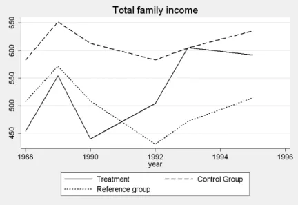
Graph 1 illustrates the variation over time of the total family income12 of the “treated”,
control andreference groups in rural areas. As expected, there was a big jump in the family income with the presence of eligible people after 1990. In 1988, the average family income of that group was R$ 453, lower than the control group’s (R$ 582) and all other families’ income (R$ 507). There was a uniform increase for all groups in 1989 due to the country economic growth and decrease in 1990 after a big economic recession13. In 1992 (after the
12
in September 2002 Reais (R$).
13
reform), the “treated” group experiences a considerable growth in family income. On the other hand, both the control group and all rural families had their income diminished. From 1993 to 1995, Brazil has grew on average 5% per year and that growth is exhibited in the graph: all groups presented significant increase (around 15%) in total family income during the period. From 1988 to 1995, the“treated” group experienced a total family income growth of 30.4% in real terms, while the income of thecontrol group grew only 9.0% and just 1.3% for all other rural families.
In graph 2, the “treated” group is broken into two different groups, depending on the gender of the eligible person. Both Tm and Tf groups’ incomes have very similar path
throughout the period. It is an indicative that uneven impacts of the reform for families with a man or a woman pensioner cannot be credited only to differences in the family income variation. It is more likely that such discrepancies have arisen due to divergences in preferences of male and female recipients.14
As mentioned in section 3, the reform consisted in many different changes in the law. With the dataset available, we were able to disentangle the impacts of two sets of “treatments”: (1) the effect of the increase in the minimum benefit (from half to one minimum wage) and (2) the reduction in the age requirement in order to become eligible (from 65 to 60 years for men and from 65 to 55 for women).
Graph 3 shows the variation of the total family income of both“treated” groups. Clearly, the impact of the minimum benefit increase starts right after the reform in 1992. The rise in the total family income of the “old eligible” group was 30.2% in the first year after the reform, while the impact on family income of the new age eligibility rule was only sufficient to offset the significant recession happened in the country in that period – the total family income of that group was practically stable from 1990 to 1992. From 1992 to 1995, both
“treated” groups presented an increase in the family income. However, in this period the growth in “newly eligible” group was much more significant than the “old eligible” one. The former has increased 30.6% and the latter only 6% in the period. The control and reference
groups experienced an increase of 17.2% and 16.2%, respectively.
The timing of family income boost for the “old eligible” group illustrates the impact of the increase in the minimum benefit value. Since the change in benefit was automatic for everyone already registered in the social security system, the effect was immediate. On the
14
other hand, “newly eligible” individuals had first to register in system before receiving the benefit. Disinformation, administrative delays, transportation costs to the near post office could explain the postponement of the increase in the family income.
From 1988 to 1995, the total increases in the family income were 33.2% for the “old eligible” group; 18.3% for the “newly eligible”; 4.9% for the control group and a decrease of 1.2% for the entire rural sector.
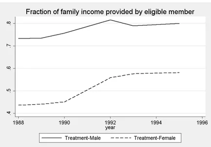
Graph 4 shows that the participation of the eligible person’s income in the total family income has also increased in the period, and graph 5 illustrates that this increase has hap-pened for both male and female recipients, but was more acute for women, since now the system allows spouses to also be pensioners.
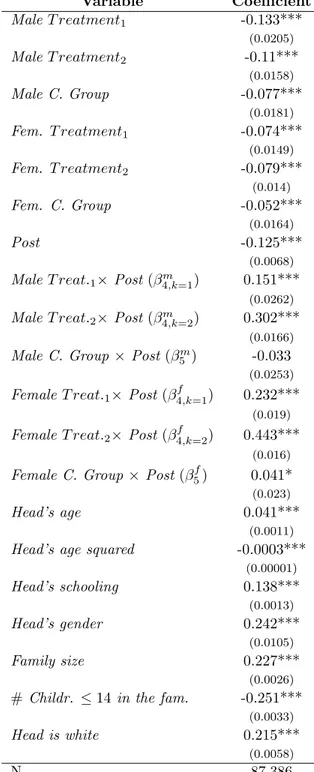
Table 3 shows the results of an OLS regression of model (3) where the dependent variable is the total family income in logs. All control variable coefficients are statistically significant and have the expected sign. The total family income is higher if the head is older (with concavity), more educated, male and white; families with more children also tend to have lower income. It is also worthy noticing that all “treated” are poorer compared to the reference group, indicating that the reform mostly impacted families in the bottom of the income distribution. Looking now at thedifference-in-difference coefficients, the results corroborate the evidence found in the graphs above. The “treated” families have experienced a significant growth in their income after the reform. Allβ4j,i are strongly significantly different from zero and from
their respective counterpart in the control group (β5j). Moreover, the coefficients of the “old eligible” groups (for both male and female pensioners) (β4j,k=2) are statistically significantly higher than the “newly eligible” ones (β4j,k=1). Once more, this could be an illustration of the new registration delays which occurred after the reduction in the eligibility rule. As expected both β4f,k=1 and β4f,k=2 are significantly bigger than βm
4,k=1 and β4m,k=2, indicating a stronger effect on income from the presence of an eligible females compared to the presence of an eligible male. This was due to the new rules concerning the benefits of spouses.
Impacts on Schooling and Health
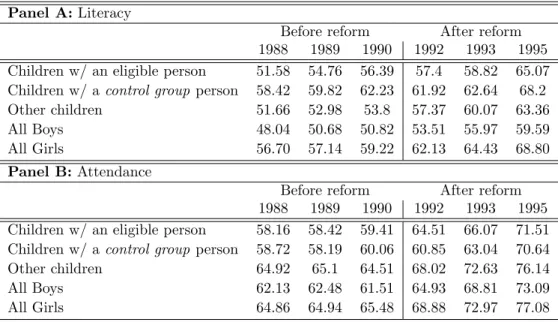
Table (1 shows the evolution of the literacy and attendance and dispicts the improvement of these schooling indicators in Brazil during the period for all groups of families. It illustrates the fact that Brazil has been considerably improving its educational performance, especially in the elementary level of schooling, since the beginning of the last decade.
of schooling) should be freely provided by the municipalities and secondary level (9 to 11 years of schooling) by the states. Although it was possible for almost all children to find a public school within the state, transportation, uniform and other supplies costs impeded the access of a considerable part of the children population. Moreover, since child labor was not a rare phenomenon in rural Brazil, the opportunity cost of the forgone income was also significant. Threfore, we believe that the social security reform which had a significant impact on the families’ budget constraints is also behind the progress of those indicators for the treated families. The increase of the schooling standards in Brazil reinforces the importance of having a control group that correctly mimics the behavior of the treatment group in the absence of the reform in order to consistently estimate its effects.
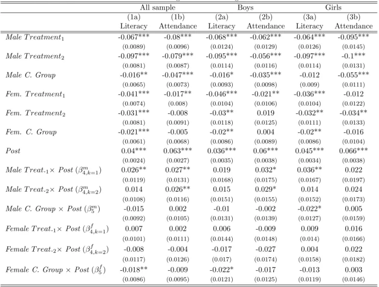
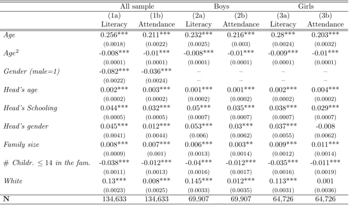
Table 4 has the results of specification (3) with schooling attendance or literacy as the dependent variables. Columns (1a) and (1b) show the results for regressions with the entire sample of children between 6 and 18 years old who live in rural areas. As expected, children living in treated families are in general less likely to be literate and attending school, since they are on average poorer families. Again, the coefficients of the control variables are all significant with the expected sign, reflecting the results found in the income regressions. Children living with an older, male, more educated and white head show better schooling outcomes. By the same token, the number of children in the family has a negative impact on education. The P ost coefficient captures the big positive trend in both attendance and literacy in the period for the whole sample.
The difference-in-difference coefficients show that the presence of an eligible male in the family had a positive and significant effect on the schooling achievements. Children living with a newly eligible male (Tm
k=1) are 2.6% and 2.7% more likely to be literate and attending school, respectively, while children with an old eligible male (Tm
k=2) are also significantly more likely to attend school (2.7%). On the other hand, despite causing a bigger increase in the family income, the presence of an eligible female does not seem to have improved the schooling outcome of the children. Neither the presence of a newly (Tkf=1) or an old (Tkf=2) eligible females has a positive effect on literacy or attendance. Actually, the presence of an old eligible female seems to decrease the likelihood of being literate.
Breaking the sample between boys and girls, we find positive effects in attendance for bothTm
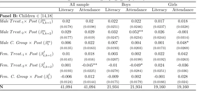
Table 5 shows the results after splitting the sample into two different subgroups: younger children between 6 and 14 and older children between 14 and 18. It is clear that the first group benefited much more from the reform than the second, especially the Tm
k=1 children; however, Tm
k=2 older boys also suffered a significantly positive effect on attendance. Again, children with an eligible female seem to have not benefited from the reform, at least compared to those in the reference group.
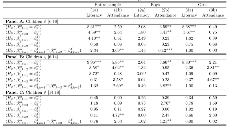
The last rows of each panel show the joint F-test if the presence of an eligible male is significant different from the presence of an eligible female in the family. Panel (A) shows the results for the regressions with the entire sample; Panel (B) and (C) show the results for children between 6 and 14; and 14 and 18, respectively. We can see that in all samples the presence of an eligible male had a significantly bigger effect than the presence of a female, especially for boys’ attendance. These results indicate that the families are not pooling their income and deciding the provision of those public goods based on the total family income; if that were the case there would be no reason why the presence of an eligible male would have a different impact on schooling than the presence of an eligible female. Thus, the findings contradict the core of the unitary model, i.e., the “neutrality” property.
Table 2) shows the proportion of people self-reported as ill and the proportion who have looked for any health care service in two points of time, before and after the reform. Like the schooling indicators, it displays a clear improvement on the heath indicators. In 1991, the Brazilian government created the SUS (The Universal Health System), which proposed to offer free health care for virtually every citizen in the entire country. Before that, only workers (and their dependents) who contributed to the social security system had access to the public health system. Since the implementation of the SUS coincides with the reform in the social security, our results could be very sensitive to it. The consistency of our estimation hinges on the assumption that the impact of the SUS creation was uniform across treated
and control groups. Once again, this example also testifies to the importance of having a control group (like the almost-eligible families) as similar as possible to the treatment one.
search for health care services, there is a negative correlation with age for both children and middle-agers. Again, the impact of the reform can be measured by the difference-in-difference coefficients (β4j,k). Looking at the results, we can see that the only significant impact of the reform was in the likelihood of being sick only for middle-agers who live with an old eligible male. Compared to thereference group, all other groups seem to have suffered no effect from any of the othertreatment groups.
The last row of table (9) tests whether there were different effects from the presence of eligible males and females. Once more, middle-age people who live with an eligible male significantly15 benefited more than those living with an eligible female.
Robustness Checks
As mentioned in section 4, thedifference-in-differenceestimator is consistent only ifreference
group has the same trend process as the treatment group in the absence of the treatment. For that reason, we included in the regressions a difference-in-difference estimator for the
control group - families with analmost-eligible member - in order to capture a possible trend associated with the presence of an elderly person in the family.
Table 6 shows the F-tests comparing thedifference-in-difference coefficients of both treat-ment against the control groups. Panel A has the tests for the entire sample while panels (B) and (C) displays the tests for children between 6 and 14, and 14 and 18 years old, respec-tively. Looking across the three different panels, we observe that the results are, in general, similar to those found when comparing to thereference group. The presence of eligible males seems more valuable than eligible females; and children between 6 and 14 years old benefited more from the reform than the older ones. In the same way, the results shown on table 9 corroborate the findings about health: middle-agers living with a newly eligible male are significantly less likely to be ill after the reform.
One possible caveat of the intent-to-treat approach rises if the take-up ratios for males and females are very different from each other. In this case, all uneven impacts of males and females shown in the main results could be driven by differences in the take-up ratios. One way to test if that is the case is to see the effects of the true treatment and compare to the intent-to-treat ones. Defining a treated group as the families that have a member who is an eligiblepensioner (i.e. there is a person in the family who receives a pension and matches the age eligibility criteria), we run specification 2 regressions using both definitions
15
of treatment. For both health and schooling, there is no significant difference between those two strategies. The results are qualitatively very similar, showing again a much bigger effect from the male presence compared to the female. The results are available upon request.
Income × Bargaining Effects
Case and Deaton (1998) show that one way to test if the pension income has the same impact as any other income source is by doing the following decomposition of total family income effect on the outcome of interest:
ln[In+φIp] = ln[I + (φ−1)Ip]≈ln(I) + (φ−1)Ip/I (4)
where In is the family non-pension income; Ip is the pension income; and, I is the total
family income.
We then need to test if the coefficient of the pension income share over the total family income (Ip/I) is different from zero. If that is the case, φ 6= 1 and, thus, the pension
money has a different effect on the public good provision than the rest of the family income. Moreover, this specification is also a direct test of the “neutrality” property of the public good. Non-zero coefficients on the income shares confirm the influence of the bargaining power in the decision-making process over the public good allocation within the family.
only male pensioners compare to those that have only female pensioners. Nevertheless, narrowing down our sample only to families with both female and male pensioners (Panel (C)) does not change the main conclusion that male pension share is more important for schooling attendance, especially for boys.
In the case of illness, the same conclusions arise. As expected total family income has a negative effect on the likelihood of being ill, and the male pension income share has a significant and bigger impact on the reduction of illness for middle-agers (table 10). Reducing the sample only to treated families (Panel (B)) diminishes the precision of the estimators without changing their signs.16 The same occurs in the sample including only families with both male and female pensioners (Panel (C)).
6
Conclusion
The social security reform occurred in 1991 in Brazilian rural pension system has led to an increase in schooling indicators for young children living with an eligible male. Boys are more likely to attend school and girls to be literate. The reform has also negatively impacted the probability of being ill on middle-age people living with a male pensioner. These uneven results for the presences of male and female recipients are evidence that the unitary model of household resource allocation does not represent the Brazilian poor rural families’ decision-making process over their budget. The income is not pooled and provision of education and health is not made based upon the total family resources. Moreover, we find an indication that the impact of the pension income on the schooling and health was higher than the rest of the family resources. The increase in the bargaining power of the elderly, especially males, may explain these findings, suggesting that they have stronger preferences toward those outcomes. The results show the importance of targeting specific family members in cash transfer programs in order to maximize the effect on desirable outcomes. Although families with an elderly person have on average low schooling and health indicator levels, cash transfers to those members of the family have significantly larger effects than unconditional transfers. In addition, since more than 10% of all children in rural areas live with an eligible person, it is very plausible to attribute part of the success Brazil has achieved in the past 15 years in education and health, specially for poor families, to the social security reform of 1991.
16
The findings have also great consequences for the design of conditional cash transfer programs, such asBolsa Escola andBolsa Familia. Those programs directly create incentives for schooling by requiring attendance. They set the mother as the receiver of the transfer. To the best of my knowledge, there is no study providing evidence that this is the most efficient away (in the sense of maximizing the outcome of interest). Therefore, a more profound study with the targeted families is necessary to identify specific members who may boost the direct income effect on schooling outcomes, enhancing the effectiveness of the programs.
A straightforward extension for this paper is to measure the impact of the reform on many other social outcomes, like child labor, fertility, anthropometrics, and other finer health indicators.
References
Becker, G. S.(1964) Human capital. Columbia Press University.
Becker, G. S. (1974) “A Theory of Social Interactions.” Journal of Political Economy
82(6): pp. 1063–93. Available at http://ideas.repec.org/a/ucp/jpolec/v82y1974i6p1063-93.html.
Becker, G. S.(1981) A Treatise on the Family. Harvard University Press.
Beltrao, K. I., et al.(2003) “The 1988 Constitution and Acess to Social Security in Rural Brazil: Towards Universalization.”
Bergstgrom, T. (1983) “Independence of Allocative Efficiency from Distribution in the Theory of Public Goods.” Econometrica 51: pp. 1753–1766.
Bergstgrom, T. and Cornes, R. (1981) “Gorman and Musgrave are Dual: An
An-tipodean Thoerem on Public Goods.” Economic Letters pp. 371–378.
Carvalho, I. E. (2000) “Old-age benefits and the labor supply of rural elderly in Brazil.” Mimeo.
Case, A. and Deaton, A.(1998) “Large Cash Transfers to the Elderly in South Africa.”
The Economic Journal 108: pp. 1330–1361.
Chiappori, P.-A. (1992) “Collective Labor Supply and Welfare.”
Journal of Political Economy 100(3): pp. 437–67. Available at
http://ideas.repec.org/a/ucp/jpolec/v100y1992i3p437-67.html.
Delgado, G. C. (1997) “Previdencia Rural - Relatorio de Avaliacao Socio-economica.” Texto para Discussao - IPEA 477.
Delgado, G. C. E. (1999) “Experiencias Exitosas de Combate a Pobreza Rural: Licoes para Reorientacoes de Politicas.” Projeto FAO Pobreza - LOA 98290/RLC.
Duflo, E.(2003) “Grandmothers and Granddaughters: Old-Age Pensions and Intrahouse-hold Allocation in South Africa.”World Bank Economic Review 17(1): pp. 1–25. Available at http://ideas.repec.org/a/oup/wbecrv/v17y2003i1p1-25.html.
Emerson, P. M. and Souza, A. P. (2007) “Bargaining over Sons and Daughters: Child Labor, School Attendance and Intra-Household Gender Bias in Brazil.” World Bank Economic Review (0213). Available at http://ideas.repec.org/p/van/wpaper/0213.html (forthcoming).
Ermisch, J. (2003) An Economic Analysis of the Family. Princeton Univerity Press.
Figures and Tables
Figure 2: Total family income (by gender) -in 2002 R$
Figure 4: Fraction of family income provided by eligible/almost-eligible person
Table 1: Literacy and Attendance (in %)
Panel A:Literacy
Before reform After reform 1988 1989 1990 1992 1993 1995 Children w/ an eligible person 51.58 54.76 56.39 57.4 58.82 65.07 Children w/ acontrol group person 58.42 59.82 62.23 61.92 62.64 68.2
Other children 51.66 52.98 53.8 57.37 60.07 63.36
All Boys 48.04 50.68 50.82 53.51 55.97 59.59
All Girls 56.70 57.14 59.22 62.13 64.43 68.80
Panel B:Attendance
Before reform After reform 1988 1989 1990 1992 1993 1995 Children w/ an eligible person 58.16 58.42 59.41 64.51 66.07 71.51 Children w/ acontrol group person 58.72 58.19 60.06 60.85 63.04 70.64
Other children 64.92 65.1 64.51 68.02 72.63 76.14
All Boys 62.13 62.48 61.51 64.93 68.81 73.09
All Girls 64.86 64.94 65.48 68.88 72.97 77.08
% of children (≥5 and≤15).
Table 2: Health Care and Illness (in %)
Panel A:Health Care
Before reform After reform
1986 1998
Everyone w/ an eligible person 8.77 11.11
Everyone w/control group 7.46 9.47
Other people 7.76 9.1
Boys w/ an eligible person 6.73 8.3
Girls w/ an eligible person 10.82 14.15
Middle-agers w/ an eligible person 8.04 11.29
Panel B:Illness
Before reform After reform
1986 1998
Everyone w/ an eligible person 9.47 8.34
Everyone w/control group 7.19 6.94
Other people 6.43 5.07
Boys w/ an eligible person 8.61 7.72
Girls w/ an eligible person 10.34 9.01
Panel A - % of people that looked for heath care in the past 2 weeks.
Table 3: Regression: total family income (in logs)
Variable Coefficient
MaleT reatment1 -0.133***
(0.0205)
MaleT reatment2 -0.11***
(0.0158)
Male C. Group -0.077*** (0.0181)
Fem. T reatment1 -0.074***
(0.0149)
Fem. T reatment2 -0.079***
(0.014)
Fem. C. Group -0.052*** (0.0164)
Post -0.125***
(0.0068)
MaleT reat.1×Post(β4m,k=1) 0.151***
(0.0262)
MaleT reat.2×Post(β4m,k=2) 0.302***
(0.0166)
Male C. Group×Post(βm
5 ) -0.033
(0.0253)
FemaleT reat.1×Post(β
f
4,k=1) 0.232***
(0.019)
FemaleT reat.2×Post(β
f
4,k=2) 0.443***
(0.016)
Female C. Group×Post(β5f) 0.041*
(0.023)
Head’s age 0.041*** (0.0011)
Head’s age squared -0.0003*** (0.00001)
Head’s schooling 0.138*** (0.0013)
Head’s gender 0.242*** (0.0105)
Family size 0.227*** (0.0026) #Childr. ≤14 in the fam. -0.251***
(0.0033)
Head is white 0.215*** (0.0058)
N 87,386
Robust standard errors in parenthesis.
Table 4: Regression: schooling
All sample Boys Girls
(1a) (1b) (2a) (2b) (3a) (3b)
Literacy Attendance Literacy Attendance Literacy Attendance
MaleT reatment1 -0.067*** -0.08*** -0.068*** -0.062*** -0.064*** -0.095***
(0.0089) (0.0096) (0.0124) (0.0129) (0.0126) (0.0145) MaleT reatment2 -0.097*** -0.079*** -0.095*** -0.056*** -0.097*** -0.1***
(0.0081) (0.0087) (0.0114) (0.0116) (0.0114) (0.0131) Male C. Group -0.016** -0.047*** -0.016* -0.035*** -0.012 -0.055***
(0.0065) (0.0073) (0.0093) (0.0098) (0.009) (0.0111) Fem. T reatment1 -0.041*** -0.017** -0.046*** -0.021** -0.036*** -0.012
(0.0074) (0.008) (0.0104) (0.0106) (0.0104) (0.0122) Fem. T reatment2 -0.031*** -0.008 -0.03** 0.019 -0.032** -0.034**
(0.0081) (0.0091) (0.0118) (0.0125) (0.0111) (0.0133) Fem. C. Group -0.021*** -0.005 -0.02** 0.004 -0.02** -0.016
(0.0061) (0.0068) (0.0086) (0.0089) (0.0086) (0.0104)
Post 0.04*** 0.063*** 0.036*** 0.06*** 0.045*** 0.066***
(0.0024) (0.0027) (0.0035) (0.0038) (0.0034) (0.0038) MaleT reat.1×Post(β4m,k=1) 0.026** 0.027** 0.019 0.032* 0.036** 0.022
(0.0119) (0.0131) (0.0168) (0.0175) (0.0167) (0.0197) MaleT reat.2×Post(β4m,k=2) 0.014 0.026** 0.015 0.029* 0.014 0.024
(0.0108) (0.0116) (0.0151) (0.0155) (0.0152) (0.0173) Male C. Group ×Post(βm
5 ) -0.015 0.002 -0.01 -0.002 -0.022* 0.005
(0.0092) (0.0105) (0.0131) (0.0139) (0.0127) (0.0159) FemaleT reat.1×Post(βf4,k=1) 0.007 0.002 0.006 -0.009 0.009 0.016
(0.0101) (0.0111) (0.0144) (0.0148) (0.014) (0.0166) FemaleT reat.2×Post(β
f
4,k=2) -0.008 -0.004 -0.017 -0.027 0.004 0.022
(0.0117) (0.0126) (0.017) (0.0174) (0.0158) (0.0182) Female C. Group ×Post(β5f) -0.018** -0.009 -0.022* -0.017 -0.013 0.003
(0.0086) (0.0095) (0.0121) (0.0125) (0.0119) (0.0146)
Table 4: Regression: schooling (cont.)
All sample Boys Girls
(1a) (1b) (2a) (2b) (3a) (3b)
Literacy Attendance Literacy Attendance Literacy Attendance
Age 0.256*** 0.211*** 0.232*** 0.216*** 0.28*** 0.203***
(0.0018) (0.0022) (0.0025) (0.003) (0.0024) (0.0032)
Age2
-0.008*** -0.01*** -0.008*** -0.01*** -0.009*** -0.01***
(0.0001) (0.0001) (0.0001) (0.0001) (0.0001) (0.0001) Gender (male=1) -0.082*** -0.036*** – – – –
(0.0022) (0.0024) – – – –
Head’s age 0.002*** 0.003*** 0.001*** 0.001*** 0.002*** 0.004***
(0.0002) (0.0002) (0.0002) (0.0002) (0.0002) (0.0002) Head’s Schooling 0.044*** 0.032*** 0.05*** 0.035*** 0.038*** 0.029***
(0.0005) (0.0005) (0.0007) (0.0007) (0.0007) (0.0007) Head’s gender 0.045*** 0.012*** 0.053*** 0.03*** 0.037*** -0.008
(0.0041) (0.0044) (0.006) (0.0062) (0.0055) (0.0062) Family size 0.008*** 0.007*** 0.006*** 0.003** 0.009*** 0.011***
(0.0009) (0.001) (0.0013) (0.0014) (0.0012) (0.0014)
#Childr. ≤14 in the fam. -0.038*** -0.012*** -0.04*** -0.012*** -0.035*** -0.011***
(0.0011) (0.0013) (0.0016) (0.0017) (0.0016) (0.0019) White 0.13*** 0.008*** 0.145*** 0.012*** 0.113*** 0.001
(0.0023) (0.0025) (0.0033) (0.0035) (0.0031) (0.0036)
N 134,633 134,633 69,907 69,907 64,726 64,726
Robust standard errors in parenthesis.
∗∗∗Significant at 1%;∗∗ Significant at 5%;∗Significant at 10%
Table 5: Regression: schooling - by age group
All sample Boys Girls
Literacy Attendance Literacy Attendance Literacy Attendance
Panel A: Children∈[6,14]
Male T reat.1×Post(βm4,k=1) 0.035** 0.039** 0.024 0.052** 0.049** 0.026
(0.0161) (0.0172) (0.0227) (0.0243) (0.0226) (0.0243) Male T reat.2×Post(βm4,k=2) 0.007 0.027* 0.008 0.021 0.007 0.034
(0.0136) (0.0143) (0.0192) (0.0203) (0.0191) (0.0202) Male C. Group ×Post(βm
5 ) -0.026** -0.011 -0.02 -0.004 -0.031* -0.018
(0.0125) (0.0133) (0.0179) (0.0185) (0.0173) (0.0191) Female T reat.1×Post(β
f
4,k=1) 0.013 -0.009 0.018 -0.012 0.009 -0.004
(0.0144) (0.0153) (0.0204) (0.0218) (0.02) (0.0213) Female T reat.2×Post(β
f
4,k=2) -0.01 0.015 -0.02 -0.016 -0.001 0.046**
(0.0145) (0.015) (0.0214) (0.0219) (0.0197) (0.0205) Female C. Group ×Post(β5f) -0.02* -0.021* -0.025 -0.029 -0.017 -0.012
(0.0119) (0.0124) (0.0169) (0.0173) (0.0165) (0.0179)
N 93,539 93,539 47,973 47,973 45,566 45,566
Table 5: Regression: schooling - by age group (cont.)
All sample Boys Girls
Literacy Attendance Literacy Attendance Literacy Attendance
Panel B:Children∈[14,18]
MaleT reat.1×Post(β4m,k=1) 0.02 0.02 0.022 0.022 0.017 0.018
(0.0178) (0.0198) (0.0251) (0.0246) (0.0237) (0.0328) MaleT reat.2×Post(β4m,k=2) 0.029 0.029 0.032 0.052** 0.026 -0.001
(0.0177) (0.019) (0.0247) (0.0234) (0.0244) (0.0314) Male C. Group×Post(βm
5 ) 0.006 0.022 0.007 0.004 0.001 0.048*
(0.0135) (0.0163) (0.0193) (0.0203) (0.0173) (0.0269) Fem. T reat.1×Post(β4f,k=1) 0.01 0.018 0.003 0.002 0.022 0.042
(0.0145) (0.016) (0.0207) (0.0199) (0.0192) (0.0263) Fem. T reat.2×Post(β
f
4,k=2) 0.001 -0.045** -0.01 -0.049* 0.024 -0.036
(0.0193) (0.0225) (0.0278) (0.0284) (0.0251) (0.036) Fem. C. Group×Post(β5f) -0.006 0.012 -0.009 0.002 -0.001 0.028
(0.0124) (0.0144) (0.0175) (0.0179) (0.0166) (0.024)
N 41,094 41,094 21,934 21,934 19,160 19,160
Robust standard errors in parenthesis.
∗∗∗Significant at 1%;∗∗ Significant at 5%;∗Significant at 10%
Table 6: F-Tests - schooling
Entire sample Boys Girls
(1a) (1b) (2a) (2b) (3a) (3b)
Literacy Attendance Literacy Attendance Literacy Attendance
Panel A: Children∈[6,18]
(H0:β4m,k=1=β
m
5 ) 8.31*** 2.59 2.08 3.59** 8.68*** 0.49
(H0:β4m,k=2=β
m
5 ) 4.59** 2.64 1.80 3.41** 3.67** 0.75
(H0:β
f
4,k=1=β
f
5) 4.10** 0.61 2.49 0.23 1.82 0.39
(H0:β
f
4,k=2=β
f
5) 0.50 0.08 0.05 0.23 0.75 0.68
(H0:β4m,k=1=β
f
4,k=1∩β
m
4,k=2=β
f
4,k=2) 2.34 3.69** 1.45 6.12*** 1.00 0.03
Panel B:Children∈[6,14]
(H0:β4m,k=1=β
m
5 ) 9.96*** 5.85** 2.64 3.86** 8.80*** 2.21
(H0:β4m,k=2=β
m
5 ) 3.58* 4.02** 1.32 0.95 2.36 3.81**
(H0:β
f
4,k=1=β
f
5) 3.72* 0.48 3.06* 0.47 1.09 0.09
(H0:β
f
4,k=2=β
f
5) 0.31 3.58* 0.04 0.23 0.37 4.67**
(H0:β4m,k=1=β
f
4,k=1∩β
m
4,k=2=β
f
4,k=2) 1.32 2.69* 0.49 3.82** 1.00 0.13
Panel C:Children∈[14,18]
(H0:β4m,k=1=β
m
5 ) 0.45 0.00 0.26 0.39 0.34 0.59
(H0:β4m,k=2=β
m
5 ) 1.18 0.09 0.73 2.76* 0.78 1.59
(H0:β
f
4,k=1=β
f
5) 0.95 0.11 0.27 0.00 1.02 0.19
(H0:β
f
4,k=2=β
f
5) 0.11 4.72** 0.00 2.47 0.66 2.30
(H0:β4m,k=1=β
f
4,k=1∩β
m
4,k=2=β
f
4,k=2) 0.76 2.53 1.02 4.21** 0.00 0.02
∗∗∗ Significant at 1%;∗∗ Significant at 5%;∗Significant at 10%
Table 7: Bargaining effect on attendance
All sample Boys Girls
Panel A:Entire Sample
Family Income (in logs) 0.022*** 0.025*** 0.019*** (0.0017) (0.0024) (0.0024)
Male pension / f. income 0.039*** 0.048** 0.03 (0.015) (0.0213) (0.0213)
Female pension / f. income 0.034** 0.031 0.034 (0.0169) (0.0249) (0.0231)
(H0: Male = Female Share) 0.005 0.017 0.004
(0.0345) (0.0542) (0.0478)
N 89,714 46,021 43,693
Panel B:Onlytreated families
Family Income (in logs) 0.04*** 0.037*** 0.042*** (0.0056) (0.0079) (0.008)
Male pension / f. income 0.128*** 0.134*** 0.122*** (0.0177) (0.0251) (0.0249)
Female pension / f. income 0.064*** 0.067** 0.058** (0.0196) (0.0286) (0.0268)
(H0: Male = Female Share) 0.064* 0.067** 0.064
(0.0375) (0.0312) (0.0457)
N 12,000 6,120 5,880
Panel C:Only families with both eligible male and female
Family Income (in logs) 0.042*** 0.045*** 0.039** (0.0124) (0.0174) (0.0177)
Male pension / f. income 0.107*** 0.163*** 0.05 (0.0365) (0.0534) (0.05)
Female pension / f. income 0.067 0.06 0.067 (0.0499) (0.0732) (0.0678)
(H0: Male = Female Share) 0.040 0.103** -0.017
(0.0564) (0.0497) (0.0785)
N 2,496 1,281 1,215
Robust standard errors in parenthesis.
Table 8: Regression: health
Entire sample Middle-agers Children Boys Girls
(1a) (1b) (2a) (2b) (3a) (3b) (4a) (4b) (5a) (5b)
Illness H.C. Illness H.C. Illness H.C. Illness H.C. Illness H.C.
MaleT reatment1 0.000 0.002 0.026 0.022 -0.007 -0.007 -0.008 -0.014 -0.007 0
(0.0053) (0.0053) (0.0216) (0.0229) (0.0084) (0.0077) (0.0118) (0.0098) (0.0121) (0.0119) MaleT reatment2 0.002 -0.005 0.05** 0.009 -0.007 -0.001 0 0 -0.015 -0.002
(0.0051) (0.0049) (0.0198) (0.0196) (0.0079) (0.0075) (0.0117) (0.0102) (0.0107) (0.0109) Male C. Group 0.002 -0.009** 0.013 0.024 0.004 -0.007 0 -0.002 0.008 -0.013
(0.0043) (0.0043) (0.0147) (0.017) (0.0072) (0.0062) (0.0099) (0.0093) (0.0104) (0.0082) Fem. T reatment1 -0.004 0.004 -0.002 -0.062** -0.015** 0.01 -0.011 0.01 -0.018* 0.01
(0.0044) (0.0044) (0.0266) (0.0198) (0.0075) (0.0083) (0.0112) (0.0113) (0.01) (0.012) Fem. T reatment2 -0.008 -0.007 -0.021 -0.032** -0.003 0.008 0.009 0.003 -0.017* 0.015
(0.0048) (0.0048) (0.0154) (0.0159) (0.0079) (0.0079) (0.0118) (0.0101) (0.0101) (0.0123) Fem. C. Group -0.001 0.007 0.004 -0.016 -0.007 0.007 -0.015 0.006 0 0.008
(0.0041) (0.0042) (0.0137) (0.0144) (0.0068) (0.0069) (0.0091) (0.0095) (0.0102) (0.0099)
Post -0.015*** -0.002 -0.003 0.002 -0.024*** 0.004 -0.025*** 0.005 -0.023*** 0.003
(0.0017) (0.002) (0.0064) (0.0072) (0.0023) (0.0028) (0.0032) (0.0039) (0.0034) (0.0041) MaleT reat.1×Post(β4m,k=1) -0.006 0.001 -0.042 0.026 0.004 0.013 0.006 0.012 0.003 0.014
(0.0071) (0.0079) (0.0272) (0.0335) (0.0116) (0.0129) (0.0161) (0.0172) (0.0165) (0.0191) MaleT reat.2×Post(β4m,k=2) -0.009 0.004 -0.056** -0.003 0.007 0.003 0.004 -0.003 0.011 0.01
(0.0063) (0.0063) (0.0221) (0.023) (0.0098) (0.0108) (0.014) (0.0144) (0.0138) (0.0164) Male C. Group×Post(βm
5 ) 0.001 0.012* 0.011 0.035 -0.013 0.016 -0.005 0.011 -0.02 0.021
(0.0059) (0.0063) (0.02) (0.0237) (0.009) (0.0103) (0.0123) (0.0147) (0.013) (0.0144) Fem. T reat.1×Post(β
f
4,k=1) 0.001 0.01 -0.008 -0.005 0.007 -0.001 0 0.005 0.014 -0.006
(0.0058) (0.0063) (0.0343) (0.0288) (0.0099) (0.0124) (0.0142) (0.0175) (0.0139) (0.0176) Fem. T reat.2×Post(β4f,k=2) 0.002 0.012* 0.006 0.015 -0.002 -0.014 -0.011 -0.01 0.01 -0.019
(0.0065) (0.0066) (0.0191) (0.021) (0.0103) (0.0112) (0.015) (0.0146) (0.0138) (0.0171) Fem. C. Group×Post(β5f) 0.009 -0.004 0.018 0.005 -0.001 -0.021** 0.006 -0.02 -0.008 -0.02
(0.0056) (0.0062) (0.0144) (0.016) (0.0086) (0.01) (0.0116) (0.0135) (0.0129) (0.0147)
Table 8: Regression: health (cont.)
Entire sample Middle-agers Children Boys Girls
(1a) (1b) (2a) (2b) (3a) (3b) (4a) (4b) (5a) (5b)
Illness H.C. Illness H.C. Illness H.C. Illness H.C. Illness H.C.
Age -0.001*** 0.000*** 0.014 -0.048** -0.007*** -0.021*** -0.007*** -0.021*** -0.006*** -0.020***
(0.0001) (0.0001) (0.0182) (0.021) (0.001) (0.0012) (0.0013) (0.0016) (0.0014) (0.0017)
Age2
0.000*** 0.000*** 0.000 0.001** 0.000*** 0.001*** 0.000*** 0.001*** 0.000* 0.001***
(0) (0.0000) (0.0002) (0.0002) (0.0001) (0.0001) (0.0001) (0.0001) (0.0001) (0.0001) Head’s age 0.000 -0.001*** 0.000 0.000 0.000* 0.000** 0.000 0.000 0.000* 0.000
(0.0001) (0.0001) (0.0005) (0.0005) (0.0001) (0.0002) (0.0002) (0.0002) (0.0002) (0.0002) Head’s Schooling -0.002*** 0.004*** -0.004*** 0.004*** -0.001*** 0.005*** -0.002** 0.004*** -0.001** 0.006***
(0.0003) (0.0003) (0.0009) (0.0011) (0.0004) (0.0005) (0.0005) (0.0007) (0.0006) (0.0008) Head’s gender -0.011*** 0.004 -0.027** -0.010 -0.008** 0.008* -0.012** 0.011* -0.005 0.004
(0.0027) (0.0029) (0.0097) (0.0105) (0.0039) (0.0043) (0.0055) (0.0058) (0.0055) (0.0063) Family size -0.005*** -0.005*** -0.003** 0.002 -0.003** -0.003*** -0.002* -0.003** -0.003** -0.003**
(0.0005) (0.0006) (0.0017) (0.002) (0.0008) (0.0009) (0.0011) (0.0012) (0.0012) (0.0013)
# Childr.≤14 0.006*** -0.001 0.005** -0.005** 0.003** -0.003** 0.002 -0.003* 0.004** -0.004**
(0.0007) (0.0007) (0.0024) (0.0026) (0.001) (0.0011) (0.0014) (0.0015) (0.0015) (0.0015) White 0.004* 0.009*** -0.004 0.010 0.008** 0.006 0.01** 0.01* 0.006 0.002
(0.002) (0.0025) (0.0066) (0.008) (0.0028) (0.0038) (0.0039) (0.0053) (0.004) (0.0054)
N 130,975 130,975 14,167 14,167 51,101 51,101 26,040 26,040 25,061 25,061
Robust standard errors in parenthesis.
∗∗∗Significant at 1%;∗∗Significant at 5%;∗Significant at 10%
Table 9: F-Tests - health
Entire sample Middle-agers Children Boys Girls
(1a) (1b) (2a) (2b) (3a) (3b) (4a) (4b) (5a) (5b)
Illness H.C. Illness H.C. Illness H.C. Illness H.C. Illness H.C.
(H0:β4m,k=1=β
m
5 ) 0.58 1.18 2.82* 0.06 1.54 0.05 0.35 0 1.34 0.11
(H0:β4m,k=2=β
m
5 ) 1.53 0.74 5.66** 1.47 2.44 0.84 0.21 0.5 2.79* 0.27
(H0:β
f
4,k=1=β
f
5) 1.22 2.87* 0.49 0.08 0.58 1.79 0.14 1.49 1.58 0.43
(H0:β
f
4,k=2=β
f
5) 0.59 3.07* 0.28 0.14 0 0.18 0.93 0.26 0.94 0
(H0:β4m,k=1=β
f
4,k=1∩β
m
4,k=2=β
f
4,k=2) 1.21 0.83 2.76* 0.05 0.06 1.29 0.36 0.16 0.09 1.44
∗∗∗Significant at 1%;∗∗Significant at 5%;∗Significant at 10%
Table 10: Bargaining effect on illness
All sample Middle-agers Children
Panel A:Entire Sample
Family Income (in logs) -0.014*** -0.021*** -0.009*** (0.0003) (0.0009) (0.0003)
Male pension / f. income -0.002 -0.033** 0.006 (0.0049) (0.0163) (0.0079)
Female pension / f. income 0.013** -0.012 -0.001 (0.0054) (0.0203) (0.0076)
(H0: Male = Female Share) -0.015* -0.021** 0.007
(0.0094) (0.0112) (0.0023)
N 126,208 13,704 48,483
Panel B:Onlytreated families
Family Income (in logs) -0.022*** -0.02*** -0.008*** (0.0007) (0.0025) (0.0011)
Male pension / f. income -0.009 -0.024 0.008 (0.0055) (0.0189) (0.0088)
Female pension / f. income 0.005 -0.005 0.006 (0.0062) (0.0238) (0.0089)
(H0: Male = Female Share) -0.014 -0.019* 0.002
(0.0105) (0.0119 (0.0231)
N 28,714 2,092 5,302
Panel C:Only families with both eligible male and female
Family Income (in logs) -0.024*** -0.025*** -0.009*** (0.0012) (0.0083) (0.0025)
Male pension / f. income -0.019** -0.063 0.019 (0.0084) (0.0563) (0.0197)
Female pension / f. income 0.039*** 0.002 0.005 (0.0123) (0.0837) (0.0238)
(H0: Male = Female Share) -0.058** -0.065* 0.014
(0.0249) (0.0380) (0.0523)
N 10,426 271 1,045
Robust standard errors in parenthesis.