Flypaper effect revisited: Evidence for tax collection efficiency in Brazilian
municipalities
Paulo Arvate
1, Enlinson Mattos
2and Fabiana Rocha
3Abstract
This paper has two purposes. First, to construct efficiency scores in tax collection for
Brazilian municipalities in 2004, taking into consideration two outputs: amount of per capita
local tax collected -tax revenue- and the size of local informal economy- tax base. This
methodology eliminates the price- effect of tax collection. Second, using the rules established
on the Brazilian Constitution in 1988 to transfer unconditional funds among municipalities
as instrument, to estimate the relationship between intergovernmental transfers and
efficiency in tax collection. We conclude that transfers affect negatively the efficiency in tax
collection, leading to a reinterpretation of the flypaper effect.
Keywords
: Flypaper effect, Efficiency, Tax collection, pressure groups
1. Introduction
The fiscal capacity of an economy can be defined as the potential ability of its governments to
raise revenues from its own sources to finance public goods and services. In other terms, fiscal
capacity corresponds to the potential ability of an economy to collect revenues. It is influenced by the
economic structure of the country, state or municipality, by the availability of taxable resources (tax
bases) and by the groups that demand public services within the unit.
There are a variety of methods to measure an economy’s fiscal capacity. The most obvious
one is to use revenue collections as a measure of fiscal capacity. Current revenue collections is
however a poor proxy for fiscal capacity. This measure does not recognize that the amount of revenue
collections is affected both by an economy’s fiscal capacity and its fiscal effort. Regions with a
smaller tax base will have a more limited potential ability to raise revenues but also will regions with
a larger tax base but low tax enforcement effort. Besides, the use of revenue collections as a measure
of fiscal capacity can imply a perverse incentive to economies to lower their fiscal effort. If the
central government decides that revenue collections should be the measure of fiscal capacity, and
therefore should be used in the allocation of equalization grants, regions would have an incentive to
collect less revenue from their own sources. The voters would be pleased with lower levels of
taxations, and the revenue shortfall would be offset by an increased level of transfers from the central
government.4 In addition, the political groups acting in the domestic scenario tend to affect the level
of public services provided and the tax effort of the municipalities, differently from the median voter.
A different approach would be to integrate revenue collections and availability of tax bases as
measures of the fiscal capacity in each municipality given the per-capita resources spent on that end.
The great advantage of the use of such indicators is that they take into account explicitly the monetary
effort for tax collection of each unit as inputs and two components of the fiscal capacity as outputs.
On the other hand, fiscal effort can be identified as the degree to which a government uses the
revenue bases available to it. It is affected by incumbents´ relation with their voters (median voter,
pressure groups, etc) which determine the level of the tax rates applied, the level of exemptions
granted, and the tax enforcement effort implemented by the tax administration authorities. The level
of fiscal effort is typically measured as the ratio of the actual amount of revenues collected to some
measure of fiscal capacity. From these two related concepts; one can calculate the fiscal potential of
an economy, which can be characterized as the maximum attainable revenues that would result if that
unit uses efficiently all its resources and ability to collect them. Fiscal potential can then be computed
as the tax collection resulting from the estimation of a fiscal possibility frontier. The fiscal frontier is
the collection (or a function) of those different tax potentials. The efficiency in tax collection is, then,
the distance to that fiscal frontier.
This issue is relevant in local economies in a context of fiscal federalism. These local
governments receive transfers from higher levels of the government which enables them to provide
efficiency in tax collection. That stresses the political importance of the pressure groups to obtain
such benefits from the local government.
The purpose of the paper is to investigate the effect of intergovernmental transfers on the
fiscal potential of 3,359 Brazilian municipalities in 2004. In particular we construct efficiency scores
in tax collection for each unit, taking into consideration two outputs: amount of per capita local tax
collected – revenue collection - and the proportion of workers on the local informal economy -
availability of tax bases. Next, to eliminate the endogeneity of these transfers, we build an instrument
for intergovernmental transfers using the rules established on the Brazilian Constitution in 1988 to
transfer unconditional funds among municipalities. The results suggest that federal transfers to
municipalities negatively affect the efficiency scores. This leads to a reinterpretation of the traditional
flypaper effect that suggests that transfers increase public spending (taxation) more than do increases
in private income. Here higher transfers from the federal government might induce less efficiency in
local tax collection5.
Although the empirical literature widely regards the flypaper effect as a refutation of the
government’s rationality, since it is argued that government’s allocation is different from that of
private agents in the presence of transfers, Becker (1996) has recently disputed its existence.6 She
argues that the ´´fiscal illusion`` of the flypaper effect is nothing but an econometric artifact, usually
associated with misspecification biases.7 This paper also addresses this issue and presents alternative
specifications of the main model.
The paper is organized in four sessions. The second session lays out briefly the existent
literature on the flypaper effect, and sets a simple model that restates its characteristics in terms of
efficiency of taxation, and not in terms of expenditure (taxation) levels. The third session introduces
the estimation procedures to be followed, provides the rationale for the construction of the
instrumental variable and presents the empirical estimates. The fourth session concludes.
2. The flypaper effect revisited
2.1. A simple model
This paper recognizes that intergovernmental transfers are determined through a political process
and that grant receipts is an outcome of the underlying preferences of the elected representatives. The
bargaining process can be formally reduced to two stages. First, there exists a ´´federal budgetary
stage`` which determines how to distribute an exogenous budget across municipalities. The second
stage considers the intergovernmental grant as given, and it consists in allocating these federal grants
and private income between public and private consumption. Since the first stage is the political
process which is being instrumented in our set up and described below, we only argue here that the
correlation between preferences for the public good and grant receipts can be positive, which
invalidates the direct use of these transfers in the regression analyses. Those transfers might be
correlated with unobservable political variables.8
Hamilton (1986) presents a simple model of optimal tax theory that focus on the deadweight loss
from taxation as the possible cause of the flypaper effect. The author postulates that grants allow
lower local taxes. In this paper, we extend Hamilton´s model by accommodating a tax collection
function in the local tax revenues. This seems to be a reasonable strategy since the main assumption
here is that only local taxation is distortionary, and that is this effect that local pressure groups
attempt to circumvent.
Formally, consider an economy with a composite good (Z), a locally provided public service (G),
and a representative agent.9 The government’s budget constraint contains two sources of revenues, T
which is the revenue from local taxes and t, an intergovernmental grant. The budget constraint is,
therefore,T +t≥G.
Assuming as in Hamilton (1986), that local taxes are distortionary, the individual’s budget
constraint can be written as y≤x+g(T), where y is real income and g(T) represent the shadow cost
of local taxes in terms of private consumption with the following properties: i) g(0)=0, ii)
1 ) ´(T >
g , and iii) g´´(T)>0if T > 010.
Now suppose a smooth and strongly quasi-concave household utility function which is increasing
in both of its arguments. It can be rewritten, after substituting both constraints, as
) ), (
(y g T T t U
U = − + (1)
This allows characterizing the solution of the local government as
0
)
´(
21
g
T
+
U
=
U
(2)A formal statement of the flypaper effect is that the marginal public expenditure due to a grant
(dG/dt =1+dT/dt) is greater than the marginal public expenditure arising from an equivalent
increase in total community income (dG/dy=dT/dy). This is mostly an empirical observation
that unrestricted grants from higher to lower levels of government stick where they land11.
We assume that the amount of taxes collected is a function of the inputs used to that end.
Specifically, that depends on how much capital and labor is employed to collect revenues to the
government12
)
,
(
i i ii
f
K
L
T
=
φ
(3)where i =1,…,n corresponds to the number of municipalities in Brazil and
φ
iis a parameter thatcaptures how efficient these inputs are combined to collect revenues.
Consider the total differentiation (omitting the subscripts on K and L),
i L
k i
i
f
K
L
f
dK
f
dL
dT
d
φ
(
,
)
+
φ
[
+
]
=
(4)Equation (4) reveals that in order to compensate an increase in local taxes, the municipalities can i)
size to collect tax revenue (capital and labor) depends on the municipalities’ choice regarding the
allocation of resources to tax collection. For instance, it could be the case that local governments
suffer pressures from specific groups whose aim is to obtain exemptions (elderly, poor, etc). To attain
that claim, local governments can reduce the number of workers allocated to auditing, or to decrease
investments that can help in the tax collection such as electronic tax payment system and record
which connects its data basis with their counterparts in different spheres of the government.
To consider the partial effect of a change in the amount of transfer (t), and the amount of own
income (y), on the efficiency scores, totally differentiate equation (2) and use equation (4) to obtain
)
,
(
]
´
2
´´
´
[
´
22 12 1 2 11 22 12L
K
f
U
g
U
g
U
g
U
U
g
U
dt
d
i+
−
−
−
=
φ
(5))
,
(
]
´
2
´´
´
[
´
22 12 1 2 11 12 11L
K
f
U
g
U
g
U
g
U
U
g
U
dy
d
i+
−
−
−
=
φ
(6)The ´´flypaper effect`` on the efficiency score is the result of
)
,
(
]
´
2
´´
´
[
)
´
(
)
´
(
22 12 1 2 11 12 11 22 12L
K
f
U
g
U
g
U
g
U
U
g
U
U
g
U
dy
d
dt
d
i i+
−
−
−
−
−
=
−
φ
φ
(7)which is the difference between the effect of transfer and income effect on the efficiency side of tax
collection. The denominator of equation (7) is negative since it is the second derivative of the
government budget’s constraint. Therefore, the final effect can be positive or negative depending on
the relative sign of
(
U
12g
´
−
U
22)
and(
U
11g
´
−
U
12). In order to have a negative flypaper effect on efficiency scores, that is, equation (7) lower than zero, a sufficient conditionis
(
U
12g
´
−
U
22)
−
(
U
11g
´
−
U
12)
>
0
. Since the second term of the numerator(
U
11g
´
−
U
12) is negative, once it is assumed that the public good is normal (dG/dy>0) (leads to equation (6) to be positive), thisis equivalent to have either a positive or low negative value for the term
(
U
12g
´
−
U
22)
. In particular, a sufficient condition can be written as(
U
12g
´
−
U
22)
<
(
U
11g
´
−
U
12)
13.
This means a lower effect, in absolute terms, on efficiency scores of grants than that one
caused by income variation. This is what we label new flypaper effect , that is, the difference in the
effect of transfers on tax collection efficiency compared to the standard effect of transfers on
spending.
3. Empirical procedure
The goal of the first stage is to construct a tax frontier. It is similar to a production frontier in
the firm’s problem of producing output. The government problem is to generate taxes, and it is
concerned with its tax potential. In other terms, the idea is to measure the “wastefulness” of taxation.
As observed by Alfirman (2003) the difference between the fiscal frontier and current taxation
can not be considered strictly as a measure of inefficiency, representing in fact the level of unused tax
potential. Given that the existence of unused tax potential may also be caused by the preference of
municipalities’s residents (they voluntarily prefer a low provision of public goods and services),
inefficiency is only part of the story. We totally understand this point but we will use the term
inefficiency from now on.
In a frontier framework it is possible to rank the efficiency of tax collection by comparing
each municipality fiscal performance with a tax frontier (fiscal potential). Along the tax frontier it is
observed the highest possible level of output (revenue collection) for a given level of input.
Conversely, it is possible to determine the lowest level of input necessary to attain a given level of
output. This way it is possible to identify inefficient procedures in terms of input efficiency and in
terms of output efficiency.
The second stage goal is to identify the variables correlated with inefficiency scores across
municipalities. Given that the dependent variable, the efficiency scores, is continuous and distributed
over a limited interval (between zero and one) we present in addition to OLS estimates, a censored
Tobit regression model to verify its relationship with the independent variables.
We estimate the following tax collection efficiency function :
i i
i o
i
Transf
Income
Controls
EffScore
=
β
+
β
1+
β
2+
γ
+
ε
(8)where EffScorei corresponds to the computed efficiency score for municipality i., Transf is our
variable of interest and measures the amount of transfers received by municipality i., Incomei is the
per-capita income of that municipality, and Controls represent a vector of other variables that are
believed to explain efficiency (see below.).
The local government, however, may have incentives to collect less revenue from their own
sources in order to receive higher transfers. Or at least they can be less efficient in tax collection if
that action can imply higher grants received. This is a typical endogeneity problem in econometrics
and we attempt to solve it by building an instrumental variable. This variable must be correlated with
tax collection efficiency only through the instrumented variable, and not be correlated with the
residuals. This identification strategy is also attractive because of the possible selection on
“unobservables”, i.e., a municipality may be receiving a specific amount of transfers due to the
political power and groups of interest which are not observed by the researcher. The construction of
the instrument aims to eliminate these biases.
The Brazilian municipalities can decide upon fines, exemptions and tax rates on two specific
taxes: the service tax (ISS) and the residential property tax (IPTU). Another source of revenues is the
intergovernmental transfers that could come from the state and federal spheres.
Brazilian municipalities depend heavily on transfers as a source of revenues. According to the
Government Finance Statistics Yearbook, IMF, 2003, tax revenues represent only 24% of total
revenue in average for Brazilian municipalities. This large volume of transfers received by Brazilian
municipal governments led Shah (1994, p. 42) to argue that “municipal governments in Brazil (...)
should be the envy of all [local] governments in developing, as well as industrial countries”.
Given that the “rules” used to transfer resources from the states and central government to the
municipalities change constantly, these different rules turn the use of unconditional transfers as
instrument endogenous.14
From an historical perspective it is possible to see that the transference of resources from one
sphere to another in Brazil and the rules establishing their amount, are the result of either political
dissatisfaction with the current rule of distribution or take into account the change in the variables
used in the redistribution criteria over time. For instance, the actual rule of resources distribution
considers the level of population (the only criterion for municipalities other than states’ capitals) and
per-capita income (both are used in the case of capitals’).15 These two variables adjust annually for
Brazilian municipalities and consequently the coefficients of redistribution among municipalities
might adjust as well.
The problem is that these coefficients can be correlated with unobservable variables and
consequently with the decision of tax collection. In particular, if the variation of these two criteria
implies a decrease in the transfers’ participation of a particular municipality, they can claim an
attenuation of this loss. Depending on their political status (whether they are supported– amparado –
capitals or reserva) they can get a different formula for adjustment. Also, that formula has been
corrected three times since its first implementation16. Therefore, a municipality whose population
decreases (increases) does not have its participation in transfers´ funds automatically decreased
(increased) proportionally. There exists an ongoing process of verification of municipality’s political
status and which attenuation coefficients are applied. After that the municipalities can still complain
and negotiate over their classification and redistributive grants until 30 days after the final publication
of those data. Last, even municipalities with similar population and income per-capita might have
different coefficients because they belong to a different state. The states´ coefficients were fixed and
never changed by the Resolution 242/90, in 1990.17
As a consequence the final amount of transfers to each municipality may result from
unobservable characteristics of each municipality, including political groups of pressure or lobbying,
or still tax revenues and tax base that can be used as argument to receive more (or less) transfers.
Therefore it would be necessary to search for an instrumental variable that is associated with tax
capture unobservable effects. In addition, we have to make use of the control variables that capture
heterogeneous components of each municipality (economics, social and political).18
We use the result established in the 1998 Constitution as the benchmark to build up our
instrument. Although it was the last Constitutional reform in Brazil the coefficients of resources
redistribution among municipalities were established only in the complementary law 62 in 1989. In
particular, given any amount of revenues collected by the central government, this law presents the
coefficients of how they should be divided for each municipality in that year.19 The rule of
distribution of federal resources (unconditional grants) establishes coefficients that depend on the
level of population living in each municipality according to the population data published by the
Instituto Brasileiro de Geografia e Estatistica -IBGE (the Bureau responsible to estimate annually the
size of population on each municipality). However, since these coefficients associated to each of
municipality may change overtime, we use the one established for the first time, by the Law 62 in
1989. This law establishes eighteen individual coefficients – from 0,6 to 4 - depending on the size of
population, i.e. from less than 10.188 habitants to more than 156.216 habitants for the municipalities
in the countryside. Concerning the States´ capitals, ten percent of the total collected fund is
distributed proportionally to each one depending on its population (coefficients vary from 2 to 5) and
the inverse of per-capita income of its State (coefficients go from 0,4 to 2,5).
That generates a different distribution than the one characterized by the rule in 2004 and
eliminates the contemporaneous bias. This seems to be a valid instrument for two reasons: 1) This law
was established as part of a Constitutional reform, usually assumed to be exogenous in the literature20
and 2) This law is fifteen years old (comparing to 2004, our database) and has been changed often.
Therefore, it is reasonable to assume that any stock effect has been reduced.21
The instrument is build as follows. First, we collect data on federal government revenues that
come mostly from two taxes in 2004: income tax and a tax on industrialized products (IPI), which is a
consumer tax. Next, we multiply this amount by 22.5% to find the amount to be distributed to the
municipalities in 2004. According to 1988 Constitution, municipalities have to receive 22.5% of what
the central government collects from these taxes. Last, we multiply the resulting amount by the
individual coefficients mentioned above to obtain the specific amount of transfers to each
municipality. This amount corresponds to the instrument for transfer and we called it Transftab.
3.2 Data and Efficiency Scores
The variable of interest is the transfer from federal and state governments to the municipalities.
According to our theoretical model it could be the case that the higher these transfer, the higher the
level of inefficiency. A negative sign would imply that municipalities are extremely
revenue-dependent on such central and state government assistance, exploiting their tax potential only
partially. If this is the case, the central government should design a new transfer policy that would
influence municipalities to increase efficiency and use all their tax potential, reducing at a minimum
The control variables aim to capture specific characteristics of the municipalities such as
technology, municipalities characteristics, fiscal variables. We also include the ideology of mayors
and municipalities groups of interest22. The sources of the data are provided on the appendix.23
The literature mentions the effect of the ideology of the governments on taxation. Messere (1993)
argues that center-right governments generally tend to choose a lower total tax burden, with more
consumer taxes than income taxes. On the other hand, left-wing governments tend to favor a higher
size of the government which implies a higher tax burden, with more income taxes than consumption
taxes. Pommerehne and Scheneider (1983) analyze Australia during the 70s and argue that right-wing
governments tend to have less direct taxes and a lower tax/GDP ratio, while left-wing governments
tend to have more indirect tax and a higher tax/GDP ratio. Therefore, if a higher level of tax revenue
can lead to higher tax collection efficiency, we could expect a positive sign for the coefficient of the
dummy associated to left-wing governments.
As Sousa et al. (2005) argue, technology helps to increase efficiency. Although they are looking
at the expenditure side, the same applies to the revenue side. We use two dummy variables as proxies
for the existence of technology: electronic tax service data set (ISSinform), and the services from
municipalities to contributors through internet, portal or web page. The electronic tax collection can
help the local government to interact with higher spheres of the government when auditing
individuals.
We use the per capita income to represent the stage of development, following Lotz and Mors
(1967). They argue that usually the higher the stage of development, the higher the rate of literacy,
the higher the degree of monetization, and the stricter the law enforcement. All these factors are
expected to increase tax capacity, and could lead to higher tax collection efficiency. Also, the stage of
development captures the tax base, so more developed municipalities may have a bigger tax base
which impacts positively on tax potential. Finally, more developed municipalities probably need a
higher tax capacity in order to meet the higher amount of public expenditures that they probably have
to provide. Therefore we expect a positive sign for this variable.24 We also use the percentage of
people which have electric energy at home (Eletricity) , the percentage of the residents in the
municipality that own a computer (Computer), the size of the population (Population), and the density
of population (Density) as proxies for the stage of development.
Concerning the role of interest groups, Dougan and Kenyon (1988), argue that government
budgeting can divert the allocation of funds away from the one preferred by the median voter due to
lobbying made by interest groups.25 They show that when a subset of the population is lobbying for
an increase in local expenditures on an item, and if the municipality receives a categorical grant of
that item, then that grant increases the income of those individuals who contribute to the local
lobbying effort.26 This, in turn, tends to reduce the lobbying effort of that group, allowing for a
possible reduction in local taxes27. On the other hand, Rodríguez (2004) argues that “the bargain
income do not pay taxes”. In order to identify pressure groups with this characteristics we use the
percentage of people older than 65 living alone (Elderly); the percentage of people employed
(Employed), defined as the economically active population divided by the working age population;
the percentage of urban population over resident population (Urbanization). We expect that the
higher the percentage of people over 65 , the smaller the level of tax revenue, and the higher the
inefficiency, since they are usually exempted of municipality tax in Brazil. The higher the percentage
of people employed and the higher the degree of urbanization, the easier is to collect taxes. Therefore,
we would expect to observe a positive relationship between these variables and tax potential.
However, they do not want to be fiscally penalized and pressure for exemptions, for a greater fiscal
effort on the agricultural sector, and a decrease in informality. Therefore, we also expect these
variables to have an inverse relationship with tax potential and efficiency.
Last, the variable transp captures the distance in monetary terms from the actual city to the
closest state´s capital. It represents how far the municipalities with respect to the state bureaucracy
are. This bureaucracy could have an additional political power that imposes to local government more
visibility and efficiency in local tax collection. Consequently, we expect that variable to have a
negative relation with respect to tax collection efficiency
The characteristics of municipalities are summarized on Table 1.
Table1: Descriptive Statistics
output scores output scores output scores em p Incom e expenditures (tax revenue) ( proportion of inform al w orkers) (both)
M in. 0.010 0.000 0.015 0.250 30.430 102.100
1st Q 0.299 0.037 0.312 0.508 107.510 436.600
M edian 0.468 0.066 0.488 0.562 186.530 582.700
M ean 0.483 0.126 0.504 0.561 192.240 677.100
3rd Q 0.649 0.135 0.680 0.606 250.050 806.200
M ax. 1.000 1.000 1.000 0.932 954.650 6327.100
urbanization density eletricity com pu Transftab ISSinform
M in. 0.000 0.082 17.430 0.002 0.000 0.000
1st Q 43.200 12.920 87.920 0.998 211.292 0.000
M edian 62.740 26.030 96.580 2.621 275.602 1.000
M ean 61.410 119.500 90.340 3.962 370.596 0.696
3rd Q 81.090 54.040 99.250 5.445 448.678 1.000
M ax. 100.000 12700.000 100.000 41.405 2650.591 1.000
transp right transferences elderly IPTUinform left
M in. 0.000 0.000 193.100 0.056 0.000 0.000
1st Q 221.300 0.000 533.700 10.336 1.000 0.000
M edian 376.000 0.000 689.000 12.986 1.000 0.000
M ean 428.700 0.401 819.700 13.054 0.885 0.353
3rd Q 542.400 1.000 967.900 15.671 1.000 1.000
M ax. 5949.000 1.000 7775.900 28.698 1.000 1.000
Tax revenue and proportion of inform al workers denote Tax revenue and tax base criteria.
Concerning the efficiency scores computation, inputs are defined as capital and labor.28 We
use the capital investments per-capita from 1980 and 2004 accumulated and depreciated by the rate of
3% as a proxy for capital (K).29,30
These variables allow us to calculate input and output relative efficiency scores whose range
score 1. For instance, the input efficiency score of a unit means how much less input could be used to
obtain the same level of output. Similarly, the output efficiency score calculates how much more
output could be produced given the level of inputs.
This paper utilizes the Free Disposable Hull (FDH) methodology to compute those scores and
it is described on the appendix.31 The major advantage of FDH analysis is that it imposes only weak
assumptions on the production technology but still allows for comparison of efficiency levels among
producers. It is necessary to assume that reduction of the inputs (outputs) with the same technology
maintaining the output (input) fixed across municipalities are made. The production set is not
necessarily convex. That guarantees the existence of a continuous FDH which is going to be used as a
dependent variable to identify the best practices in government tax collection, that is, to asses what
are the factors increase (relative) efficiency. We claim that using such structure, allows us to exclude
the tax-price effect on the tax collection determinants. Suppose that we want to estimate the
determinants of tax collection in two similar units of observation. In one of them twice as much is
spent on tax collection activities compared to the other. If the two units are similar in their
characteristics, we expect to have the double amount of revenue collected in that unit whose
expenditure in tax collection is higher. That unit can audit more; can spend more money in training
the auditors, etc. We must take into consideration the cost/effort to collect tax in the municipalities to
compute the determinants of tax collection. The cost to collect tax is the price paid to generate tax
revenue and availability of tax base. By using FDH methodology, we rank the municipalities’ tax
collection activity considering their input (price).
The results are summarized on Table 2 below32.
Table 2: Efficient Scores: All and by State.
Sample (observations)
Input scores -proportion of
informal workers -Tax Base
Output scores -proportion of
informal workers -Tax Base
Input scores -Tax revenue
Output scores -Tax revenue
Input scores -both
Output scores -both Total (3359) min 0,017 0,010 0,017 0,000 0,017 0,015
max 1,000 1,000 1,000 1,000 1,000 1,000
mean 0,282 0,483 0,294 0,126 0,322 0,504
std 0,185 0,236 0,189 0,168 0,215 0,243
Amapá(37) min 0,063 0,091 0,063 0,009 0,063 0,108
max 0,930 0,882 0,930 0,738 0,930 0,882
mean 0,327 0,466 0,300 0,095 0,333 0,472
std 0,202 0,192 0,193 0,137 0,206 0,191
Acre (15) min 0,065 0,034 0,065 0,001 0,065 0,038
max 1,000 1,000 1,000 1,000 1,000 1,000
mean 0,198 0,350 0,198 0,081 0,198 0,352
std 0,231 0,232 0,231 0,255 0,231 0,231
Amazonas (42) min 0,048 0,045 0,048 0,008 0,048 0,057
max 1,000 1,000 1,000 1,000 1,000 1,000
mean 0,183 0,251 0,199 0,077 0,199 0,257
std 0,166 0,182 0,184 0,195 0,184 0,184
max 1,000 1,000 1,000 1,000 1,000 1,000
mean 0,395 0,470 0,402 0,282 0,402 0,521
std 0,268 0,246 0,261 0,339 0,261 0,254
Pará (22) min 0,027 0,034 0,040 0,005 0,040 0,039
max 1,000 1,000 1,000 1,000 1,000 1,000
mean 0,228 0,335 0,252 0,117 0,256 0,351
std 0,206 0,241 0,202 0,205 0,201 0,238
Amapá (3) min 0,265 0,182 0,265 0,088 0,265 0,219
max 0,657 0,714 0,657 0,115 0,657 0,733
mean 0,441 0,488 0,424 0,100 0,441 0,506
std 0,199 0,275 0,206 0,014 0,199 0,263
Tocantins (50) min 0,017 0,065 0,017 0,001 0,017 0,081
max 0,561 0,831 0,594 0,524 0,594 0,842
mean 0,174 0,263 0,202 0,078 0,206 0,286
std 0,118 0,146 0,135 0,089 0,142 0,148
Maranhão (47) min 0,047 0,015 0,047 0,000 0,047 0,031
max 1,000 1,000 1,000 1,000 1,000 1,000
mean 0,348 0,251 0,367 0,106 0,367 0,263
std 0,225 0,210 0,251 0,214 0,251 0,217
Piauí (85) min 0,028 0,011 0,028 0,007 0,028 0,032
max 0,614 0,739 0,834 0,538 0,834 0,850
mean 0,222 0,201 0,236 0,043 0,236 0,211
std 0,152 0,135 0,171 0,062 0,171 0,138
Ceará (115) Min 0,036 0,013 0,036 0,006 0,036 0,029
Max 0,572 0,794 0,799 0,762 0,960 0,831
Mean 0,228 0,254 0,239 0,059 0,241 0,264
Std 0,126 0,137 0,139 0,082 0,145 0,135
Rio Grande do Norte
(93) Min 0,032 0,071 0,032 0,009 0,032 0,080
Max 0,768 0,984 1,000 1,000 1,000 1,000
Mean 0,226 0,384 0,240 0,068 0,243 0,396
Std 0,121 0,162 0,140 0,107 0,138 0,166
Paraíba (105) Min 0,024 0,012 0,030 0,006 0,030 0,029
Max 0,555 0,839 0,722 0,511 0,722 0,839
Mean 0,246 0,315 0,256 0,052 0,258 0,324
Std 0,098 0,170 0,103 0,054 0,103 0,167
Pernambuco (122) Min 0,034 0,015 0,034 0,005 0,034 0,043
Max 0,988 0,966 1,000 1,000 1,000 1,000
Mean 0,327 0,382 0,325 0,074 0,335 0,390
Std 0,152 0,216 0,146 0,113 0,157 0,216
Alagoas (73) Min 0,066 0,023 0,066 0,001 0,066 0,029
Max 0,676 0,824 0,676 0,594 0,676 0,848
Mean 0,286 0,364 0,291 0,048 0,293 0,369
Std 0,118 0,155 0,117 0,075 0,118 0,155
Sergipe (45) Min 0,024 0,104 0,045 0,008 0,045 0,114
Max 1,000 1,000 0,621 0,448 1,000 1,000
Mean 0,251 0,403 0,249 0,070 0,267 0,419
Std 0,203 0,198 0,150 0,085 0,205 0,205
Bahia (154) Min 0,024 0,057 0,055 0,005 0,055 0,068
Max 1,000 1,000 1,000 1,000 1,000 1,000
Mean 0,290 0,366 0,316 0,095 0,317 0,383
Std 0,146 0,176 0,160 0,140 0,160 0,187
Minas Gerais (503) Min 0,022 0,010 0,031 0,000 0,031 0,015
Max 1,000 1,000 1,000 1,000 1,000 1,000
Std 0,166 0,229 0,154 0,120 0,184 0,235
Espírito Santo (58) Min 0,023 0,182 0,023 0,015 0,023 0,187
Max 1,000 1,000 1,000 1,000 1,000 1,000
Mean 0,298 0,537 0,309 0,131 0,338 0,554
Std 0,162 0,186 0,160 0,176 0,192 0,195
Ro de Janeiro (62) Min 0,030 0,297 0,051 0,027 0,051 0,297
Max 1,000 1,000 1,000 1,000 1,000 1,000
Mean 0,328 0,652 0,411 0,305 0,436 0,710
Std 0,257 0,172 0,264 0,287 0,281 0,178
São Paulo (460) Min 0,020 0,170 0,024 0,008 0,024 0,187
Max 1,000 1,000 1,000 1,000 1,000 1,000
Mean 0,332 0,640 0,416 0,261 0,438 0,677
Std 0,202 0,180 0,246 0,251 0,258 0,194
Paraná (308) Min 0,019 0,102 0,024 0,014 0,024 0,122
Max 0,982 1,000 0,868 0,812 1,000 1,000
Mean 0,228 0,532 0,227 0,092 0,245 0,548
Std 0,152 0,168 0,142 0,091 0,167 0,169
Santa Catarina (252) Min 0,029 0,045 0,041 0,018 0,041 0,067
Max 1,000 1,000 1,000 1,000 1,000 1,000
Mean 0,351 0,664 0,305 0,144 0,399 0,688
Std 0,231 0,205 0,185 0,162 0,261 0,207
Rio Grande do Sul
(388) Min 0,023 0,068 0,023 0,013 0,023 0,082
Max 1,000 1,000 1,000 1,000 1,000 1,000
Mean 0,285 0,633 0,229 0,121 0,318 0,652
Std 0,230 0,206 0,180 0,137 0,250 0,205
Mato Grosso do Sul
(69) Min 0,042 0,036 0,045 0,017 0,045 0,042
Max 0,504 0,822 0,866 0,457 0,866 0,833
Mean 0,189 0,378 0,248 0,121 0,249 0,406
Std 0,106 0,155 0,136 0,081 0,137 0,154
Mato Grosso (72) Min 0,020 0,091 0,020 0,014 0,020 0,100
Max 0,539 0,871 0,782 0,647 0,782 0,924
Mean 0,160 0,393 0,206 0,119 0,208 0,420
Std 0,108 0,166 0,141 0,103 0,144 0,168
Goiás (146) Min 0,039 0,023 0,039 0,020 0,039 0,029
Max 0,690 0,896 1,000 1,000 1,000 1,000
Mean 0,265 0,356 0,329 0,165 0,331 0,395
Std 0,136 0,181 0,175 0,157 0,178 0,192
The frontier results suggest a large number of efficient cities in the Southeast/South of Brazil
(São Paulo, Minas Gerais, Espírito Santo, Rio de Janeiro, Paraná, Santa Catarina and Rio Grande do
Sul). Also, 82% of the states that have efficient cities include their capital as one of them, São Paulo
state, the richest and more developed one, has 25 cities classified as efficient, while Rio Grande do
Sul has 18 and Santa Catarina 15. In most of the cases, when states out of the Southeast/South region
have an efficient city, that one is the capital, (approximately (70%)), Piauí, the poorest state in Brazil,
has no efficient city while Maranhão, the second poorest, has two, and one of them is the capital, Sao
Luís.
For instance, the results show that ninety five (95) municipalities present at least one type of
fifteen per cent (13 out of 95) are capitals of the states. Other municipalities such as Manacapuru
(Amazonas), Rorainópolis (Roraima), Bacabal (Maranhão), Vila Velha (Espirito Santo) and São João
de Miriti (Rio de Janeiro) are also efficient in all criterions.33
3.3 Empirical estimates of the flypaper effect
The main problem in estimating equation (11) concerns the endogeneity of the level of
transfers received by each municipality. As argued before, municipalities with low revenues
collection and low tax bases could receive a higher level of transfers from the central government,
and have the incentives to do so.
Therefore, a proper method of estimation is first to regress the level of transfers that is
endogenous (Transf) on the constructed instrument (Transftab) and the controls, then we can use that
predicted value back on equations (11).34 Equations (9) below describe the first stage for the linear
model and for the log model, respectively.35
i i
i i
Controls
Transftab
c
transf
Controls
Transftab
transf
υ
υ
λ
δ
δ
λ δ
δ0 1
1 0
=
+
+
+
=
(9)
Table 3 presents the results for the first stage, that is, the one associated to the calculation of
the instrument, The instrument is significant and valid since its exclusion from the above regressions
reduces dramatically the adjusted R2 (see Appendix).
Table 3: First Stage Regression Dependent: transf
Linear Log Transftab 1,091*** 0.397***
25.030 0.038
Adj R2 0.460 0.602
***significants at 1%, Standard error in italics. Control variables ommited.
Besides, as argued in Becker (1996), the choice of the model influences the significance of the
flypaper effect on traditional models of expenditure determinants, and the logarithmic form reduces
the significance of the flypaper effect. That is , most of the inflated bias on the flypaper estimates are
due to misspecification modeling. We therefore also consider a logarithmic version of equation (8)
where we also input the predicted value of the transfers :
i i
i
i
a
Transf
Income
Controls
EffScore
=
βo β1 β2 γε
Table 4 presents the linear and logarithmic regressions estimates using instrumental variable
for transfers. It is important to remember that both tax revenue and availability of tax base are
considered as outputs. The results for tax revenues and the availability of tax base taken separately are
presented in the appendix.36
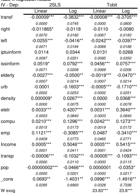
Table 4: Regression Results
IV - Dep: 2SLS Tobit
Linear Log Linear Log
transf -0.00009*** -0.3832*** -0.00008*** -0.3705***
0.0000 0.0745 0.0000 0.0800
right -0.011865* -0.0118 -0.0110 -0.0080
0.0070 0.0182 0.0067 0.0183
left -0.0255*** -0.0416** -0.0242*** -0.0397**
0.0071 0.0184 0.0069 0.0188
iptuinform 0.0114 0.0344 0.0131 0.0268
0.0097 0.0351 0.0095 0.0350
issinform 0.0519* 0.0792*** 0.0456*** 0.0757***
0.0071 0.0208 0.0069 0.0206
elderly -0.0027*** -0.0500** -0.0019*** -0.0470**
0.0007 0.0214 0.0007 0.0214
urb -0.0001 -0.1603*** -0.0005*** -0.1710***
0.0002 0.0253 0.0002 0.0251
density 0.000009* 0.0267*** 0.0000 0.0368***
0.0000 0.0075 0.0000 0.0078
eletr 0.0033*** 0.4207*** 0.0031*** 0.3640***
0.0003 0.0840 0.0003 0.0840
compu 0.0210*** 0.1296*** 0.0242*** 0.1273***
0.0015 0.0173 0.0019 0.0172
emp 0.1121*** -0.3085*** 0.0487 -0.3410***
0.0409 0.0773 0.0465 0.0771
Income 0.0005*** 0.5046*** 0.0005*** 0.5415***
0.0001 0.0411 0.0001 0.0424
transp -0.00006*** -0.1032*** -0.00005*** -0.1093***
0.0000 0.0110 0.0000 0.0115
pop -0.00000002*** -0.0466*** 0.0000001 -0.0353*
0.0000 0.0201 0.0000 0.0217
_cons 0.0693** -1.4031** 0.0996*** -1.4916**
0.0295 0.6993 0.0328 0.7336
W exog 23.83*** 23.8***
***, **, * signific. at 1%, 5% and 10%.
Standard errors in italics
The results suggest that intergovernmental transfers have a negative and statistically
significant impact on the efficiency score in tax collection. This leads to a reinterpretation of the
flypaper effect, i,e, the higher the level of transfers to the municipalities, the lower incentives they
have to increase the efficiency in tax collection. In other words, weighting for the cost of tax
collection (the inputs are capital and labor, defined in the FDH section), transfers causes a reduction
in tax collection. In particular, One can note that for $1 of additional transfer we have a decrease in
efficiency scores from 0,00009 (linear) to 0,38 (log).This means that intergovernmental transfers lead
municipality. This reinforces Dougan and Kenyon (1988) ´s argument since the interest groups which
benefit with those transfers might reduce their lobby efforts, leading in turn to a decrease in the tax
collection effort of the municipalities. Income has a positive and statistically significant effect on the
efficiency score as expected, and also a smaller magnitude in absolute terms as suggested by our
model.
Interestingly, this result holds when we consider both the linear and the logarithmic versions of
the model . Becker´s (1996) intuition can only be observed when the amount of tax revenue is the
only output . This seems to be reasonable because in this case we have a dependent variable that we
can take as equivalent to local expenditures in equilibrium (see appendix for this result). However, we
dispute that the objective of tax collection is exclusively tax revenues. It should also include how the
available tax bases are being taxed. In this case, when both are included as tax collection outputs, then
our results are robust to model specifications.
Most of control variables are statistically significant and have the expected sign.
Comparative advanced systems of tax collection are associated positively with efficiency
scores. The exception is the electronic property tax data set (IPTUinform) that it is not statistically
significant. The electronic tax collection can help the local government to interact with higher spheres
of the government when auditing individuals when a tax on services is under consideration (there is a
high degree of informality in the provision of services) but the same does not have to be true for a tax
on property.
Left wing governments are in general less efficient as expected since they tend to collect higher
revenues from a smaller size of government.
Concerning the pressure groups, the sign of the coefficients are also according to our
expectations. The lobby of elderly, for instance, influences negatively the tax collection efficiency,
that is, they reduce the tax effort as well as people that live in urban areas. Since they usually claim
for exemption local governments can reduce the number of workers allocated to auditing, or to
decrease investments that can help in tax collection.
4. Conclusions
The purpose of this paper is to propose a reinterpretation of the traditional flypaper effect
according to which central government transfers to local governments increase public spending
(taxation) more than do increases in private income. Here higher transfers from the federal
government might induce less efficiency in local tax collection.
We initially develop a simple theoretical model where the revisited flypaper effect is derived.
We then try to verify empirically if the theoretical result is empirically plausible, estimating the
flypaper effect on tax collection efficiency for Brazilian municipalities in 2004. In particular,
applying a non-parametric methodology - FDH (Free Disposable Hull), we construct efficiency scores
in tax collection for each municipality, taking into consideration two outputs: amount of per capita
17
eliminates the price- effect of tax collection, since it captures its extension taking into consideration
the associated cost of tax imposition and/or auditing. Second, we build an exogenous instrument for
intergovernmental transfers from the rules established on the Brazilian Constitution in 1988 to
transfer unconditional funds to municipalities. The idea is to eliminate the endogenous characteristic
of intergovernmental transfers due to political factors, as described above. Our results suggest that
unconditional grants affect negatively the efficiency in tax collection, leading to a reinterpretation of
the flypaper effect.
Another interesting result links interest groups (represented by the elderly, the employed, and the
urban population) to inefficiency in tax collection. The higher the percentage of people over 65 , the
smaller the level of tax revenue, and the higher the inefficiency, since they are usually exempted of
municipality tax in Brazil. The higher the percentage of people employed and the higher the degree of
urbanization, the easier is to collect taxes. Therefore, we would expect to observe a positive
relationship between these variables and tax potential. However, the urban and the employed
population do not want to be fiscally penalized and pressure for exemptions, for a greater fiscal effort
on the agricultural sector, and a decrease in informality. That is why we observe an inverse
relationship between these variables and tax potential and efficiency.
One lesson that comes from our results is that local governments in Brazil should seek additional
revenues from their own resources. This does not mean though to implement any new taxes, but to
exploit more efficiently the existing tax base. If the result obtained here, and the lesson that comes out
of it, is general enough is a question open to further investigation. In other federations besides Brazil,
the municipalities depend a lot on transfers to guarantee the provision of public goods and services
since the local tax bases are small. Following the traditional literature on the flypaper effect grant
receipts and taxes can only be equivalent resources theoretically, but we will only know if we look
carefully at other fiscally decentralized economies.
Appendix
A.1. FDH Methodology
Therefore, to determine the efficiency scores using FDH analysis, we assume n
municipalities, m products/services produced by those governments with k inputs. In terms of
production function
(1)
where
y
mx1 is the output vector andx
kx1 corresponds to the input vector. One can rank themunicipality i if it is not the most efficient in terms of input
(2)
) (
) (
,...., 1 ,....,
1
i x
n x MAX
MINi=n nl j= m j
n
i
x
F
and
n
1,...,
n
l are l municipalities more efficient than municipality i.Similarly, in terms of output, municipality i can be ranked in relation to the most efficient
(3)
The procedure can be summarized as follows. First a producer is selected. Then all producers
that are more efficient than it are marked. For every pair of producers containing the unit under
analysis and the more efficient one is computed a score for each input (dividing the input of the unit
under analysis and the more efficient one). Then select the more efficient producer that brings the unit
under analysis closest to the frontier. The calculation of the input efficiency score can be illustrated
with an example, Suppose 3 producers with a 2-input 2-output case, A (20, 33; 15, 10), B(19, 30,
16,12), C(25, 32 ; 16, 11). The first two numbers denotes inputs while the last two numbers yield
outputs. A is less efficient than B -A uses more of both inputs while its outputs is smaller. However, C
is not more efficient than A. The input score for A can be calculated in the table below. Observe that
since C is not compared to neither A and B, it gets score equal to 1. B also receives 1 because it is
more efficient than A and there is no other municipality more efficient than it is.i
Table 1A – Example
A2. Data descritption
Table 2A. Description of variables
Description Variable Name Search
The parties classified as center-left and left are denominated by the variable left and the parties from center-right and right are denoted as right. Dummy variable equal 1 for parties classified left (right) and zero the
otherwise. Left and Right
We use the ideological classification of the parties of the mayors for 2004 (Pesquisa de Informações Básicas Municipais of the IBGE) following the classification proposed by Coppedge (1997) Dummy variable equals 1 whether the
municipality has the tax service data set computerized and zero the otherwise.
IPTUinform and ISSinform
Pesquisa de Informações Básicas Municipais, IBGE,
2004 The percentage of people with more than
sixty five years in the municipality living
alone. Elderly Ipeadata, 2000.
The percentage of urban population over
resident population in the municipality. Urb Ipeadata, 2000.
The population density in the municipality Density Ipeadata, 2000 The percentage of people in the municipality
with electric energy in their residence. Eletr Ipeadata, 2000
The percentage of residents in the Comp Ipeadata, 2000
) (
) (
,...., 1 ,....,
1
i y
n y MIN
MAX
j j m j nl n
municipality with a computer in their residence.
The Economically Active Population divided
by the Working Age Population. Emp Ipeadata, 2000
The cost of transport of the Municipal Headquarters until the nearest State Capital.
Transp
Ipeadata, 1995 The percentage of population in the
municipality divided by the state population.
Pop
Ipeadata, 2000 The transfers per capita of both the state and
municipal governments.
Transf
Ipeadata, 2004 The income per capita in the municipality. Income Ipeadata, 2004
A.3. Estimation results – First Stage.
Table 3A: First Stage Regression First Stage - Dependent transf
Linear Log Linear Log
Transftab 1,091 *** 0.397***
25.033 0.038
right -23.858 -0.018 -5.009 0.013
15.403 0.014 19.308 0.013
left -40.164** 0.005 -21.156 0.022*
15.792 0.013 19.796 0.014
iptuinform 8.850 -0.023* -37.002 -0.017
21.531 0.013 26.968 0.019
issinform 31.431** 0.017* -39.482** 0.015
15.775 0.011 19.677 0.014
elderly 0.607 -0.036*** 4.457** -0.053***
1.597 0.012 2.000 0.015
urb -1.128*** -0.037*** -5.434*** -0.045***
0.381 0.013 0.462 0.015
density -0.021* -0.025*** -0.016 -0.018***
0.012 0.006 0.015 0.005
eletr 1.278** 0.031 8.354*** 0.082**
0.631 0.037 0.765 0.040
compu -6.645** 0.013* -33.005*** 0.021**
3.273 0.007 4.034 0.009
emp -15.128 -0.061* 30.802 -0.098**
90.463 0.034 113.432 0.045
Income 1.153*** 0.257*** 1.969*** 0.253***
0.149 0.020 0.186 0.022
transp 0.062*** -0.005 0.155*** -0.023***
0.018 0.009 0.022 0.009
pop -0.00004* -0.070*** -0.00007** -0.275***
0.000 0.019 0.000 0.006
_cons 145.68** 6.605*** 83.148 7.972***
65.333 0.205 81.907 0.222
***, **, * significants at 1%, 5% and 10% respectively
Adj R2 0.4598 0.602 0.155 0.552
Standard errors in italics.
Table 4A: Regression Results for the two outputs separately
IV - Dep: Tax revenue Proportion of informal workers - Tax Base
2SLS Tobit 2SLS Tobit
Linear Log Linear Log Linear Log Linear Log
transf -0.00002*** 0.1326 -0.00003**0.1707 -0,0001*** -0,497*** -0.0001*** -0.4884***
0.0000 0.1318 0.0000 0.1419 0.0000 0.0821 0.0000 0.0850
right 0.0006 0.0142 -0.0039 0.0202 -0,0118* -0.0044 -0.0108 -0.0056
0.0053 0.0312 0.0043 0.0313 0.0070 0.0203 0.0069 0.0204
left 0.0153*** 0.0267 0.0111** 0.0305 -0,026*** -0,0401* -0.0252*** -0.0388*
0.0056 0.0317 0.0047 0.0319 0.0072 0.0207 0.0071 0.0207
iptuinform -0.0151*** -0.0539 -0.0130*** -0.0694 0.0138 0.044 0.0170* 0.0345
0.0057 0.0547 0.0049 0.0537 0.0097 0.038 0.0094 0.0374
issinform 0.0064* 0.0842** 0.0076** 0.0779** 0,0532* 0,0860*** 0.0523*** 0.0848***
0.0040 0.0336 0.0033 0.0337 0.0071 0.0228 0.0070 0.0228
elderly 0.0014** 0.1312*** 0.0020*** 0.1375*** -0,0034*** -0,0708*** -0.0030*** -0.0698
0.0006 0.0350 0.0005 0.0350 0.0007 0.0234 0.0007 0.0233
urb 0.00067*** 0.1072*** 0.0004*** 0.1068*** -0.0002 -0,1872*** -0.0003*** -0.1879***
0.0001 0.0396 0.0001 0.0395 0.0002 0.0269 0.0002 0.0271
density 0.00004*** -0.0167 0.00002* -0.0110 0.0000 0,0327*** 0.000005 0.0346***
0.0000 0.0135 0.0000 0.0138 0.0000 0.008 0.0000 0.0081
eletr -0.0012*** -0.3466*** -0.0009*** -0.3609*** 0,0036*** 0,5165*** 0.0036*** 0.5041***
0.0002 0.1180 0.0002 0.1182 0.0003 0.0911 0.0003 0.0910
compu 0.0138*** 0.0268 0.0121*** 0.0214 0,0200*** 0,1354*** 0.0207*** 0.1376***
0.0016 0.0241 0.0014 0.0241 0.0018 0.0187 0.0017 0.0185
emp 0.0003*** 0.8931*** -0.0603*** -0.3048*** 0,0004*** 0,5132*** 0.1208** -0.3443***
0.0001 0.0639 0.0225 0.1115 0.0001 0.0459 0.0481 0.0835
Income -0.0643** -0.3035*** 0.0003*** 0.9050*** 0,1319*** -0,3319** 0.0004*** 0.5146***
0.0260 0.1117 0.0000 0.0656 0.0485 0.0849 0.0001 0.0463
transp -0.00003*** -0.1415*** -0.00002** -0.1406*** -0,00005*** -0,0972*** -0.00005** -0.0995***
0.0000 0.0207 0.0000 0.0210 0.00001 0.0118 0.0000 0.0119
pop 0.0000 0.2807*** 0.0000001*0.2980*** -0,00000002 -0,0668*** -0.0000000 -0.0633***
0.0000 0.0373 0.0000 0.0403 0.0000 0.0216 0.0000 0.0226
_cons 0.1259*** -9.2634*** 0.1033*** -9.6888*** 0.0513 -0.9182 0.0479 -0.9473
0.0202 1.2398 0.0175 1.3086 0.0339 0.7691 0.0335 0.7888
W exog 17.24*** 2.36* 26.4*** 24.7***
***, **, * signific. at 1%, 5% and 10%. Standard errors in italics
References
Afonso, A. and Aubyn, M.S. (2004) Non-parametric Approaches to Education and Health expenditure
Efficiency in OECD countries. Working Paper, Technical University of Lisbon.
Alfirman, L. (2003) Estimating stochastic frontier tax potential: Can Indonesian local governments
increase tax revenues under decentralization? Working Paper 03-19. University of Colorado at
Boulder, 2003.
Bailey. S. and Connolly, S. (1998). The flypaper effect: identifying areas for further research. Public
Choice, 95: 335-361.
Bajada C. (2002) How Reliable are Estimates of the Underground Economy? Economics Bulletin, Vol.
3, No. 14 pp. 1-11.
Baron, D. P. and Ferejohn, J.A. (1987) Bargaining and Agenda Formation in Legislatures. The
American Economic Review, 77(2):303-309.
Baron, D. P. and Ferejohn, J.A. (1989) Bargaining in Legislatures. American Political Science Review,
Becker, E.(1996). The illusion of fiscal illusion: Unsticking the flypaper effect. Public Choice, 86:
85-102.
Becker, G. (1983) A theory of competition among pressure groups for political influence. Quarterly
Journal of Economics, August: 371-400.
Blundell, R., Duncan, a. and Meghir, C. (1998), Estimating Labor supply responses using tax reforms,
Econometrica, p. 243-249.
Coppedge, M. (1997). A Classification of Latin American Political Parties. The Helen Kellogg Institute
for International Studies, Working Paper Series # 244.
(http://www.nd.edu/%7Ekellogg/WPS/244.pdf)
Courant, P. N. , Gramlich E.M. and Rubinfield, D. (1979) The stimulative effects of intergovernmental
grants, or Why Money sticks where it hits. In Fiscal Federalism and Grants-in-Aid, edited by
Mieszkowski and Oakland. Washington. Urban Institute.
Deprins, D., Simar, L. and Tulkens H. (1984), Measuring labor-efficiency in post-offices. In: M.
Marchand, P. Pestiau and H. Tulkens (Eds), The performance of public enterprises: concepts
and measurement. Amsterdan: North Holand.
Dougan, W.R. and Kenyon, D.A. (1988). Pressure groups and public expenditure: the flypaper effect
reconsidered. Economic Inquiry, XXVI: 159-170.
Feldstein, M.S. (1975). Wealth neutrality and local choice in public education. American Econmic
Review 65: 75-89.
Filimon, R., Romer, T. and Rosenthal, H. (1982) Asymetric information and agenda control. Journal
of Public Economics, February: 51-70.
Fisher, R.C. (1982) Income and Grants Effects on Local Expenditure: The flypaper effect and other
difficults. Journal of Public Economics, 17:15:58
Giles, D.E. and Caragata, P.J. (1998). The learning Path of the Hidden Economy: Tax and growth
effects in New Zealand. Department of Economics, University of Victoria. Government
Finance Statistics Yearbook, 1993 International Monetary Fund.
Gordon, N. (2004) Do federal grants boost school spending? Evidence from Title I, Journal of Public
Economics 88(9-10): 1771-92.
Gramlich, E.M. (1977). Intergovernmental Grants: A Review of the Empirical Literature, in W.E.
Oates, The Political Economy of Fiscal Federalism, AGPS, Canderra.
Gupta, S. and Verhoeven, M. (2001), The efficiency of government expenditure. Experiences from
Africa. Journal of Policy Modelling, 23, 433 - 467.
Greene, W. H. (2003). Econometric Analysis. Prentice Hall. Fifth Edition.
Grossman, P.J. (1994) A political theory of intergovernmental grants. Public Choice, 78: 295-303.
Hausman, J. and Poterba, P. (1987), Household behavior and the tax reform act of 1986, Journal of