GenomeFingerprinter: the genome fingerprint and the universal genome fingerprint analysis for systematic comparative genomics.

(1)

Universal Genome Fingerprint Analysis for Systematic

Comparative Genomics

Yuncan Ai1,2*, Hannan Ai1, Fanmei Meng1, Lei Zhao1

1State Key Laboratory for Biocontrol, School of Life Sciences, Sun Yat-sen University, Guangzhou, P. R. China,2Allergy Research Branch, State Key Laboratory of

Respiratory Disease, The Second Affiliated Hospital, Guangzhou Medical University, Guangzhou, P. R. China

Abstract

Background:No attention has been paid on comparing a set of genome sequences crossing genetic components and biological categories with far divergence over large size range. We define it as the systematic comparative genomics and aim to develop the methodology.

Results:First, we create a method,GenomeFingerprinter, to unambiguously produce a set of three-dimensional coordinates from a sequence, followed by one three-dimensional plot and six two-dimensional trajectory projections, to illustrate the genome fingerprint of a given genome sequence. Second, we develop a set of concepts and tools, and thereby establish a method called the universal genome fingerprint analysis (UGFA). Particularly, we define the total genetic component configuration (TGCC) (including chromosome, plasmid, and phage) for describing a strain as a systematic unit, the universal genome fingerprint map (UGFM) of TGCC for differentiating strains as a universal system, and the systematic comparative genomics (SCG) for comparing a set of genomes crossing genetic components and biological categories. Third, we construct a method of quantitative analysis to compare two genomes by using the outcome dataset of genome fingerprint analysis. Specifically, we define the geometric center and its geometric mean for a given genome fingerprint map, followed by the Euclidean distance, the differentiate rate, and the weighted differentiate rate to quantitatively describe the difference between two genomes of comparison. Moreover, we demonstrate the applications through case studies on various genome sequences, giving tremendous insights into the critical issues in microbial genomics and taxonomy.

Conclusions:We have created a method,GenomeFingerprinter, for rapidly computing, geometrically visualizing, intuitively comparing a set of genomes at genome fingerprint level, and hence established a method called the universal genome fingerprint analysis, as well as developed a method of quantitative analysis of the outcome dataset. These have set up the methodology of systematic comparative genomics based on the genome fingerprint analysis.

Citation:Ai Y, Ai H, Meng F, Zhao L (2013)GenomeFingerprinter: The Genome Fingerprint and the Universal Genome Fingerprint Analysis for Systematic Comparative Genomics. PLoS ONE 8(10): e77912. doi:10.1371/journal.pone.0077912

Editor:Vladimir Brusic, Dana-Farber Cancer Institute, United States of America ReceivedMarch 8, 2013;AcceptedSeptember 5, 2013;PublishedOctober 29, 2013

Copyright:ß2013 Ai et al. This is an open-access article distributed under the terms of the Creative Commons Attribution License, which permits unrestricted use, distribution, and reproduction in any medium, provided the original author and source are credited.

Funding:This work was supported in part by the grants to YA from the National High Technology Research & Development Project (863 Project) (No. 2006AA09Z420), National Science and Technology Major Project of China (No. 2014ZX0801105B002). HA was a recipient of the Guangzhou Municipal Science Ambassador Scholarship. The funders had no role in study design, data collection and analysis, decision to publish, or preparation of the manuscript. Competing Interests:The authors have declared that no competing interests exist.

* E-mail: Lssayc@mail.sysu.edu.cn

Introduction

By using conventional methods based on pair-wisely base-to-base comparison, comparing whole-genome sequences at large scale has not been achieved; even no attention was paid on handling a number of genomes crossing genetic components (chromosomes, plasmids, and phages) and biological categories (bacteria, archaeal bacteria, and viruses) with far divergence over large size range. We define such comparisons as the systematic comparative genomics. We believe it should be a priority task to carry out whole-genome-wide comparative genomics at large scale based on the geometrical analysis of sequences crossing diverse genetic components and biological categories in the post-genomic era. However, even simply visualizing a DNA sequence has been challenging for decades; little progress has been made to date [1].

Pioneering works in geometrical visualizing DNA sequences using computers had been done in one-dimension [2,3], two-dimensions (Z-curve) [4], and three-two-dimensions (H-curve) [5,6]. However, those were valid only for ‘static’ modeling and visualizing. The ‘dynamic’ modeling and visualizing had been explored in a virtual reality environment [7,8]. AND-viewer, for example, provided a three-dimensional sensing of a big picture of a DNA sequence in a virtual reality environment by using a hand-sensor instead of mouse and keyboard [7,8]. This pioneering work made fantastic progress in dynamically mimicking 3D visions and intuitively sensing genome sequences [7,8]. Still, there was no possibility of using the outcome dataset to further explore the real contexts of biology.

(2)

small scale. These methods were divided into two types: algebraic approach [9,10,11,12] and geometrical approach [13].

The algebraic approach means that the calculation of similarity or identity is based on pair-wisely base-to-base comparison. The output dataset is only used for visualization through graphical techniques [1]. The most common tools were BLAST [9] and CLUSTALW [10]. Recently, a BLAST-based tool, BRIG, was constructed for genome-wide comparison to create images of multiple circular genomes among a number of very closely related bacteria strains [11]. The output image showed the BLAST-similarity between one central reference sequence and other inquiry sequences as a set of concentric rings, in which BLAST-matches were colored on a sliding scale indicating a defined percentage of BLAST-identity. This tool had great advantages over other common tools, like ACT [12], in terms of the numbers of genomes being simultaneously compared and the ways of presenting its output images. These features made it a versatile tool for visualizing a range of genome data, but it was still only for visualization. Similarly, the Mauve program [14,15], combining both algebraic calculation and graphic display, was widely used for comparing and visualizing a set of genomes. However, even within close relatives, the number of genomes being handled by Mauve was dramatically dependent on the computational constraints, taking up too much CPU time or causing memory overflow, which limited Mauve to handle few very close relatives at one time.

The geometrical approach means that a genome sequence can be transformed into a set of coordinates to be plotted giving a geometrical vision. Most importantly, both calculation and visualization are separately processed in a dynamic way so that the input and output can be subsequently re-useable for geometrical analysis. One promising example was the Z-curve method (Zplotter program), which generated a set of three-dimensional coordinates from a linear genome sequence [16]. Such coordinates were plotted to create three-dimensional geometrical visions (as open rough Z-curves) for the given DNA sequences [16]. Hundreds of such visions for microbial genomes were collected as a database [17]. The Z-curve method (Zplotter program) was used not only for visualization but for geometrical analysis to explore the real contexts of biology [18,19,20,21]. For example, two replicationoripoints in archaeal bacterial genomes were predicted by the Z-curve analysis [22,23] and confirmed by the wet experiments in other labs [24,25], thus showing it’s promising. However, the Zplotter algorithm had an inevitable flaw to falsely present a genome sequence due to its ambiguous cutting-point error (see Discussion section), which was not be suitable for creating a stable unique genome fingerprint, as we proposed; nonetheless, no statistic analysis could be further applied to the outcome dataset.

In this paper, we present a method calledGenomeFingerprinterto unambiguously produce a unique set of three-dimensional coordinates from a sequence, followed by one three-dimensional plot and six two-dimensional trajectory projections, to illustrate the whole-genome fingerprint of a given genome sequence. We further develop a set of concepts and tools, and thereby establish a method called the universal genome fingerprint analysis (UGFA). Finally, we construct a method to quantitatively analyze the outcome dataset of genome fingerprint analysis. Moreover, we demonstrate the applications of such methods through various case studies, giving new insights into the critical issues in microbial genomics and taxonomy. These have set up the methodology of what we called the systematic comparative genomics based on the genome fingerprint and the universal genome fingerprint analysis. We anticipate that these comprehensive methods can be widely applied at large scale in the post-genomic era.

Results

1. Mathematical Model and Three-dimensional Coordinate

To geometrically visualize a sequence, the key step is to create a set of three-dimensional coordinates (xn, yn, zn) for each base. To

do this, the Z-curve method (Zplotter program) [16] defined a set of coordinates (xn, yn, zn) for each base in a linear sequence (n = 1,

2, …, N; N is the sequence length) by the equation (0), which defined a unique Z-curve for a given linear sequence andvice versa. Note that An, Tn, Gn, Cnwere the sum of total numbers of each of

four base-type (A, T, G, C), respectively, counting from the first base to the bases before the first base (passing through the nthbase in the process) in a linear sequence (n = 1, 2, …, N). However, the main problem was the ambiguity of the ‘‘first base’’ due to cutting-point error in a deposited sequence (see explanations in Discussion section).

xn~(AnzGn){(CnzTn)

yn~(AnzCn){(GnzTn)

zn~(AnzTn){(CnzGn)

8 > <

> :

, (n~1,2,:::,N) ð0Þ

Here we take the same defining form as the equation (0), but with different contents of An, Tn, Gn, Cn. Namely, we propose a

model calledGenomeFingerprinterfor the geometrical visualization of a circular sequence. As an artificial example, a circular sequence containing 40-bps, (59-39) ACACTGACGCACACTGACGCA-CACTGACGCACACTGACGC (Figure 1), will be used to illustrate the conceptual framework. It will be described in reasonable detail in order to build a bridge for the readers who may not have multiple disciplinary backgrounds [26].

First, we randomly select a base (the nth) as the first targeted base (TB) while keep the mthfocusing base (FB) moving. We define the relative distance (RD) (1) between the selected TB (nth) and the moving FB (mth) (m = 1, 2, …, N).

RDm n~

1, (m~nz1) 2, (m~nz2)

::: :::

N{1, (m~_nz_n{1)

N, (m~nzn) 8 > > > > > > < > > > > > > :

, (n~1,2,_:::,N) ð1Þ

Note that the RD concept is extremely critical. The RD formula (1) can virtually treat an arbitrary linear sequence as a circular one. For example, once we select the TB (e.g., suppose at position 1, baseA) and the moving FB (e.g., suppose at position 20, baseC), the RD value is 19 (Figure 1). Thus, a collection of RD values (m = 1, 2, …, N) can be generated for each selected TB (in total N number) sliding along with the given sequence. Particularly, the RD value is N, not zero, when the mthFB is located at the same position with TB, which means the mthFB has gone through one circle (i.e., starting from and finishing at the same position at the nthbase).

(3)

WRDm n~

RDm n

N , (n~1,2,:::,N) ð2Þ

Third, for the same selected TB (nth), we define the sum of the weighted relative distance (SWRD) (3) from the collection of WRD (m = 1, 2, …, N) for each of four base-type (A, G, T, C), respectively.

SWRDA n~

PA

n(WRDmn)

SWRDG n~

PG

n(WRDmn)

SWRDT n~

PT

n(WRDmn)

SWRDC n~

PC

n(WRDmn)

8 > > > > < > > > > :

, (m~1,2,:::,N) ð3Þ

Fourth, we define a set of coordinates (xn, yn, zn) (4) for the

selected TB (nth). Note that we count the sum of the weighted relative distance (SWRD) (unlike the Zplotter program counting the sum of numbers) for each of four base-type (A, T, G, C), respectively. So far, only one cycle has been done for only one selected TB (nth); namely, only one base has had its coordinates (xn, yn, zn).

xn~(SWRDA

nzSWRDGn){(SWRDCnzSWRDTn) yn~(SWRDA

nzSWRDCn){(SWRDGnzSWRDTn) zn~(SWRDA

nzSWRDTn){(SWRDCnzSWRDGn) 8

> <

> :

, (n~1,2,:::,N)ð4Þ

Finally, we repeat the above steps to create a set of coordinates for every base in the sequence. Briefly, by selecting the next TB (e.g., n = 2) and reiterating the processes for each base, step-by-step, we will finish the N cycles (n = 1, 2, …, N); and each cycle has one selected TB, which will create one set of coordinates (xn, yn,

zn) for that chosen TB. Ultimately, after having finished the total N

cycles, all N bases of the sequence will have their own coordinates so that a series of sets of coordinates (xn, yn, zn) will be created for

the genome sequence. We have developed an in-house script, GenomeFingerprinter.exe to do all. Note that our method is also valid for RNA by simply replacing T with U base.

As an example, by using our program GenomeFingerprinter.-exe, we can calculate a series of coordinates (xn, yn, zn) for the

artificial genome sequence containing 40-bps (Figure 1); there are total 40 bases and each base has its own coordinates (xn, yn, zn)

(data not shown).

2. Three-dimensional Plot and the Primary Genome Fingerprint Map

The set of coordinates (xn, yn, zn) of a given sequence can be

plotted as a three-dimensional plot (3D-P) to give a geometrical vision. As an example, the artificial sequence (Figure 1) has only 40 points giving a naive vision (not shown). Instead, we show the real visions of strains from bacteria and archaeal bacteria (Table 1) (Figure 2). Clearly, each vision (Figure 2) has its individual genome fingerprint (GF). We define such a GF vision as the genome fingerprint map (GFM), which is an intuitive identity or a unique digital marker for a given genome sequence. For convenience, we further define such a GFM vision of three-dimensional plot as the primary genome fingerprint map (P-GFM). Therefore, from now on, we can directly operate and compare the GFM vision for comparing sequences. In other words, we compare genome sequences through the genome fingerprints (via geometrical analysis) instead of the sequence base-pairs (via algebraic analysis). For instance, we can intuitively distinguish a number of genome sequences based on their genome fingerprint maps (Figure 2). Within the same speciesSulfolobus islandicus, strains M.14.25 and M.16.4 share similarity (Figure 2, A), indicating subtle variations at strain level. With far divergence, however, strain S. islandicus

Y.N.15.51 differs globally fromMethanococcus voltaeA3 but shares local similar regions (Figure 2, B); whereasS. islandicusY.G.57.14 completely differs from Methanosphaera stadtmanae DSM 3091 (Figure 2, C), confirming their farther divergences beyond genus level.

3. Two-dimensional Trajectory Projections and the Secondary Genome Fingerprint Maps

To demonstrate the genome fingerprint in a more sophisticated way, we further create six two-dimensional trajectory projections (2D-TPs) for a given P-GFM through six combinations (xn,n,

yn,n, zn,n, xn,yn, xn,zn, and yn,zn) of the coordinates. For

convenience, such six 2D-TPs are defined as the secondary genome fingerprint maps (S-GFMs). For example, the six S-GFMs comparing two chromosomes between Halobacterium sp. NRC-1 (NC_002607) andHalobacterium salinarumR1 (NC_010364) clearly demonstrate the subtle variations both globally and locally (Figure 3). Note that the S-GFMs of xn,zn, yn,zn, xn,ynusually

Figure 1. A mathematical model for creating a set of coordinates (xn, yn, zn) from a circular genome sequence.We randomly select a base (the nth_{) as the first target base (TB) while keep} moving the mth_{focusing base (FB). For the given TB (n}th_{), we define the} relative distance (RD) between the selected TB (nth_{) and the moving FB} (mth) (m = 1, 2, …, N).

doi:10.1371/journal.pone.0077912.g001

(4)

Table 1.Features of genome sequences from bacteria and archaeal bacteria.

Species and Strain Sequence ID Type Size (bps)

Downloaded from FTP.ncbi.nlm.nih.gov [GenBank]

Escherichia coliK-12/W3110 AC_000091

NC_007779

Chromosome 4646332

Escherichia coliK-12/DH10B NC_010473 Chromosome 4686137

Escherichia coliK-12/MG1655 NC_000913 Chromosome 4639675

Escherichia coliBL21 (DE3) pLysSAG NC_012947 Chromosome 4570938

Escherichia coliO55:H7/CB9615 NC_013941 Chromosome 5386352

Escherichia coliUTI89 NC_007946 Chromosome 5065741

Escherichia coliCFT073 NC_004431 Chromosome 5231428

Escherichia coliSMS-3-5 NC_010498 Chromosome 5068389

Sulfolobus islandicusM.14.25 NC_012588 Chromosome 2608832

Sulfolobus islandicusM.16.4 NC_012726 Chromosome 2586647

Sulfolobus islandicusY.N.15.51 NC_012623 Chromosome 2812165

Sulfolobus islandicusY.G.57.14 NC_012622 Chromosome 2702058

Methanococcus voltaeA3 NC_014222 Chromosome 1936387

Methanosphaera stadtmanaeDSM 3091 NC_007681 Chromosome 1767403

Halomonas elongateDSM 2581 NC_014532 Chromosome 4119315

Halorhodospira halophiliaSL1 NC_008789 Chromosome 2716716

Halorhabdus utahensisDSM 12940 NC_013158 Chromosome 3161321

Halothermothrix oreniiH 168 NC_011899 Chromosome 2614977

Halothiobacillus neapolitanusc2 NC_013422 Chromosome 2619785

Halogeometricum boringquenseDSM 11551 NC_014729 Chromosome 2860838

Haloterrigena turkmenicaDSM 5511 NC_013743 Chromosome 3944596

Natrinema pellirubrumDSM 15624 NC_019962 Chromosome 3844629

Haloquadratum walsbyiDSM 16790 NC_008212 Chromosome 3177244

Halorubrum lacusprofundiiATCC49239 NC_012029 Chromosome 2774371

Halorubrum lacusprofundiiATCC49239 NC_012028 Chromosome 533457

Haloarcula marismortuiATCC43049 NC_006396 Chromosome 3176463

Haloarcula marismortuiATCC43049 NC_006397 Chromosome 292165

Haloarcula marismortuiATCC43049 NC_006389 plasmid pNG100 33779

Halomicrobium mukohataeiDSM 12286 NC_013202 Chromosome 3154923

Halomicrobium mukohataeiDSM 12286 NC_013201 plasmid pHmuk01 225032

Haloferax vocaniiDS2 NC_013967 Chromosome 2888440

Haloferax vocaniiDS2 NC_013964 plasmid pHV3 444162

Halobacteriumsp.NRC-1 NC_002607 Chromosome 2014239

Halobacterium salinarumR1 NC_010364 Chromosome 2000962

Derivatives created in this study [based on those sequences from GenBank]

Escherichia coliK-12/W3110-91.1.1 91.1.1 Chromosome fragment 227694

(5)

carry much more sensitive information than those of xn,n, yn,n,

and zn,n do, respectively. Accordingly, the S-GFMs can amplify

subtle variations that usually are insensitive or invisible in the P-GFMs. In particular, the S-GFMs of xn,yn, xn,znand yn,znare

much more sensitive in differentiating the local subtle variations and identifying the unique genome features; whereas the S-GFMs

of xn,n, yn,n and zn,n are relatively less informative but still

useful when focusing on global patterns (Figure 3).

4. The Universal Genome Fingerprint Map (UGFM) As shown in Figure 3, for convenience, we further define the universal genome fingerprint map (UGFM) to unify both P-GFM Table 1.Cont.

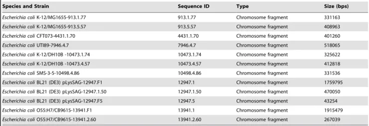
Escherichia coliK-12/MG1655-913.1.77 913.1.77 Chromosome fragment 331163

Escherichia coliK-12/MG1655-913.5.57 913.5.57 Chromosome fragment 408963

Escherichia coliCFT073-4431.1.70 4431.1.70 Chromosome fragment 401260

Escherichia coliUTI89-7946.4.7 7946.4.7 Chromosome fragment 518065

Escherichia coliK-12/DH10B -10473.1.74 10473.1.74 Chromosome fragment 325622

Escherichia coliK-12/DH10B -10473.4.57 10473.4.57 Chromosome fragment 412818

Escherichia coliSMS-3-5-10498.4.86 10498.4.86 Chromosome fragment 331536

Escherichia coliBL21 (DE3) pLysSAG-12947.F1 12947.1 Chromosome fragment 1759795

Escherichia coliBL21 (DE3) pLysSAG-12947.1.50 12947.1.50 Chromosome fragment 470050

Escherichia coliBL21 (DE3) pLysSAG-12947.F5 12947.5 Chromosome fragment 43254

Escherichia coliO55:H7/CB9615-13941.F1 13941.1 Chromosome fragment 1915479

Escherichia coliO55:H7/CB9615-13941.2.60 13941.2.60 Chromosome fragment 267039

doi:10.1371/journal.pone.0077912.t001

Figure 2. The primary genome fingerprint map (P-GFM) for the overall comparison among a number of genome fingerprint maps.

(A). Similar: Sulfolobus islandicus M.14.25 (NC_012588) and M.16.4 (NC_012726); (B). Partly similar: S. islandicus Y.N.15.51 (NC_012623) and Methanococcus voltaeA3 (NC_014222); (C). Different:S. islandicusY.G.57.14 (NC_012622) andMethanosphaera stadtmanae3091 (NC_007681); (D). Mixture: (twelve fragmental genomes of strains inEscherichia coli(listed in Table 1): 91.1.1, 91.1.61, 91.6.59, 913.1.77, 913.5.57, 4431.1.70, 7946.4.7, 10473.1.74, 10473.4.57, 10498.4.86, 12947.1.50, 13941.2.60.

(6)

(7)

and S-GFMs for the comparison in-one-sitting. Namely, we can compare a number of sequences through displaying their multiple GFMs (regardless of P-GFMs or S-GFMs) at one time (in-one-sitting) as one UGFM vision; from that, each individual GFM can be classified into a discrete group solely based on its location. For example, those P-GFMs (Figure 2, D) of the twelve fragmental genomes from eight strains of E.coli (Table 1) are enlarged and displayed on one UGFM vision, and classified into six discrete groups (Figure 4).

Clearly, there are six groups on the UGFM vision (Figure 4, A, B, C, D, E, F). Particularly, different fragmental genome sequences either from the same strain (e.g., 91.1.1, 91.1.61, 91.6.59) or from different strains (e.g., 913.5.57, 4431.1.70, 7946.4.7, 10473.1.74, 10498.4.86, 12947.1.50, 13941.2.60) (Table 1) can be revealed by the complex P-GFM patterns. Some are similar including (91.1.61, 913.1.77,10473.1.74) (Figure 4, A) and (91.6.59, 913.5.57, 13941.2.60) (Figure 4, B), but most are different (Figure 4, C, D, E, F). These data likely indicate the existence of modular domains in genomes; and such mosaic structures likely reveal their evolutionary history.

Moreover, note that a given P-GFM vision has quite different views between its own format and that of the UGFM vision (Figure 4), simply because of what we called the effects of scale-down and view-angle rotation in the UGFM vision. This feature could ensure the UGFM vision to be a powerful tool for global comparison at large scale. Namely, as many sequences as possible could be handled at one time (in-one-sitting) as long as the computer memory and the graphic software could allot.

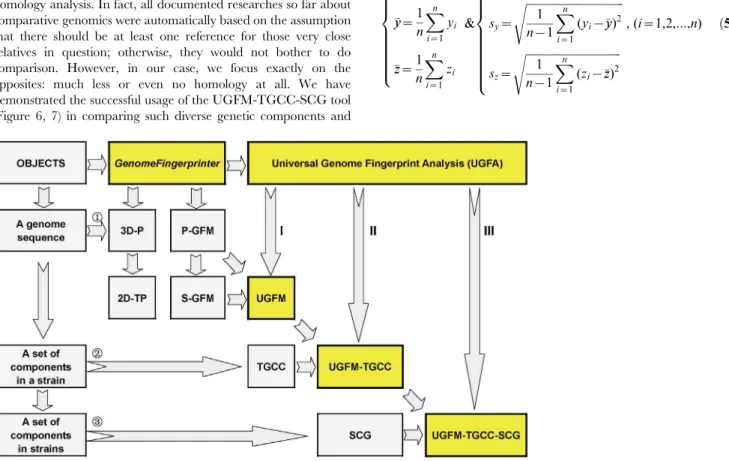
5. The Universal Genome Fingerprint Analysis (UGFA) We further establish a method called the universal genome fingerprint analysis (UGFA) (Figure 5). Briefly, the UGFA method consists of a set of concepts and tools under three subcategories corresponding to three objects: a genome, a strain, and a set of strains, respectively. In other words, the objects of comparison can be one genome sequence, a number of genome sequences crossing genetic components (chromosomes, plasmids, and phages, if applicable) in a strain, or a set of genome sequences of genetic components in strains crossing biological categories (bacteria, archaeal bacteria, viruses). We anticipate that it should be effective for what we called the systematic comparative genomics at large scale, by expanding the scope of genetic component and biological category as well as the power of computation.

5.1. UGFM. First, the UGFM tool, namely the universal genome fingerprint map (UGFM), is the foundation of the UGFA method. As shown earlier (Figure 3, 4), the UGFM (combined the P-GFM and the S-GFMs) has been proved powerful in the comparison among a number of genomes crossing both archaeal and prokaryote bacteria genomes.

5.2. UGFM-TGCC. Second, we define the total genetic component configuration (TGCC) for a set of genomes crossing genetic components (chromosomes, plasmids, and phages, if applicable) in a strain for describing the strain as a systematic unit. We further define the universal genome fingerprint map (UGFM) of the total genetic component configuration (TGCC) (UGFM-TGCC) for differentiating a set of genetic components in a strain as a universal system. Putting together, the UGFM-TGCC tool, namely the universal genome fingerprint map (UGFM) of the

total genetic component configuration (TGCC), can be used to perform the comparison among a set of genomes crossing genetic components within a strain, which will be exemplified in the next section (Figure 6).

5.3. UGFM-TGCC-SCG. Third, we define the UGFM-TGCC-SCG tool, namely UGFM-TGCC-based systematic com-parative genomics (SCG), in order to compare a set of genomes crossing both genetic components (chromosomes, plasmids, and phages, if applicable) and biological categories (bacteria, archaeal bacteria, viruses) in a universal system.

At moderate scale, one example (Figure 6) demonstrates that nineteen genomes (including six chromosomes and thirteen plasmids) with large size range (6 Kbp,4 Mbp) can be mapped

and compared by using the UGFM-TGCC-SCG tool. These nineteen genomes from four strains (each containing at least one chromosome and one plasmid) crossing four genera of halophilic Archaea (Table 1) are compared as two sets (Figure 6):Halorubrum lacusprofundiiATCC 49239 (two chromosomes and one plasmid)vs.

Haloarcula marismortuiATCC 43049 (two chromosomes and seven plasmids) (Figure 6, A, B); while Haloferax vocanii DS2 (one chromosome and four plasmids)vs.Halomicrobium mukohataeiDSM 12286 (one chromosome and one plasmid) (Figure 6, C, D). Obviously, they are shown quite divergent solely based on their genome fingerprint maps on the UGFM-TGCC-SCG visions. Most importantly, the tiny spots (e.g., corresponding to 6 Kbp) and the giant visions (e.g., corresponding to 4 Mbp) are harmoniously co-existed in the same figure, either closely or distantly.

At large scale, the UGFM-TGCC-SCG vision can demonstrate the amazing landscape of a large set of genomes both crossing diverse genetic components (chromosomes, plasmids, and phages) and crossing diverse biological categories (bacteria, archaeal bacteria, viruses). For instance, we make up a large set (over one hundred) of genomes of interest by combing 6 archaeal bacterial genomes and 13 archaeal bacterial plasmids (shown in Figure 6), 12 fragmental chromosomes ofE.coli(shown in Figure 4), 47 phage genomes and 24 virus genomes (as listed in Table 2) to be compared at large scale by using the UGFM-TGCC-SCG tool. Remind that the effects of scale-down and view-angle rotation as demonstrated earlier (Figure 4) could ensure that as many sequences as possible could be handled at one time as long as the computer memory and the graphic software could allot. Under our conditions (physical 2-Gb memory and 32-bits graphic software), we can only handle up to 1.5 Gb data in-one-sitting. As such, we generate two sets, separately. One set contains eighty three genomes: 24 viruses (I), 12 fragmental chromosomes ofE.coli

(II), and 47 phages (III), which are shown as three distinct groups (Figure 7, A). The other set consists of two archaeal bacterial chromosomes (I), two bacterial fragmental chromosomes/two phages/two viruses (II), and three plasmids (III), which are shown as three distinct groups (Figure 7, B). These are generally consistent with their real biological distinctions at different taxonomical levels. Obviously, here the effects of scale-down and view-angle rotation are demonstrated even stronger than those in earlier sections. Moreover, in the big group of phages and viruses (II), most genomes seem as very close relatives and accordingly almost repeat themselves within the phage or virus subgroup, respectively, resulting in fewer maps than should be.

Figure 3. The primary genome fingerprint map (P-GFM) (A) and the secondary genome fingerprint maps (S-GFMs) (B,H) for the

comparisons between two chromosomes ofHalobacteriumsp. NRC-1 (NC_002607) andHalobacterium salinarumR1 (NC_010364).(A). xn,yn,zn; (B). xn,yn; (C). xn,zn; (D). yn,zn; (E). xn,n; (F). yn,n; (G). zn,n; (H). xn,n and yn,n together. Note that two replicationoripoints (oriC1 andoriC2) are marked by arrows; other arrows indicated the genome-wide evolution events.

(8)

(9)

Taken together, such amazing landscapes (Figure 6, 7) can only be revealed by using the unique UGFA method, under the notions of ‘‘universal genome fingerprint map (UGFM)’’ of ‘‘total genetic component configuration (TGCC)’’ based ‘‘systematic comparative genomics (SCG)’’. Namely, these data are more than enough to prove the concepts and tools (UGFM, TGCC, and UGFM-TGCC-SCG) (Figure 5) effective and powerful in handling such real-world diverse genomes in-one-sitting. Most importantly, the representatives are elegantly plotted as beautiful and meaningful UGFM-TGCC-SCG visions (Figure 6, 7), explicitly demonstrating the scope and power of the unique comprehensive methods developed in the present study. Remarkably, we re-emphasize that the combined concept and tool of ‘‘UGFM-TGCC-SCG’’, namely the ‘‘universal genome fingerprint map (UGFM)’’ of ‘‘total genetic component configuration (TGCC)’’ based ‘‘systematic comparative genomics (SCG)’’, is distinguished from any other traditional methods of comparative genomics. This is simply because all genomes of interest crossing diverse genetic components (chromo-somes, plasmids, and phages, if applicable) and diverse biological categories (bacteria, archaeal bacteria, viruses) are much less or even no homology at all (Figure 6, 7), which should be incredibly challenging to any conventional methods based on the traditional homology analysis. In fact, all documented researches so far about comparative genomics were automatically based on the assumption that there should be at least one reference for those very close relatives in question; otherwise, they would not bother to do comparison. However, in our case, we focus exactly on the opposites: much less or even no homology at all. We have demonstrated the successful usage of the UGFM-TGCC-SCG tool (Figure 6, 7) in comparing such diverse genetic components and

diverse biological categories, regardless of the format of objects and the extent of divergences. Clearly, this is one of the core concepts and the most priority aim in the present study.

6. Quantitative Analysis of the Outcome Dataset of Genome Fingerprint Analysis

The difference between two genomes of interest, whose genome fingerprints are distinguished by one of the visions of UGFM, UGFM-TGCC, and UGFM-TGCC-SCG, can be further quan-titatively discussed as follows.

6.1. The geometric center and geometric mean of the genome fingerprint map. First, we define the geometric center (xx,yy,zz) as a unique digital indicator for its genome fingerprint map. Accordingly, the geometric center (xx,yy,zz) and the standard deviation of all coordinates (sx,sy,sz) can be

calculated (5) by GenomeFingerprinter.exe from a given genome sequence (i~1,2,:::,n) (the length of an entire genome sequence is

usually greater than hundreds of base pairs).

x x~1

n

Xn

i~1

xi

y y~1

n

Xn

i~1

yi

zz~1

n

Xn

i~1

zi 8 > > > > > > > > > > < > > > > > > > > > > : &

sx~

ffiffiffiffiffiffiffiffiffiffiffiffiffiffiffiffiffiffiffiffiffiffiffiffiffiffiffiffiffiffiffiffiffiffiffi 1

n{1 Xn

i~1 (xi{xx)2

s

sy~

ffiffiffiffiffiffiffiffiffiffiffiffiffiffiffiffiffiffiffiffiffiffiffiffiffiffiffiffiffiffiffiffiffiffiffi 1

n{1 Xn

i~1 (yi{yy)2

s

sz~

ffiffiffiffiffiffiffiffiffiffiffiffiffiffiffiffiffiffiffiffiffiffiffiffiffiffiffiffiffiffiffiffiffiffi 1

n{1 Xn

i~1 (zi{zz)2

s 8 > > > > > > > > > > > > < > > > > > > > > > > > > :

, (i~1,2,:::,n) ð5Þ

Figure 4. The universal genome fingerprint map (UGFM) for the comparison among a set of genomes in-one-sitting. Twelve fragmental genome sequences (Table 1) are shown as one UGFM vision. Each individual primary genome fingerprint map (P-GFM) is classified into a discrete group solely based on its location: Group (A) (91.1.61, 913.1.77 and 10473.1.74), Group (B) (91.6.59, 913.5.57 and 13941.2.60), Group (C) (7946.4.7 and 12947.1.50), Group (D) (10498.4.86), Group (E) (91.1.1), and Group (F) (4431.1.70).

doi:10.1371/journal.pone.0077912.g004

Figure 5. The conceptual framework of the universal genome fingerprint analysis (UGFA).The core concepts and tools include UGFM, UGFM-TGCC, and UGFM-TGCC-SCG. Abbreviations: 3D-P: three-dimensional plot; 2D-TP: two-dimensional trajectory projections; GF: genome fingerprint; GFM: genome fingerprint map; P-GFM: primary genome fingerprint map; S-GFM: secondary genome fingerprint map; UGFM: universal genome fingerprint map; TGCC: total genetic component configuration; UGFM-TGCC: universal genome fingerprint map of total genetic component configuration; SCG: systematic comparative genomics; UGFM-TGCC-SCG: universal genome fingerprint map of total genetic component configuration based systematic comparative genomics; UGFA: universal genome fingerprint analysis.

(10)

Second, we define the geometric mean (Gm) (6) of the geometric center of a given genome fingerprint map.

Gm~p3 ffiffiffiffiffiffiffiffiffiffiffiffiffiffiffiffiffi(xx)(yy)(zz) ð6Þ

Note that the definition ofGm has two-fold meanings: one is algebraically calculating the geometric-mean value of the three means (xx,yy,zz), the other is geometrically defining the side-length value of a cube that is roughly equivalent to the cuboid volume, which is created by the values of geometric center starting from and rotating around the origin in the three-dimensional space. Accordingly, the values (Gm,xx,yy,zz) are not the absolute ones but carry the symbols (minus or plus), corresponding to the geometric center of the genome fingerprint map in the same three-dimensional space, namely within the scope of geometrical analysis.

6.2. The Euclidean distance and differentiate rate between two genomes. To directly compare two genomes of interest, we define (7) the Euclidean distance (Ed), the differentiate rate (Dr%), and the weighted differentiate rate (WDr%) between two genomes in pairs, which are calculated based on the geometric means of the geometric centers of genome fingerprint maps. Again, the values (Gma,Gmb,xx,yy,zz) are not the absolute ones but

carry the symbols (minus or plus) corresponding to their geometric centers of genome fingerprint maps in the same three-dimensional space.

Ed~

ffiffiffiffiffiffiffiffiffiffiffiffiffiffiffiffiffiffiffiffiffiffiffiffiffiffiffiffiffiffiffiffiffiffiffiffiffiffiffiffiffiffiffiffiffiffiffiffiffiffiffiffiffiffiffiffiffiffiffiffiffiffiffiffiffiffi (xxa{xxb)2z(yya{yyb)2z(zza{zzb)2

q

Dr%~DGma{Gmb

GmazGmb

D|100%

WDr%~Dr%|Ed

8

> > > > <

> > > > :

ð7Þ

6.3. Examples of the quantitative comparison between two genomes. As examples, thirty chromosomes (Table 1) give twenty-nine pairs of comparison (Table 3) as the representatives for illustrating the principles. As such, the rules can be summarized from these examples (Table 3). In general, the differentiate rates (Dr%) vary from family to family; and the values ofDr%start from least at strain/species level (,50%) to higher at genus level (,500%) to even higher at beyond family level (,1500%). Of course, there are numerous outliers under certain situations (Table 3) with challenging values in terms of either the differentiate rate (Dr%), or the weighted differentiate rate (WDr%), or the Euclidean distance (Ed).

Figure 6. The UGFM-TGCC-SCG of four archaeal bacterial strains crossing four genera of halophilic Archaea.One set (A vs.B): Halorubrum lacusprofundiiATCC49239 [chromosome I (NC_012029), chromosome II (NC_012028), plasmid pHLAC01 (NC_012030)]vs.Haloarcula marismortuiATCC43049 [chromosome I (NC_006396), chromosome II (NC_006397), and seven plasmids pNG100 (NC_006389), pNG200 (NC_006390), pNG300 (NC_006391), pNG400 (NC_006392), pNG500 (NC_006393), pNG600 (NC_006394), pNG700 (NC_006395)] focusing on plasmids (A) and as a universal system (B); The other set (C vs.D): Haloferax vocanii DS2 [chromosome (NC_013967), and four plasmids pHV3 (NC_013964), pHV2 (NC_013965), pHV4 (NC_013966), pHV1 (NC_013968)] vs. Halomicrobium mukohataei DSM 12286 [chromosome (NC_013202), plasmid pHmuk01(NC_013201)] focusing on plasmids (C) and as a universal system (D). Note that the tiny spots and the giant visions are elegantly plotted in-one-sitting within the same figure.

(11)

Table 2.Features of genome sequences from phages and viruses.

Downloaded from FTP.ncbi.nlm.nih.gov [GenBank]

WA5: Coliphage WA5 NC_007847 Phage chromosome 5737

ID11: Coliphage ID11 NC_006954 Phage chromosome 5737

NC10: Coliphage NC10 NC_007854 Phage chromosome 5687

G4: Enterobacteria phage G4 NC_001420 Phage chromosome 5737

alpha3: Enterobacteria phage alpha3 DQ085810 Phage chromosome 6177

phiK: Coliphage phiK NC_001730 Phage chromosome 6263

S13: Enterobacteria phage S13 NC_001424 Phage chromosome 5540

phiX174: Coliphage phiX174 NC_001422 Phage chromosome 5540

(12)

For example, the two chromosomes of two strains (Sulfolobus islandicus M.14.25 and M.16.4) with subtle variations in their genome fingerprint maps (Figure 2, A) can be quantitatively differentiated through the distinct values of geometric center

(644.00,22081.00, 388729.15)vs.(476.50,21916.50, 387938.65) and geometric mean (28046.40)vs. (27075.85), clearly indicating they are not identical. The differentiate rate between them is only 6.42% (Table 3). Evidently, such two strains have distinct values of Table 2.Cont.

SARS coronavirusSin2679 AY283797 Virus chromosome 30132

SARS coronavirusUrbani AY278741 Virus chromosome 30153

SARS coronavirusBJ01 AY278488 Virus chromosome 30151

SARS coronavirusHKU-39849 AY278491 Virus chromosome 30168

SARS coronavirusCUHK-W1 AY278554 Virus chromosome 30162

SARS coronavirus NC_004718 Virus chromosome 30178

SARS coronavirusCUHK-Su10 AY282752 Virus chromosome 30162

Murine hepatitis virusstrain 2 AF201929 Virus chromosome 31724

Murine hepatitis virusstrain Penn 97-1 AF208066 Virus chromosome 31558

Murine hepatitis virusstrain ML-10 AF208067 Virus chromosome 31681

Murine hepatitis virusstrain A59 NC_001846 Virus chromosome 31806

Porcine epidemic diarrhea virus NC_003436 Virus chromosome 28435

Avian infectious bronchitis virus NC_001451 Virus chromosome 28004

Feline infectious peritonitis virus NC_002306 Virus chromosome 29776

Human coronavirus229E NC_002645 Virus chromosome 27709

Bovine coronavirusstrain Quebec AF220295 Virus chromosome 31546

Bovine coronavirusstrain Mebus u00735 Virus chromosome 31477

Bovine coronavirusisolate BCoV-LUN AF391542 Virus chromosome 31473

Bovine coronavirus NC_003045 Virus chromosome 31473

doi:10.1371/journal.pone.0077912.t002

Figure 7. The landscape of the UGFM-TGCC-SCG visions at large scale.(A). The twelve bacterial fragmental chromosomes ofE.coli(II) (Table 1), twenty four virus genomes (I) and forty seven phage genomes (III) (Table 2) are shown as three distinct groups, resulting in fewer maps because the genomes are very close relatives and accordingly almost repeat themselves; (B). The representatives selected from (A) are shown as three distinct groups: two archaeal bacterial chromosomes (I); two bacterial fragmental chromosomes ofE.coli, two viruses, and two phages (II); three plasmids (III). The strong effects of scale-down and view-angle rotation at large scale are demonstrated.

(13)

geometric center and geometric mean of the genome fingerprint maps, but the differentiate rate is less than 10%. Indeed, they had been characterized as two distinct but close strains within the same species,Sulfolobus islandicus. In addition, there are four close strains in this species, with differentiate rates ranging between 6.42% and 25.28% (Table 3).

Another example compares two very distant strains (beyond family level), Sulfolobus islandicus Y.G.57.14 vs. Methanosphaera stadtmanae DSM 3091 (Figure 2, C) with the following diverse data: geometric center (5251.00, 23846.00, 394896.15) vs. (4145.50, 7328.50, 395302.72), geometric mean (219979.20) vs.

(22900.28). Moreover, the differentiate rate between them is 1467.93% (Table 3), which is much greater than those values at genus level. These data together confirm that the two strains are farther divergent beyond the family level.

Furthermore, there are three remarkable exceptions (Table 3). First, within the same one strain, there are two chromosomes; and the differentiate rate between the two chromosomes is at least close

to the values between two species or genera, implying that such two chromosomes are divergent and each independently impacts on the same strain. For instance, the differentiate rates of

Halorubrum lacusprofundii49239vs. 49239-II (42.39%) andHaloarcula marismortui43049vs. 43049-II (30.68%), respectively, are close to certain values of the differentiate rates (e.g., 42.76%, 36.36%, 54.44%) at genus level within the same family Halobacteriaceae. Second, within the same species, Escherichia coli, three strains (BL21(DE3), CB9615, CFT073) are extraordinary because the differentiate rate between UT189 and BL21(DE3) is 321.11%, which is extremely out of the ranges (3.36%,36.42%) defined by

the ordinary members in the same species; and it is even much greater than the value of 25.10% between two external genera (Methanococcus voltaeA3 andMethanosphaera stadtmanae3091) in other family. Third, within the same family, Halobacteriaceae, the differentiate rates among different genera vary between 17.10% and 291.91%. Putting together, these data probably indicate that such strains (particularly containing more than one chromosome) Table 3.The quantitative analysis of representative taxa used in this study.

Taxona

x

x yy zz Gm Dr%b _WDr_%b _Edb

Escherichia coliSMS-3-5 2723.50 3286.50 225173.50 3911.76 3.36 38846.52 11544.34

Escherichia coliK-12/MG1655 2686.50 1944.50 236639.51 3657.07 6.39 3171.28 496.33 Escherichia coliK-12/DH10B 2626.50 1452.50 236613.51 3217.80 10.25 35994.85 3512.41 Escherichia coliK-12/W3110 254.00 21905.00 237151.01 2619.59 36.42 304004.04 8348.03 Escherichia coliUTI89 23518.50 1648.50 230606.51 5620.22 321.11 2987021.60 9302.08 Escherichia coliBL21 (DE3) pLysSAG 2299.00 22237.00 238421.01 22951.00 42.76 535251.30 12518.87 Escherichia coliO55:H7/CB9615 4072.00 3474.00 228174.01 27359.17 22.74 97703.92 4296.20 Escherichia coliCFT073 1205.00 3302.00 224979.00 24632.12 202.03 88805749.64 439557.42 Methanococcus voltaeA3 26408.50 2970.50 414491.71 13711.64 25.10 587771.06 23419.60 Methanosphaera stadtmanae3091 4145.50 7328.50 395302.72 22900.28 1467.93 16494288.43 11236.41 Sulfolobus islandicusY.G.57.14 5251.00 23846.00 394896.15 219979.20 19.39 451075.63 23268.54 Sulfolobus islandicusY.N.15.51 27837.50 757.50 413575.65 213490.82 25.28 667551.43 26407.22 Sulfolobus islandicusM.14.25 644.00 22081.00 388729.15 28046.40 6.42 5292.47 824.63 Sulfolobus islandicusM.16.4 476.50 21916.50 387938.65 27075.85 16.03 12422689.29 775145.76 Haloarcula marismortui43049 401.00 865.00 2387202.12 25121.13 30.68 11239486.19 366386.62 Haloarcula marismortui43049-II 21343.00 2717.00 220823.07 22716.74 216.56 73553959.06 339653.28

Halobacterium salinarumR1 2874.00 1275.00 2360470.18 7378.43 1.24 432.16 347.72

Halobacterium sp.NRC-1 2851.50 1213.50 2360811.68 7197.28 19.19 936045.35 48776.09

Halogeometricum boringquense11551 22079.00 1844.00 2312055.11 10615.71 1.58 275711.29 174157.24 Halomicrobium mukohataei12286 1900.50 21177.50 2486140.66 10284.83 42.76 2879398.22 67330.93 Halomonas elongate2581 26598.00 4630.00 2552680.14 25654.04 221.76 137405406.45 619606.27 Haloquadratum walsbyi16790 22613.00 5233.00 66913.02 29708.09 36.36 17055884.77 469043.29 Halorhabdus utahensis12940 5125.50 4368.50 2402065.63 220802.81 160.79 16003171.72 99528.02 Halorhodospira halophiliaSL1 226901.01 54859.02 2481632.18 89243.66 133.41 8899042.85 66706.24 Halorubrum lacusprofundii49239 22129.50 22139.50 2457398.67 212773.06 42.39 17797581.80 419838.30 Halorubrum lacusprofundii49239-II 21716.50 22140.50 237560.57 25167.70 54.44 31479912.34 578208.73 Haloterrigena turkmenica5511 23902.00 22238.00 2615765.16 217519.47 215.81 200314105.28 928180.28 Halothermothrix oreniiH 168 255.00 3329.00 312389.12 6424.66 291.91 126733403.82 434156.90 Halothiobacillus neapolitanusc2 2821.00 6576.00 2121748.05 213120.26 17.10 6022573.34 352284.18

Natrinema pellirubrum15624 24316.50 23111.50 2473826.67 218531.35 / / /

a_{The taxa with GenBank_ID are cross-listed in Table 1.}

b_{The Euclidean distance (}_Ed_{),differentiate rate (}_Dr_{%), and weighted differentiate rate (}_WDr_{%) are calculated according to the formula (7) by using two adjacent}

(14)

have been continuously growing and absorbing new composites so that they are potentially developing into a new species. Moreover, from family to family, the genus levels are not within the same range of divergence in terms of the differentiate rates, implying no possibility of setting up a universal boundary for simply distinguishing all taxa.

Most importantly, although the differentiate rate (Dr%) is concise and efficient for most cases (Table 3), we also note that the weighted differentiate rate (WDr%) is more accurate to deal with outliers, giving more reasonable inference through the cross-validations after having factored the differentiate rate (Dr%) with the Euclidean distance (Ed). For example, two genera ( Halogeome-tricum boringquense 11551vs. Halomicrobium mukohataei12286) seem very similar due to the tiny differentiate rate (1.58%) by chance resulting from the very similar values of Gm (10615.71 vs. 10284.83), but they are actually quite different in terms of their geometric centers (22079.00, 1844.00,2312055.11)vs. (1900.50,

21177.50,2486140.66), resulting in larger values of the weighted differentiate rate (WDr%= 275711.29) and the Euclidean distance (Ed= 174157.24), which are essentially close to the extents that distinguished the divergences between other genera in the same family. Thus, we suggest that either Dr% or WDr% can be generally referred to an inference (the first is concise while the latter is accurate); but for outliers arisen, both of them have to be cross-referenced explicitly.

Discussion

We believe that performing what we called the systematic comparative genomics based on the geometrical analysis of genome sequences, instead of the pair-wisely base-to-base com-parison, is a priority task in the post-genomic era. To our knowledge, however, no attention as what we did in the present study has been paid to compare a number of genomes crossing genetic components (chromosomes, plasmids, and phages) and biological categories (bacteria, archaeal bacteria, and viruses) with far divergence over large size range. In particular, no method for creating the unambiguous genome fingerprint (GF) has been documented; neither the universal genome fingerprint analysis (UGFA), nor the total genetic component configuration (TGCC), nor the systematic comparative genomics (SCG) has been proposed; nonetheless, no method for quantitatively differentiating genome sequences has been developed based on using the outcome dataset of genome fingerprint analysis.

Remarkably, the genome sequences crossing diverse genetic components (chromosomes, plasmids, and phages) or crossing diverse biological categories (bacteria, archaeal bacteria, and viruses) have much less or even no homology, which should be incredibly challenging to any conventional methods that are principally based on the pair-wisely base-to-base homology analysis. In other words, no conventional method can compare such diverse genetic components and biological categories in-one-sitting, as what we did in the present study. Therefore, it would be impossible to compare other conventional methods with our comprehensive methods as a whole system: the method of genome fingerprinting (GenomeFingerprinter), the method of universal genome fingerprint analysis (UGFA) (including the UGFM, UGFM-TGCC, and UGFM-TGCC-SCG tools), and the method of quantitative analysis (Gm,Ed,Dr%,WDr%) for the outcome dataset of the genome fingerprint analysis. In the present study, however, we have tried our best to compare partial features between our methods and others that are partly related to ours, as well as briefly discuss the future perspectives of quantitative

analysis for using the outcome dataset of the universal genome fingerprint analysis.

1.GenomeFingerprinter vs. Zplotter

1.1. Validity. The Zplotter program [16] is not used for the creation of what we called ‘‘genome fingerprint (GF)’’. In fact, although some coordinates from the Zplotter program were used to produce hundreds of graphs (as open rough Z-curves) of microbial genomes that were documented as a database [17], there were no stable unique features in terms of the so-called genome fingerprints. For example, when we re-plotted the visions ofHalobacteriumsp. NRC-1 genome sequence (NC_002607) using the Zplotter’s coordinates of either zn’ or zn, respectively, to

present an open rough Z-curve (data not shown), those visions themselves were quite different from one another due to the wavelet transform in the algorithm of Zplotter program [16]. In contrast, our method presented a unique circular vision with accurate and delicate genome fingerprints for the same sequence (data not shown). Again, note that using the zn, coordinates gave a

similar vision to ours, except that it was in an open rough Z-curve with less features; while using the zn’ coordinates created a

completely different vision from ours (data not shown). We conclude that our GenomeFingerprinter method provides more accurate and delicate coordinates than the Zplotter program does, and therefore is valid for the subsequent applications that have been established by the Z-curve analysis. Of course, one should beware of choosing whether zn from our method or zn’

from the Zplotter program when referring to specific questions. 1.2. Reliability. We found a major problem when using the Zplotter program to handle circular genome sequences with cutting-point errors. In fact, for example, the same circular sequence ofHalobacterium sp. NRC-1 (NC_002607) but with two different cutting-points (e.g., NC_002607_RC was re-cut at 700 kbps) were incorrectly presented as different visions by using the Zplotter’s coordinates; whereas both scenarios were exactly shown as the same vision by using our method (data not shown). The reasons for such differences come from that the Zplotter program was designed for a linear sequence [16] and its algorithm depends on counting the absolute numbers of bases starting from the ‘‘first’’ base in a given linear sequence. Meanwhile, when a sequence was deposited as a linear form (regardless of the original linear or circular form), the documented first base was usually not guaranteed to be the real first one. Taken together, the same circular sequence with cutting-point error changing its real ‘‘first’’ base can result in a quite different vision by using the Zplotter program. In contrast, our method was initially created for a circular sequence (Figure 1) but has been proved also valid for a linear one as exemplified earlier. This is not only because the linear form is a specific form of circular one, but also because the formula (1) described earlier ensures that our method measures the relative distance in a circular form, rather than the absolute numbers of bases counting from the ‘‘first’’ base in a linear sequence. In other words, our method has been proved valid for both circular and linear forms regardless of where the cutting-point is (i.e., where the ‘‘first’’ base is), overriding any possible cutting-point errors.

1.3. Adaptability. We further emphasize the scientific foundations for the reason why it is critical to deal with circular genomes, which has been overlooked in literatures.

(15)

when and only when they are at certain functioning stages of living cells, such as the rolling-model replication and the plasmid-mediated conjunction. Most importantly, the circular and linear forms are both genetically and physiologically functioning in a coordinated way for a given genome in a given living microbe. That is, their forms are interchangeable when responding to real living conditions. Therefore, we can catch up the circular status of genomes during their life cycles.

Technically, different groups world-wide have not been unified yet to guarantee that all genome sequences are deposited in their correct forms. In fact, most sequences deposited in public databases (such as GenBank) so far are neither in their natural orders of starting from the real ‘‘first’’ base, nor in the assumed direction from 59to 39. We thus have to tackle such cutting-point errors, as illustrated by those examples earlier. Fortunately, the RD formula (1) in our method can virtually treat an arbitrary linear sequence as a circular one (Figure 1), avoiding impacts of any possible cutting-point errors exist in the public deposited sequences.

Informatively, the closed (circular form) genome fingerprints carry much more sensitive information, considering genome-wide comparative genomics at the genome fingerprint level (Figure 3). Our method can precisely calculate a set of three-dimensional coordinates for a given circular or linear sequence with or without correct cutting-point, which accordingly can present a stable unique genome fingerprint map and further guarantee the validity of the universal genome fingerprint analysis.

To conclude, theGenomeFingerprinter method has great advan-tages over the Zplotter program in creating unambiguous sets of coordinates, which is valid to the subsequent applications that have been established by the Z-curve analysis [18,19,20,21,22,23].

2.Genome Fingerprinter vs. Mauve

2.1. Efficiency. The Mauve program (a typical algebraic-type approach), combining both computing and plotting, is commonly used for pair-wisely base-to-base comparison and visualization [14,15]. However, it has difficulty when dealing with a number of larger genome sequences due to its inner computational constraints, either too slow or memory overflow. In contrast, our method can rapidly calculate and visualize, separately, tens of large genomes, and is much faster than the Mauve program in terms of the time complexity [O(n)vs.O(n2) ] (data not shown). Furthermore, with our method under our hardware conditions (physical 2 Gb memory and 32-bits graphic software), more than one hundred genome sequences can be elegantly plotted in-one-sitting (Figure 7). Only plotting numerous larger graphics in-one-sitting would cause memory overflow. Most importantly, our method performs calculation and visualization separately, which not only ensures higher performance efficiency for a large set of genomes, but also provides output dataset for the universal genome fingerprint analysis (Figure 2, 3, 4, 5, 6, 7) and quantitative analysis (Table 3).

2.2. Prediction. The Mauve program [14,15] can only visualize what a sequence is, but cannot predict what it should be without one reference sequence or specific pre-knowledge. In contrast, our method provides the universal genome fingerprint map (UGFM) (either the P-GFM or the S-GFMs), which can intuitively identify the unique genome features such as the genome-wide evolution events and the replication ori points (Figure 3) that have been characterized in literatures [22,23,24,25].

2.3. Compatibility. The universal genome fingerprint anal-ysis (UGFA) predicted the subtle variations (Figure 3, C, D, G) indicating the genome-wide evolution events (Figure 3, C). We

then used the Mauve program to pair-wisely compare two chromosomes and confirmed such events (data not shown), demonstrating that the UGFA method could rapidly predict the evolution events while the Mauve program could precisely confirm such predictions. Thus, we recommend that the UGFA method and the Mauve program be compatible partners, taking advan-tages of ours for rapid intuitive prediction in general (Figure 3, 6) and of Mauve’s for slow precise confirmation in detail, particularly focusing on the targeted fragments’ gain, lose, and rearrangement (data not shown).

Likewise, among nineteen genomes (Figure 6), including six chromosomes and thirteen plasmids with large size range (6 Kbp,4 Mbp) belonging to the four strains crossing four genera of

halophilic Archaea (Table 1), the rare homology was mapped only by the progressiveMauve mode [14] (data not shown); whereas the Mauve mode [15] failed in such a comparison because it stopped due to no essential homology, as we predicted beforehand. Yet, the Mauve mode [15] worked well with the subset of either thirteen plasmids or six chromosomes, respectively, confirming their partial homology (data not shown). In other words, the UGFM-TGCC-SCG tool can not only handle the exceptional situations for a large set of genomes, but also facilitate the effective integration of the Mauve program into performing the so-called systematic compar-ative genomics among a large set of genome sequences crossing diverse genetic components (chromosomes, plasmids, and phages) and diverse biological categories (bacteria, archaeal bacteria, and viruses) with far divergence (less or no homology) over large size range (e.g., 6 Kbp,4 Mbp) (Figure 6, 7). Meanwhile, the

progressiveMauve mode [14] can be compatible to the UGFA method (including the UGFM, TGCC, and UGFM-TGCC-SCG tools), whereas the Mauve mode [15] cannot, but still can be used to partially deal with the subsets of genomes in question.

Taken together, we conclude that the UGFA method (including the UGFM, UGFM-TGCC, and UGFM-TGCC-SCG tools) has advantages over the Mauve program [14,15] in dealing with a set of genomes of less or no homology. Particularly, we recommend that any components with farther divergence be rapidly pre-screened out by using the UGFM-TGCC-SCG tool, which could guide the selection of subsets in question for the subsequent comparisons by using the appropriate mode of Mauve program [14,15].

3. The Quantitative Analysis of the Outcome Dataset of Genome Fingerprint Analysis

(16)

genus level (,500%) to even higher at beyond family level (,1500%), which seem promising to be as the basic rules for setting up the general boundaries at certain levels of taxonomical units.

However, we would remind its limitation at current status. As stated earlier, those data (Table 3) demonstrated that, from family to family, the genus levels were not within the same range of divergence in terms of the differentiate rates, implying no possibility of setting up a universal boundary for simply distinguishing all taxa. We thus recommend that the inference based on the (weighted) differentiate rate and the Euclidean distance be conducted under clear biological contexts because of two major reasons. First, such inferences should not be made solely based on the differentiate rates when dealing with outliers encountered (Table 3). For instance, Halogeometricum boringquense

11551 (NC_014729) vs. Halomicrobium mukohataei 12286 (NC_013202), two genera seemed very similar (Dr%= 1.58%) by chance resulting from the very similar values ofGm, but they were actually quite different in terms of their geometric centers, which were also verified by the large values of the Euclidean distance and the weighted differentiate rate (Table 3). Second, it is still unclear to determine a precise boundary corresponding to the taxonomical hierarchy because we found that the differentiate rates of outliers dramatically varied (Table 3), implying no such a boundary could be possibly determined under current knowledge. We thus remind that there is a huge gap to be fulfilled before eventually setting up the upper and lower boundaries in the real-world for different levels of taxa (strains, species, genera, families, and beyond).

Meanwhile, we have only established the method of quantitative analysis to simply compare two genomes in pairs (Table 3). To make intensive statistic analysis about a number of genomes as one sample or two samples, we suggest that a sophisticated method be developed first, which is beyond the scope of the present study. For example, considering very fewer genome sequences available within certain taxonomic units resulting in very small sizes of samples, the traditional empirical methods of statistical inference and hypothesis testing (such as the normalz-test and student’st -test) would not be appropriate. As such, we suggest that the permutation-based randomization test, such as bootstrap, should be developed for such statistic analyses in order to better use the outcome dataset of the genome fingerprint analysis. To this end, for example, the geometric center, the Euclidean distance and the (weighted) differentiate rate as potential statistical estimators should be kept worthy of being further explored with more real-world data at large scale in future.

Conclusions

We have developed the methodology of what we called the systematic comparative genomics based on the genome fingerprint and the universal genome fingerprint analysis. First, we have created a method,GenomeFingerprinter, to unambiguously produce the three-dimensional coordinates from a sequence, followed by one three-dimensional plot and six two-dimensional trajectory projections, to illustrate the genome fingerprint of a given genome sequence. Second, we have developed a set of concepts and tools (3D-P, 2D-TP, GF, GFM, P-GFM, S-GFM, UGFM, TGCC, UGFM-TGCC, SCG, UGFM-TGCC-SCG), and thereby

estab-lished a method called the universal genome fingerprint analysis (UGFA). Particularly, we have demonstrated that the UGFM, UGFM-TGCC, and UGFM-TGCC-SCG tools have great advantages over other conventional methods. Third, we have constructed a method of quantitative analysis to compare two genomes by using the outcome dataset of genome fingerprint analysis. Specifically, we have defined the geometric center (xx,yy,zz) and its following geometric mean (Gm) for a given genome fingerprint map, followed by the Euclidean distance (Ed), the differentiate rate (Dr%) and the weighted differentiate rate (WDr%) to quantitatively describe the difference between two genomes of comparison. Moreover, we have demonstrated the applications through case studies on various genome sequences crossing diverse genetic components (chromosomes, plasmids, and phages) and crossing diverse biological categories (bacteria, archaeal bacteria, and viruses) with far divergence (less or no homology) over large size range (4 kilo-,5 mega-base pairs per

sequence), giving tremendous insights into the critical issues in microbial genomics and taxonomy. We therefore anticipate that these comprehensive methods can be widely applied to the so-called systematic comparative genomics at large scale in the post-genomic era.

Materials

Genome sequences used in this study were downloaded from NCBI or derived from this study, which are listed in Table 1 and Table 2.

Methods

We have implemented our method into an in-house script (GenomeFingerprinter.exe). It will be available upon request to the corresponding author. The programs of Zplotter (v1.0) and Mauve (v2.3.1) used in this study can be downloaded from links: Zplotter.exe at http://tubic.tju.edu.cn/zcurve/and Mauve at http://gel.ahabs.wisc.edu/mauve/. To plot graphics from coor-dinates, any graphic tool can be used.

Supporting Information

Table S1 Features of genome sequences from bacteria and archaeal bacteria.

(DOC)

Table S2 Features of genome sequences from phages and viruses.

(DOC)

Author Contributions

Conceived and designed the experiments: YA FM. Performed the experiments: HA YA LZ FM. Analyzed the data: HA YA FM. Contributed reagents/materials/analysis tools: YA HA FM. Wrote the paper: YA HA FM. Initiated models and scripts, Java and Perl: HA. Initiated models and scripts, Perl: YA LZ. Reconstructed mathematic models and algorithms: HA YA. Designed, implemented, tested scripts, and constructed the system: HA. Initiated, developed and confined the conceptual frameworks for biological research contents: YA FM HA. Performed computing and collected data: HA YA.

References

1. Nielsen CB, Cantor M, Dubchak I, Gordon D, Wang T (2010) Visualizing genomes: techniques and challenges. Nat Methods (Suppl 3): S5–S15. 2. Lathe R, Findlay R (1984) Machine-readable DNA sequences. Nature 311: 610. 3. Lathe R, Findlay R (1985) Reply. Nature 314: 585–586.

4. Gates MA (1986) A simple way to look at DNA. J Theor Biol 119: 319–328.

5. Hamori E, Ruskin J (1983) H-Curves, a novel method of representation of nucleotide series especially suited for long DNA sequences. J Biol Chem 258: 1318–1327.

6. Hamori E (1985) Novel DNA sequence representations. Nature 314: 585. 7. Herisson J, Ferey N, Gros P.E, Gherbi R (2006) ADN-viewer: A 3D approach

(17)

8. Herisson J, Payen G, Gherbi R (2007) A 3D pattern matching algorithm for DNA sequences. Bioinformatics 23: 680–686.

9. Altschul S, Madden TL, Schaffer AA, Zhang J, Zhang Z, et al. (1997) Gapped BLAST and Psi-BLAST: A new generation of protein database search programs. Nucl Acids Res 25: 3389–3402.

10. Thompson JD, Higgins DG, Gibson TJ (1994) CLUSTALW: improving the sensitivity of progressive multiple sequence alignment through sequence weighting, positions specific gap penalties and weight matrix choice. Nucleic Acids Res 22:4673–4680.

11. Alikhan NF, Petty NK, Ben Zakour NL, Beatson SA (2011) BLAST Ring Image Generator (BRIG): simple prokaryote genome comparisons. BMC Genomics 12:402.

12. Carver TJ, Rutherford KM, Berriman M, Rajandream MA, Barrell BG, et al. (2005) ACT: The artemis comparison tool. Bioinformatics 21: 3422–3423. 13. Lobry JR (1996) A simple vectorial representation of DNA sequences for the

detection of replication origins in bacteria. Biochimie 78: 323–326.

14. Aaron E, Darling, Bob Mau, Nicole T. Perna (2010) progressiveMauve: Multiple genome alignment with gene gain, loss, and rearrangement. PLoS One 5: e11147.

15. Darling ACE, Mau B, Blatter FR, Perna NT (2004) Mauve: multiple alignment of conserved genomic sequence with rearrangements. Genome Research 14: 1394–1403.

16. Zhang R, Zhang CT (1994) Z Curves, An intuitive tool for visualizing and analyzing the DNA sequences. J Biomol Struc Dynamics 11: 767–782.

17. Zhang CT, Zhang R, Ou HY (2003) The Z curve database: a graphic representation of genome sequences. Bioinformatics 19: 593–599.

18. Guo FB, Ou HY, Zhang CT (2003) ZCURVE: a new system for recognizing protein-coding genes in bacterial and archaeal genomes. Nucleic Acids Res 31: 1780–1789.

19. Zheng WX, Chen LL, Ou HY, Gao F, Zhang CT (2005) Coronavirus phylogeny based on a geometric approach. Mol Phy and Evo 36: 224–232. 20. Zhang CT, Gao F, Zhang R (2005) Segmentation algorithm for DNA

sequences. Phys Rev E 72: 041917.

21. Gao F, Zhang CT (2006) GC-Profile: a web-based tool for visualizing and analyzing the variation of GC content in genomic sequences. Nucleic Acids Res 34(Web Server issue):W686–W691.

22. Zhang R, Zhang CT (2002) Single replication origin of the archaeon

Methanosarcina mazei revealed by the Z curve method. Biochem Biophys Res Commun 297: 396–400.

23. Zhang R, Zhang CT (2003) Multiple replication origins of the archaeon

Halobacteriumspecies NRC-1. Biochem Biophys Res Commun 302: 728–734. 24. Charkowski AO (2004) Making sense of an alphabet soup: the use of a new

bioinformatics tool for identification of novel gene islands. Physiol Genomics 16: 180–181.

25. Robinson NP, Dionne I, Lundgren M, Marsh VL, Bernander R, et al. (2004) Identification of two origins of replication in the single chromosome of the ArchaeonSulfolobus solfataricus. Cell 116: 25–38.