www.hydrol-earth-syst-sci.net/21/473/2017/ doi:10.5194/hess-21-473-2017
© Author(s) 2017. CC Attribution 3.0 License.
Benchmarking test of empirical root water uptake models
Marcos Alex dos Santos1, Quirijn de Jong van Lier2, Jos C. van Dam3, and Andre Herman Freire Bezerra1 1Luiz de Queiroz, College of Agriculture, University of São Paulo, Piracicaba (SP), Brazil
2Center for Nuclear Energy in Agriculture, University of São Paulo, Piracicaba (SP), Brazil 3Department of Environmental Sciences, Wageningen University, the Netherlands
Correspondence to:Marcos Alex dos Santos ([email protected])
Received: 4 February 2016 – Published in Hydrol. Earth Syst. Sci. Discuss.: 16 February 2016 Revised: 7 December 2016 – Accepted: 20 December 2016 – Published: 26 January 2017
Abstract. Detailed physical models describing root water uptake (RWU) are an important tool for the prediction of RWU and crop transpiration, but the hydraulic parameters in-volved are hardly ever available, making them less attractive for many studies. Empirical models are more readily used because of their simplicity and the associated lower data re-quirements. The purpose of this study is to evaluate the ca-pability of some empirical models to mimic the RWU dis-tribution under varying environmental conditions predicted from numerical simulations with a detailed physical model. A review of some empirical models used as sub-models in ecohydrological models is presented, and alternative empiri-cal RWU models are proposed. All these empiriempiri-cal models are analogous to the standard Feddes model, but differ in how RWU is partitioned over depth or how the transpiration reduction function is defined. The parameters of the empiri-cal models are determined by inverse modelling of simulated depth-dependent RWU. The performance of the empirical models and their optimized empirical parameters depends on the scenario. The standard empirical Feddes model only per-forms well in scenarios with low root length densityR, i.e.
for scenarios with low RWU “compensation”. For medium and highR, the Feddes RWU model cannot mimic properly
the root uptake dynamics as predicted by the physical model. The Jarvis RWU model in combination with the Feddes re-duction function (JMf) only provides good predictions for low and mediumR scenarios. For high R, it cannot mimic
the uptake patterns predicted by the physical model. Incor-porating a newly proposed reduction function into the Jarvis model improved RWU predictions. Regarding the ability of the models to predict plant transpiration, all models account-ing for compensation show good performance. The Akaike information criterion (AIC) indicates that the Jarvis (2010)
model (JMII), with no empirical parameters to be estimated, is the “best model”. The proposed models are better in pre-dicting RWU patterns similar to the physical model. The sta-tistical indices point to them as the best alternatives for mim-icking RWU predictions of the physical model.
1 Introduction
The rate at which a crop transpires depends on atmospheric conditions, the shape and properties of the boundary between crop and atmosphere, root system geometry, and crop and soil hydraulic properties. The study and modelling of the in-volved interactions is motivated by the importance of tran-spiration for global climate and crop growth (Chahine, 1992) as well as by the role of root water uptake (RWU) in soil water distribution (Yu et al., 2007). The common modelling approach introduced by Gardner (1960), referred to as mi-croscopic or mesoscopic (Raats, 2007), is not readily appli-cable to practical problems due to the difficulty in describ-ing the complex geometrical and operational function of the root system and its complex interactions with soil (Passioura, 1988). However, it gives insight into the process and allows development of upscaled physical macroscopic models (De Willigen and van Noordwijk, 1987; Heinen, 2001; Raats, 2007; De Jong van Lier et al., 2008, 2013).
from the Feddes et al. (1978) model, which consists of partitioning potential transpiration over depth according to root length density and applying a stress reduction function of piecewise linear shape – defined by five threshold em-pirical parameters – to account for local uptake reduction. Results of experimental studies (Arya et al., 1975b; Green and Clothier, 1995, 1999; Vandoorne et al., 2012) and the development of physically based models (De Jong van Lier et al., 2008; Javaux et al., 2008) increased the understanding of the mechanism of RWU as a non-local process affected by non-uniform soil water distribution in the rhizosphere (Javaux et al., 2013). Accordingly, a plant can increase water uptake in wetter soil layers in order to compensate for uptake reductions in dryer layers to keep transpiration rate at the potential rate or mitigate transpiration reduction. Several empirical approaches have been developed over the years to account for this so-called compensation mechanism (Jarvis, 1989; Li et al., 2002, 2006; Lai and Katul, 2000). These models have been incorporated into larger hydrological models and tested at site-specific environments, showing an improvement in predictive quality for e.g. soil water content and crop transpiration (e.g. Braud et al., 2005; Yadav et al., 2009; Dong et al., 2010). Comparisons with physically based models (Jarvis, 2011; de Willigen et al., 2012) that implicitly account for compensation showed that models not including compensation, like Feddes et al. (1978), are less accurate with respect to crop transpiration and soil water content predictions under some circumstances, e.g. at a high root length density.
Recently, De Jong van Lier et al. (2013) developed a mech-anistic model for predicting water potentials along the soil– root–leaf pathway, allowing the prediction of RWU and crop transpiration. This model was incorporated into the SWAP eco-hydrological model (Van Dam et al., 2008) by employing a piecewise function between leaf pressure head and relative transpiration, reducing the number of empirical parameters needed when compared to other relations (e.g. Fisher et al., 1981). Besides parameters describing soil hydraulic proper-ties and root geometry, this new model requires information about root radial hydraulic conductivity, xylem axial conduc-tance, and a limiting leaf water potential. Although conceptu-ally interesting, the difficulty in obtaining the required input parameters makes the model less attractive for routine appli-cations.
Other physical RWU models include Couvreur et al. (2012), comparable to De Jong van Lier et al. (2013), as well as more complex three-dimensional models (e.g. Javaux et al., 2013), which account for the full root archi-tecture, requiring more input parameters and a higher com-putational effort. Specifically, the De Jong van Lier et al. (2013) model differs from the previously mentioned mod-els by the fact that the RWU is based on matric flux po-tential with an equation derived from the microscopic RWU approach (De Jong van Lier et al., 2008), whereas in other models RWU is based on water pressure head. Scenarios
in-cluding an osmotic potential can also be simulated by the model (de Jong van Lier et al., 2009).
Empirical RWU models are more readily used because of their relative simplicity and lower data requirements. On the other hand, their empirical parameters do not have a clear physical meaning and cannot be independently measured. Their limitations under varying environmental conditions are not well established. For the case of the Feddes et al. (1978) transpiration reduction function, threshold values are avail-able in the literature (Taylor and Ashcroft, 1972; Dooren-bos and Kassam, 1986) for some crops and some levels of transpiration demand. Nevertheless, experimental (Denmead and Shaw, 1962; Zur et al., 1982) and theoretical (Gardner, 1960; De Jong Van Lier et al., 2006) studies indicate that these parameters should not depend only on crop type and atmospheric demand, but are also determined by root sys-tem parameters and soil hydraulic properties. Furthermore, threshold values are hardly ever validated, and they cannot be used for other models (like the Jarvis (1989) model) due to conceptual differences. Accurate values for crops account-ing for more environmental factors are necessary to apply these models to a wider range of scenarios. Due to the great number of models developed over the years, it is paramount to investigate some of these before attempting to determine their parameters.
The general purpose of this study was to evaluate the abil-ity of some empirical models to mimic the dynamics of RWU distribution under varying environmental conditions performed in numerical experiments with a detailed physi-cal model proposed by De Jong van Lier et al. (2013). This detailed physical model accounts for hydraulic resistances from the soil to the leaf. We first review some empirical RWU models that have been employed in ecohydrological models and suggest some alternatives. By determining the parame-ters of the empirical models using inverse modelling of sim-ulated depth-dependent RWU, it becomes clear to what ex-tent the empirical models can mimic the dynamic patterns of RWU.
2 Theory
RWU and crop transpiration are linked through the princi-ple of mass conservation for water flow in the soil–plant– atmosphere pathway:
Ta=
Z
zm
S(z)dz, (1)
where Ta (L T−1) is the crop transpiration and S
αm 1.0
h4 h3l h3h h1
Hig h T p
Low Tp
αf 1.0
h2
(a) (b)
MCl
MCh Mmax
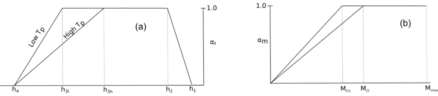
Figure 1. (a)Feddes et al. (1978) root water uptake reduction function.h2andh3are the threshold parameters for reduction in root water
uptake due to oxygen deficit and water deficit, respectively. The subscriptslandhstand for low and high potential transpirationTp.h1and
h4are the soil pressure head values above and below which root water uptake is zero due to oxygen and water deficit, respectively.(b)Root
water uptake reduction functionαmas a function of matric flux potentialM;MchandMclare the critical values ofMfor high and lowTp,
respectively, below which the uptake is reduced andMmaxis the maximum value ofM, dependent on soil type.
plants rehydrate to the same early morning water potentials on successive days (Taylor and Klepper, 1978).
In a macroscopic modelling approach, RWU is calculated as a sink termSin the Richards equation, which for the
ver-tical coordinate is given by
∂θ ∂t =
∂ ∂z
K(θ )∂h ∂z+1
−S, (2)
where θ (L3L−3) is the soil water content,h (L) the soil
water pressure head,K(L T−1) the soil hydraulic
conductiv-ity,t (T) the time, andz(L) the vertical coordinate (positive
upward). To apply Eq. (2), a functional expression for S is
needed. Physical equations in analogy to Ohm’s law have been suggested (see the review of Molz, 1981, for exam-ples) as well as expressions derived by upscaling microscopic models (De Willigen and van Noordwijk, 1987; Feddes and Raats, 2004; De Jong van Lier et al., 2008, 2013). Alter-natively, simple empirical models requiring less information about plant and soil hydraulic properties have also been pro-posed and are commonly used. Most of these models use the Feddes approach (Feddes et al., 1976, 1978), formulated as
S(z)=Sp(z)α(h[z]), (3)
whereα(h)is the RWU reduction function, defined by
Fed-des et al. (1978) as a piecewise linear function ofh(Fig. 1).
According to this approach, a reduction inSdue toα(h[z]) <
1 directly implies a transpiration reduction, causingα(h)to
be called a transpiration reduction function. Sp is the po-tential RWU, which is determined by partitioning popo-tential transpirationTpover depth. Several ways to estimateSpas a function of depth have been proposed (Prasad, 1988; Li et al., 2001, 2006; Raats, 1974), the most common being to dis-tributeTpover depth according to the normalized root length densityβ (L−1) defined as a fraction of root length density R(L L−3):
Sp(z)=Z R(z)
zm R(z)dz
Tp=β(z)Tp. (4)
Different expressions forαhave been suggested, normally
considering α a function of θ (e.g. Lai and Katul, 2000;
Jarvis, 1989), ofh (e.g. Feddes et al., 1978), or of a
com-bination of both (Li et al., 2006). Compared toθ,h seems
to be more feasible because of its relation to soil water en-ergy and the fact that obtained parameters of such a function would be more likely applicable to different soils. Some re-duction functions, generally associated with reservoir models for soil water balance, correlate RWU with the effective sat-uration. Regarding the shape of the reduction curve, smooth non-linear functions constrained between wilting point and saturation have been used, as well as piecewise linear func-tions, but they are all described by at least two empirical pa-rameters. The parameters of the smooth non-linear functions allow easy curve fitting, whereas in the piecewise functions they stand for the threshold at which RWU (or crop transpi-ration) is reduced due to drought stress, which has been an important parameter in crop water management.
Metselaar and De Jong van Lier (2007) showed for a verti-cally homogeneous root system that the shape ofαis not
early related to soil water content or to pressure head. A lin-ear relation betweenαand matric flux potential, a composite
soil hydraulic function defined in Eq. (5), is physically more plausible and was experimentally corroborated by Casaroli et al. (2010). Matric flux potential is defined as
M=
h
Z
hw
K(h)dh, (5)
wherehw is the soil pressure head at the wilting point.
Ac-cordingly, a more suitable expression forαwould be a
piece-wise linear function of M (Fig. 1). RWU can then be
2.1 Physically based root water uptake model
By upscaling earlier findings about water flow towards a single root in the microscopic scale, disregarding plant hy-draulic resistance (De Jong Van Lier et al., 2006; Metselaar and De Jong van Lier, 2007), De Jong van Lier et al. (2008) derived the following expression forS:
S(z)=ρ(z)[Ms(z)−M0(z)], (6)
whereMsis the bulk soil matric flux potential,M0the value
ofMat the root surface, andρ(z)(L−2) a composite
param-eter, depending onRand root radiusr0:
ρ(z)= 4
r02−a2rm2(z)+2[rm2(z)+r02]ln[arm(z)/r0]
, (7)
where rm(=√1/π R) (L) is the rhizosphere radius – de-fined as the half distance between neighbouring roots – and
a the distance relative torm–r0 where water content equals the average soil water content. In De Jong van Lier et al. (2013), this model is extended by taking into account the hy-draulic resistances to water flow within the plant. Dividing water transport within the plant into two physical domains (from root surface to root xylem to leaf), assuming no water changes within the plant tissue and by coupling Eq. (6) for water flow within the rhizosphere, they derived the following expression relating water potentials andTa:
h0(z)=hl+ϕ(Ms(z)−M0(z))+Ta
Ll, (8)
whereh0andhl(L) are the pressure heads at the root surface
and leaf, respectively,Ll(T−1) is the overall conductance of the root xylem-to-leaf pathway, andϕ(T L−1) is defined as
ϕ(z)=ρr
2 m(z)ln
r0 rx
2Kroot , (9)
where Kroot (L T−1) is the radial root tissue conductivity (referring to the pathway from the root surface to the root xylem), andrx(L) is the xylem radius. An analytical solution of Eq. (8) forh0orM0depends on an expression forM0(h0).
For a particular case of Brooks and Corey (1964) soils, a so-lution is provided by De Jong van Lier et al. (2013). For van Genuchten–Mualem-type soils, Eq. (8) can be solved numer-ically or by using a semi-analytical solution of Eq. (5) (De Jong van Lier et al., 2009). In any case, application of Eq. (8) requires a mathematical function relatingTaandhl. De Jong
van Lier et al. (2013) definedTaby a piecewise function
im-posing a limiting valuehwlonhl:
Tr=
1 :hl> hwl,
0≤Tr≤1 :hl=hwl,
0 :hl< hwl,
(10)
where Tr(=Ta/Tp) is the relative crop transpiration.
Be-cause Ta and hl are unknowns and Ta is undefined when
20 40 60 80 100 120 140
|hs|,m
10-9
10-8
10-7
10-6
10-5
10-4
10-3
10-2
10-1
Ro
ot
wa
ter
up
tak
e,
d
−
1
R=1 cm cm−3
R=0.1 cm cm−3
R=0.01 cm cm−3
-30 m
-50 m -70 m
-90 m -110 m
-130 m -150 m
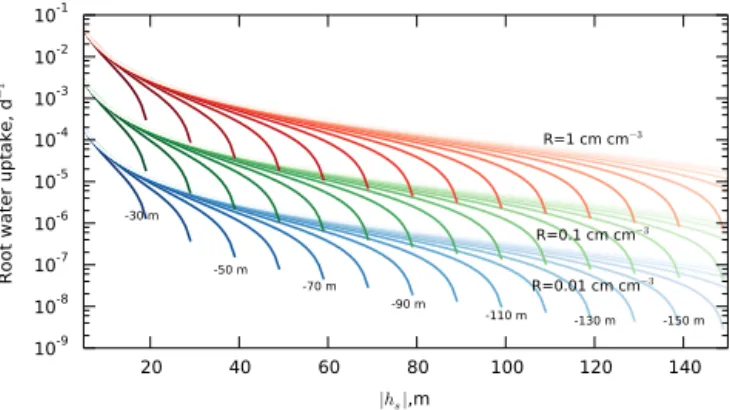
Figure 2.Root water uptake (RWU) as a function of soil
pres-sure headhsfor three values of root length density (0.01, 0.1, and
1.0 cm cm−3) and leaf pressure head values ranging from−30 to
−200 m by a−10 m interval shown by a colour gradient (lighter
colours indicate lower values; some values are indicated in the plot). Results were obtained by the analytical solution of Eq. (8) given by De Jong van Lier et al. (2013) for a special case of Brooks and
Corey (1964) soil. Plant transpiration was set to 1 mm d−1and the
soil and plant hydraulic parameters were taken from De Jong van Lier et al. (2013).
hl=hwl, the equation system cannot be solved analytically. An iterative solution was provided in De Jong van Lier et al. (2013) by defining a maximum transpiration rateTp,max, cor-responding toTa(Eq. 8) forhl=hwl. The system of
equa-tions is then solved by defining plant stress in terms of
Tp,max, according to the following boundary conditions:
unstressed conditions:Tp,max≥Tp :Ta=Tp, hl≥hwl,
stressed conditions: Tp,max< Tp :hl=hwl, Ta< Tp.
In the De Jong van Lier et al. (2013) model, crop water stress, a condition for whichTa< Tp, is defined at the crop
level (Tardieu, 1996) and begins whenhl=hw.Scan be
cal-culated using Eq. (6) by solving Eq. (8), with h0 (so M0) variable over the root zone and controlled by plant hydraulic properties and soil hydraulic conditions.
Figure 2 shows RWU for several values ofhl and helps to understand how RWU is distributed over depth.hlcan be regarded as a measure of water deficit stress over the whole root zone at crop level: as soil water is depleted,hlis reduced, thus increasing the driving force for RWU. As soil pressure headhsdecreases, high uptakes are only achieved by lower
hl. For a givenhlvalue, RWU is substantially reduced ashs
decreases. Ifhlis not reduced whilehsdecreases,Sbecomes
negative (although not shown in Fig. 2, negativeSis part of
the extension of each curve) and water will flow from root to soil, a phenomenon called hydraulic lift or hydraulic re-distribution (Jarvis, 2011). This situation occurs when parts of the root zone are wetter and RWU from these parts satis-fies transpiration demand, hencehlis not reduced.
content. Under homogeneous soil water distribution, RWU is partitioned proportionally toR. For heterogeneous
condi-tions, RWU for lowerRand higherR may be the same,
de-pending on the stress level (indicated byhl) and thehs (see
Fig. 2). This is in agreement with experimental results re-ported by several authors (Arya et al., 1975a, b; Green and Clothier, 1995; Verma et al., 2014), who found less densely rooted but wetter parts of the root zone to correspond to a significant portion of RWU when more densely rooted parts of the soil were drier, allowing the crop to maintain tran-spiration at potential rates. Empirical model concepts that only useRfor predicting RWU distribution over depth
(un-der non-stressed conditions) are most common, and there-fore these results have been interpreted as being due to a mechanism labelled “compensation” by which uptake is “in-creased” from wetter layers to compensate for the “reduc-tion” in the drier layers (Jarvis, 1989; Šim˚unek and Hop-mans, 2009). It is clear, however, that this compensation con-cept is found merely on a reference RWU distribution based onR, and it only needs to be explicitly addressed in empirical
models. In physical models, distinguishing compensation is not necessary since in such models “compensation” follows implicitly from the RWU mechanism.
In order to account for RWU pattern changes due to het-erogeneous soil water distribution (the so-called “compensa-tion”), several empirical models have been developed over the years. These models follow the general framework of the Feddes et al. (1978) model given by Eq. (3). Below we re-view these models and present a new empirical alternative. 2.2 Empirical root water uptake models accounting for
compensation
2.2.1 The Jarvis (1989) model
Jarvis (1989) defined a weighted-stress indexω(0≤ω≤1)
as
ω=
Z
zm
α(z)β(z)dz, (11)
where, differently from Feddes et al. (1978),αwas defined as
a function of the effective saturation. Whereas Feddes et al. (1978) assume the RWU reduction directly to be reflected in crop transpiration reduction, the Jarvis (1989) approach employs a so-called “whole-plant stress function” given by
Ta Tp =min
1, ω ωc
, (12)
whereωc is a threshold value ofωfor the transpiration re-duction. Substituting Eqs. (3) and (4) into Eq. (1) (the mass conservation principle) and combining with Eq. (12) results in
S(z)=Spα(z)α2, whereα2= 1 max{ω, ωc}
, (13)
whereα2is called the compensation factor of RWU, distinct
from Feddes’α(Eq. 3), and which can be derived by
defin-ingTaby Eq. (12). In the Jarvis (1989) model,αaccounts for
local reduction of RWU and transpiration reduction is com-puted by Eq. (12). Whenω=1, there is no RWU reduction
(α=1 throughout the root zone) and the model prediction
is equal to the Feddes model. Forωc< ω <1, uptake is re-duced in some parts of the root zone (as computed byα <1),
but the plant can still achieve potential transpiration rates by increasing RWU over the whole root zone by the factorα2. Whenω < ωc, even though the uptake is increased by the factorα2, the potential transpiration rate cannot be met. The threshold valueωcplaces a limit on the plant’s ability to deal with soil water stress. Whenωctends to 0, relative transpira-tion calculated by Eq. (12) tends to 1, and the plant can fully compensate for uptake and transpire at the potential rate if
α >0 at some position within the root zone.
In principle, any definition ofαis applicable in Eq. 11, and
commonly the Feddes et al. (1978) reduction function is used instead of the original Jarvis (1989) reduction function, e.g. in the HYDRUS model (Simunek et al., 2009). This modi-fied version of the Jarvis (1989) model, hereafter referred to as JMf, will be further analysed. Nevertheless, one should be careful in setting up and interpreting the threshold parameters of JMf. The Feddes et al. (1978) model does not account for compensation, and the threshold pressure head value below which RWU is reduced (h3) also represents the value below which transpiration is reduced, makingh3 values from the literature refer to this interpretation. Instead, in the JMf, the transpiration reduction only takes place whenω < ωc, and the soil pressure head in some layers is already supposed to be more negative thanh3. Therefore,h3in JMf is less
nega-tive than its namesake in the Feddes model. In that sense,h3
for the JMf is hard to determine experimentally. An option to do so would be by inverse modelling, optimizing outcomes of soil water flow models with experimental data.
Comparison to the De Jong van Lier et al. (2008) model The physical basis of Jarvis (1989), defined by Eqs. (11) to (13) with using anyα, has been questioned (Skaggs et al.,
2006; Javaux et al., 2013). However, the Jarvis model has, to some extent, a physical basis, and a comparison with the physically based model of De Jong van Lier et al. (2008) can be made, as demonstrated in Jarvis (2010, 2011). This is dis-cussed in the following.
De Jong Van Lier et al. (2006) derived Eq. (6) to describe RWU. Crop transpiration is obtained by integrating Eq. (6) overzmas defined in Eq. (1), leaving two unknowns:M0and
Ta. To solve for these, De Jong van Lier et al. (2008) defined
Taas a piecewise function:
Ta
Tp=min
1,Tp,max Tp
whereTp,max(L T−1), differently from the definition in the De Jong van Lier et al. (2013) model, is the maximum tran-spiration rate reached when the root surface pressure head is constant over depth and equal to a limiting valuehw. For
such a conditionM0=0 andTp,maxis given by
Tp,max=
Z
zm
ρ(z)M(z)dz. (15)
From Eq. (14) we see that drought stress occurs when
Tp,max< Tp. At the onset of drought stress,Ta=Tp,max. Un-der this condition,M0=0 andS(z)becomes
S(z)=ρ(z)M(z). (16)
When Tp,max> Tp, Ta=Tp (no drought stress), and M0 (>0) is given by
M0= Z
zm
ρ(z)M(z)dz−Tp
R
zmρ(z)dz
. (17)
Jarvis (2011) observed the similarities between Eqs. (14) and (12) of the models, as well as the algebraic similar-ity between ω (Eq. 11) and Tp,max (Eq. 15). Thus, Jarvis (2010) showed that both models provide the same results un-der drought stress ifαandβ(z)are defined as follows:
α= M
Mmax, (18)
β=Z ρ(z)
zm ρ(z)dz
, (19)
whereMmaxis the maximum value ofM(i.e. ath=0). By
substituting Eq. (18) and (19) into Eq. (15) and comparing Eq. (12) with Eq. (14),ωcis found to be equal to
ωc=
Tp
Mmax Z
zm ρ(z)dz
. (20)
Substitution of Eqs. (18) to (20) into Eqs. (12) and (11) re-sults in Eq. (16) of the De Jong van Lier et al. (2008) model for stressed conditions. Consequently, both models provide the same numerical results. For unstressed conditions, anal-ogous substitution results in
S(z)=ρ(z)M(z) Tp Tpmax =
ρ(z)M(z) R
zm ρ(z)M(z)dz
Tp. (21)
Equation (21) is different from Eq. (6) and, therefore, the models cannot be correlated for these conditions. The Jarvis (1989) model predicts RWU by a weighting factor between
ρ and M throughout rooting depth. Defining α and β by
Eqs. (18) and (19), respectively, allowed us to correlate both models only for stressed conditions. These definitions and the resulting model will be further analysed.
2.2.2 The Li et al. (2001) model
Li et al. (2001) proposed to distribute potential transpiration over the root zone by a weighted stress indexζ, being a
func-tion of both root distribufunc-tion and soil water availability:
ζ (z)= α(z)R(z)
lm
R
zmα(z)R(z)
lmdz, (22)
whereα(–) andR(L L−3) were previously defined and the
exponentlm is an empirical factor modifying the shape of RWU distribution over depth. Originally, thelmvalues were based on experimental works. For 0< lm<1, the RWU in sparsely rooted soil layers is increased in the attempt to mimic compensation. Forlm>1, which has no maximum, the uptake from more densely rooted soil layers increases. Thus,Spis given by
Sp=ζ (z)Tp (23)
and RWU is calculated by substituting Eq. (23) into Eq. (3), following the Feddes approach.
As an alternative to the Jarvis (1989) model,Spcan be de-fined as function of root length density and soil water avail-ability distribution. Compensation is directly accounted for by the weighted stress index in Eq. (22). However, usingαto
represent soil water availability in Eq. (22) does not mimic properly the compensation mechanism. Compensation may take place before transpiration reduction. Usingαin Eq. (22)
means that compensation will only take place after the on-set of transpiration reduction whenαin one or more layers
is smaller than 1. Thelmparameter may also be interpreted as to account for compensation under non-stressed condition. However, compensation as well as the shape of the RWU dis-tribution are likely to change when a soil becomes drier, and a constantlmcannot account for that.
2.2.3 The Molz and Remson (1970) and Selim and Iskandar (1978) models
Decades before Li et al. (2001), Molz and Remson (1970) and Selim and Iskandar (1978) already suggested to dis-tribute potential transpiration over depth according to root length density and soil water availability. Instead of usingα
to account for soil water availability, they used soil hydraulic functions. The weighted stress index was defined as
ζ (z)=Z Ŵ(z)R(z)
zm
Ŵ(z)R(z)dz
, (24)
whereŴ is a soil hydraulic function to account for water
availability. Molz and Remson (1970) used soil water diffu-sivityD(L2T−1), and Selim and Iskandar (1978) used soil
is then calculated by substituting Eq. (24) into Eq. (23) and then into Eq. (3) following the Feddes approach.
These models may better represent RWU and compensa-tion than the Li et al. (2001) model. The compensacompensa-tion is implicitly accounted for by means of Ŵ inζ. Since Ŵ
de-creases as soil water is depleted, in a heterogeneous soil wa-ter distributionζ in wetter layers is relatively increased
be-cause the overallR
ŴRdzis reduced due to the reduction of Ŵin drier, more densely rooted soil layers. Differently from
the Li et al. (2001) model, this change in RWU distribution can occur before the onset of transpiration reduction. Heinen (2014) compared different types of Ŵ in Eq. (24) such as
the relative hydraulic conductivity (Kr=K/Ksat) and rela-tive matric flux potential (Mr=M/Mmax), among others. He found large differences in predicted RWU patterns for differ-ent forms ofŴ, but did not indicate a preference for a specific
one.
2.2.4 Proposed empirical model
In describing soil water availability, the matric flux potential
M may be a better choice than K or D, since it integrates K andhorDandθ (Raats, 1974; De Jong van Lier et al.,
2013). We propose a new weighted stress index, defined as
ζm(z)=
RlmM(h)
Z
zm
RlmM(h)dz
. (25)
The exponentlm provides additional flexibility on distribut-ing TP over depth, as also shown by Li et al. (2001). The proposed model differs from Li et al. (2006) only on the hy-draulic property to account for soil water availability. Theα
function used in Li et al. (2006) can only alter RWU dis-tribution after the onset of transpiration reduction, as com-mented earlier. Contrastingly, M affects RWU distribution
before transpiration reduction, integrating the effect of both
Kandh.
The RWU can then be obtained by inserting Eq. (25) into Eq. (23) (Sp) and multiplying by any reduction function, such
as the Feddes et al. (1978) and proposed reduction func-tions. In other words, the model follows the Feddes approach, which computes RWU by the two mentioned steps, which differ only with respect to the waySp is obtained: Eq. (25) (multiplied byTp) versus Eq. (4).
3 Material and methods 3.1 Applied models
Table 1 summarizes the empirical RWU models evaluated in this study. They all follow the original Feddes model (Eq. 3), but differ in how RWU is partitioned over rooting depth or howαis defined. For each model, except for Jarvis
(2010), we defined a modified version by substituting the
Feddes reduction function by the proposed reduction func-tion (Fig. 1b), and these modified versions were also evalu-ated. The threshold values of the Feddes et al. (1978) reduc-tion funcreduc-tion for anoxic condireduc-tions (h1andh2) were set to
zero. The value of the parameterh4was set to−150 m. The
other parameters of the models were obtained by optimiza-tion as described in Sect. 3.2.
All these models were embedded as sub-models in the SWAP ecohydrological model (Van Dam et al., 2008), allow-ing us to solve Eq. (2) and to apply it to different scenarios of root length density, atmospheric demand, and soil type (de-scribed in Sect. 3.2) to analyse the behaviour and sensitivity of the models. Simulation results of SWAP in combination with each of the RWU models were compared to the SWAP predictions in combination with the physical RWU model de-veloped by De Jong van Lier et al. (2013).
The values of the De Jong van Lier et al. (2013) model parameters used in the simulations are listed in Table 2. The values ofKroot andLl are within the range reported by De
Jong van Lier et al. (2013). 3.2 Simulation scenarios 3.2.1 Drying-out simulation
Boundary conditions for drying-out simulations were no rain/irrigation and a constant atmospheric demand (poten-tial transpiration) over time. The simulation continued until simulated crop transpiration by the physical RWU model ap-proached zero. Soil evaporation was set to zero, making soil water depleted only due to RWU or bottom drainage. The free drainage (unit hydraulic gradient) at the maximum root-ing depth was the bottom boundary condition. The soil was initially at hydrostatic equilibrium with a water table located at 1 m depth. We performed simulations for two levels of at-mospheric demand given by potential transpiration (Tp) of 1 and 5 mm d−1. We also considered three soil types and three levels of root length density, as described in the following. Soil type
Soil data for three top soils from the Dutch Staring series (Wösten et al., 1999) were used. The physical properties of these soils are described by the Mualem-van Genuchten functions (Mualem, 1976); (Van Genuchten, 1980) for the
K−θ−hrelations:
2 = [1+ |αh|n](1/n)−1 (26)
K = Ksat2λ[1−(1−2n/(n−1))1−(1/n)]2 (27)
where2=(θ−θr)/(θs−θs);θ,θrandθsare water content,
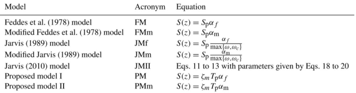
Table 1.Summary of empirical models used in this study.αf andαmare the Feddes et al. (1978) (Fig. 1a) and proposed reduction functions
(Fig. 1b),Sp(Eq. 4) is the potential root water uptake,ω(Eq. 11) andωcare the weighted stress index and threshold value in the Jarvis
(1989) model, andζm(Eq. 25) is the weighted stress index in the proposed models.
Model Acronym Equation
Feddes et al. (1978) model FM S(z)=Spαf
Modified Feddes et al. (1978) model FMm S(z)=Spαm
Jarvis (1989) model JMf S(z)=Spmaxα{ω,ωf c}
Modified Jarvis (1989) model JMm S(z)=Spmaxα{ω,ωm c}
Jarvis (2010) model JMII Eqs. 11 to 13 with parameters given by Eqs. 18 to 20
Proposed model I PM S(z)=ζmTpαf
Proposed model II PMm S(z)=ζmTpαm
Table 2.Values of the parameters of the De Jong van Lier et al.
(2013) model used in the simulations.hwsis the limiting valuehw
in Eq. (5) for the empirical models.
Parameter Value Unit
r0 0.5 mm rx 0.2 mm
Kroot 3.5·10−8 m d−1
Ll 1·10−6 d−1
hws −150 m
hwl −200 m
in Table 3. These soils are identified in this text as clay, loam and sand.
Root length density distribution
Three levels of root length density were used, according to the range of values normally found in the literature. We con-sidered low, medium and high root length density for average crop values equal to 0.01, 0.1 and 1.0 cm cm−3, respectively. For all cases, we set the maximum rooting depthzmaxequal to 0.5 m. Root length density over depthzwas described by
the exponential function:
R(zr)=R0(1−zr)exp−bzr, (28)
whereR0(L L−3) is the root length density at the soil sur-face,b (–) is a shape-factor parameter, andzr (=z/zmax) is the relative soil root depth. The term(1−zr)in Eq. (28) guar-antees that root length density is zero at the maximum rooting depth. The parameterR0is hardly ever determined, whereas
the average root length density of crops Ravg is usually
re-ported in the literature. AssumingRof such a crop given by
Eq. (28), it can be shown that 1
Z
0
R0(1−zr)exp−bzrdzr=Ravg. (29)
0.0 0.5 1.0 1.5 2.0 2.5 3.0 3.5 4.0 4.5
Root length density cm cm
−3
0.0
0.2
0.4
0.6
0.8
1.0
Relative depth
b=0.1
b=1.0
b=2.0
b=3.0
Medium
RavgLow
RavgFigure 3.Root length density distribution over depth calculated by
Eq. (30) for several values ofband Ravg=1.0 cm cm−3and for
low and mediumRavgwithb=2.
Solving Eq. (29) forR0and substituting into Eq. (28) gives
R(zr)=
b2Ravg
b+exp−b−1(1−zr)exp−
bzr (b >0). (30)
Figure 3 showsR(zr)calculated from Eq. (30) for differ-ent values ofbandRavg=1 cm cm−3. Asbapproaches zero,
Eq. (30) tends to become linear; however, it is not defined for
b=0. In our simulationsbwas arbitrarily set equal to 2.0.
Optimization
Table 3.Mualem–van Genuchten parameters for three soils of the Dutch Staring series (Wösten et al., 1999) used in simulations.θsandθr
are the saturated and residual water content, respectively;Ksis saturated hydraulic conductivity andα,λ, andnare fitting parameters.
Staring soil ID Textural Reference in θr θr Ks α λ n
class this paper m m−3 m m−3 m d−1 m−1 – –
B3 Loamy sand Sand 0.02 0.46 0.1542 1.44 −0.215 1.534
B11 Heavy clay Clay 0.01 0.59 0.0453 1.95 −5.901 1.109
B13 Sand loam Loam 0.01 0.42 0.1298 0.84 −1.497 1.441
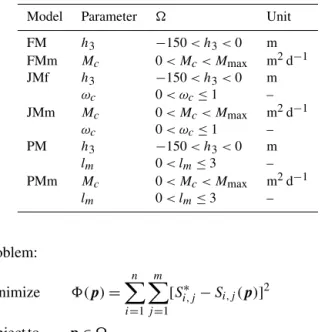
Table 4.Parameters of the root water uptake models estimated by
optimization and their respective constraints.
Model Parameter Unit
FM h3 −150< h3<0 m
FMm Mc 0< Mc< Mmax m2d−1
JMf h3 −150< h3<0 m
ωc 0< ωc≤1 –
JMm Mc 0< Mc< Mmax m2d−1
ωc 0< ωc≤1 –
PM h3 −150< h3<0 m
lm 0< lm≤3 –
PMm Mc 0< Mc< Mmax m2d−1
lm 0< lm≤3 –
problem:
minimize 8(p)= n
X
i=1 m
X
j=1
[Si,j∗ −Si,j(p)]2
subject to p∈ (31)
where8(p)is the objective function to be minimized,Si,j∗
is the RWU simulated by the SWAP model together with the De Jong van Lier et al. (2013) model at time i(time
inter-val of 1 day) and depthj (of each soil layer), andSi,j(p)is the corresponding RWU predicted by SWAP in combination with one of the empirical models shown in Table 1.pis the
model parameter vector to be optimized, constrained in the domain. Bothpandvary depending on the empirical
RWU model used. Table 4 shows the parameters of each em-pirical RWU model that were optimized and their respective constraints.mis the number of soil layers (50 soil layers
of 1 cm thickness) andnis the duration, in days, of the
simu-lation. The Jarvis (2010) model has no empirical parameters and therefore requires no optimization.
Equation (31) was solved using the PEST (Parameter ES-Timation) tool (Doherty et al., 2005) coupled to the adapted version of SWAP. PEST is a non-linear parameter estima-tion program that solves Eq. (31) by the Gauss–Levenberg– Marquardt (GLM) algorithm, searching for the deviation, ini-tially along the steepest gradient of the objective function and switching the search gradually to the Gauss–Newton algorithm as the minimum of the objective function is ap-proached. Upon setting PEST parameters, we made reference
runs of SWAP with each empirical model using random val-ues ofpaiming to assess the ability of PEST to retrievep.
These reference runs allowed us to properly set up PEST for our case. For highly non-linear problems as in Eq. (31), the optimized parameter set depends on the initial values ofb. We used five random sets of initial values forpin order to guarantee that GLM encountered the global minimum and also to check the uniqueness of the solution. Runs led to the same minimum in most cases, but if not, the minimum was compared and a fit run was made again.
The optimizations were performed for the drying-out sim-ulation only. This guaranteed that RWU predictions from SWAP corresponded to the best fit of each empirical model to the De Jong van Lier et al. (2013) model. This analysis aimed to investigate the capacity of the empirical RWU models to mimic the RWU pattern predicted by the De Jong van Lier et al. (2013) model. The optimized parameters were subse-quently used to evaluate the models in an independent grow-ing season scenario.
3.2.2 Growing season simulations
In the growing season simulation, all models were evaluated by simulating the transpiration of grass with weather data from the De Bilt weather station, the Netherlands (52◦06′N; 5◦11′E), for the year 2006. The same root system distribu-tion as in the drying-out simuladistribu-tions was used, i.e. a crop with roots exponentially distributed over depth as Eq. (30) (b=2.0) down to 50 cm below the soil surface. We also
per-formed simulations for the same three types of soils and root length densities. In all cases the crop fully covered the soil with a leaf area index of 3.0. Daily reference evapotranspira-tion ET0was calculated by SWAP using the FAO Penman– Monteith method (Allen et al., 1998). In the SWAP model, a potential crop evapotranspiration ETpis obtained by mul-tiplying ET0 by a crop factor, which for the grass vegeta-tion was set to 1 (Van Dam et al., 2008). ETp was parti-tioned over potential evaporationEpandTp using
parame-ter values for common crops given in the SWAP model (see Van Dam et al., 2008, for details).
inter-1
Tr
Low R
0 38 76 114 152 0
10 20 30 40
Depth, cm
Tp
=
1 m
m
d
−
1
Medium R
0 38 76 114 152
High R
0 -100
hl
, m
0 38 76 114 152 0
0.001 0.002 0.003 0.004 0.006 0.007
RWU
1
Tr
0 9 18 27 36 Time, d 0
10 20 30 40
Depth, cm
Tp
=
5 m
m
d
−
1
0 9 18 27 36 Time, d
0 -100
hl
, m
0 9 18 27 36 Time, d
0 0.005 0.01 0.02 0.02 0.03 0.03
RWU
(a)
(b)
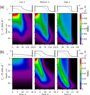
Figure 4.Time–depth root water uptake (RWU, d−1) pattern, leaf
pressure head (hl, dashed line), and relative transpiration (Tr,
con-tinuous line) simulated by the SWAP model together with the De Jong van Lier et al. (2013) model for clay soil, two levels of
poten-tial transpirationTp: 1 and 5 mm d−1(first and second lines of the
plots, respectively), and three levels of root length densityR: low,
medium, and high (indicated at the top of the figure).
polated for intermediate levels of Tp. For Tp higher than 5 mm d−1andTplower than 1 mm d−1, the values estimated for 5 and 1 mm d−1, respectively, were used.
As in the drying-out simulations, the bottom boundary condition was free drainage. Initial pressure heads were ob-tained by iteratively running SWAP starting with the final pressure heads of the previous simulation until convergence.
4 Results and discussion 4.1 Drying-out simulation
4.1.1 Root water uptake pattern: De Jong van Lier (2013) model
In this section we first focus on the behaviour of the De Jong van Lier et al. (2013) model in predicting RWU for the eval-uated scenarios in the drying-out experiment. Figure 4 shows the RWU patterns for the case of the clay soil for the three evaluated root length densitiesRand the two levels of
poten-tial transpirationTp. It can be seen howRandTpaffect RWU distribution and transpiration reduction as the soil dries out. The onset and shape of transpiration reduction is affected by the RWU pattern. For low R, the low number of roots
in deeper layers is not sufficient to supply high RWU rates. When the upper layers become drier, transpiration reduction follows immediately. Under medium and highR, the RWU
front moves gradually downward as water from the upper layers is depleted. Comparing from high to mediumR, the
RWU front goes even deeper, and transpiration is maintained at potential rates for a longer time (Fig. 4). Accordingly, the plant exploits the whole root zone and little water is left when transpiration reduction onsets, causing an abrupt drop in tran-spiration. RegardingTp, the RWU patterns are very similar for both evaluated rates, differing only in time scale: for high
Tpthe onset of transpiration reduction and the shift in RWU front occur earlier. The uptake patterns for the sand and loam soil (not shown here) are very similar. However, for the sand soil potential transpiration is maintained a little longer and more water is extracted from deeper layers. For the loam soil, the onset of transpiration reduction occurred earlier.
The leaf pressure headhlover time shown in Fig. 4
illus-trates how the model adaptshltoRandTplevels in a drying
soil. Initially all scenarios have the same water content dis-tribution and lowerhl values are required for lowR or high Tpscenarios to supply potential transpiration rates. As soil becomes drier,hl is decreased to increase the pressure head gradient between bulk soil and root surface, thus maintain-ing RWU correspondmaintain-ing to the demand. Therefore, uptake in wetter layers becomes more important. Transpiration reduc-tion only onsets whenhl reaches the limiting leaf pressure headhwl (= −200 m), after significant changes in the RWU patterns, characterized by increased uptake from deeper lay-ers.
For the highTp–lowR scenarios, transpiration reduction
starts on the first day of simulation, although the soil is relatively wet. This is a case of transpiration reduction un-der non-limiting soil hydraulic conditions due to high atmo-spheric demand (Cowan, 1965). For such conditions, the high water flow within the plant required to meet the atmospheric demand cannot be supported by the root system with a low
Rand hydraulic parameters given in Table 2. Higher
rais-Table 5.Optimal parameters of each empirical model for all scenarios in the drying-out experiment.
FM FMm JMf JMm PM PMm
Soil Tp R h3 Mc h3 ωc Mc ωc h3 lm Mc lm
mm d−1 cm cm−3 cm cm2d−1 cm – cm2d−1 – cm – cm2d−1 –
clay 1 0.01 −1968.7 0.213 −284.5 0.711 0.366 0.494 −1615.7 1.322 0.227 1.290
clay 1 0.10 −1211.0 0.329 −132.4 0.196 0.944 0.024 −7579.9 0.869 0.076 0.884
clay 1 1.00 −1.7 0.950 −0.0 1.000 5.971 0.004 −10673.7 0.354 0.022 0.342
loam 1 0.01 −7588.1 0.334 −5.0 0.457 22.483 0.016 −6927.6 1.086 0.408 1.084
loam 1 0.10 −6085.6 0.487 −93.9 0.126 25.721 0.002 −11795.6 0.911 0.113 0.917
loam 1 1.00 −17.0 5.014 −48.0 1.000 106.223 0.000 −10878.8 0.561 0.058 0.553
sand 1 0.01 −1014.0 0.146 −291.6 0.942 0.288 0.436 −621.2 1.262 0.149 1.252
sand 1 0.10 −1122.6 0.115 −113.6 0.407 1.925 0.005 −2351.3 1.179 0.024 1.159
sand 1 1.00 −3.9 0.338 −0.0 1.000 25.887 0.000 −3158.0 0.717 0.005 0.706
clay 5 0.10 −1397.7 0.334 −218.4 0.325 0.395 0.271 −5537.2 1.512 0.196 1.449
clay 5 1.00 −260.6 0.792 −135.3 0.148 1.212 0.013 −6745.0 0.672 0.088 0.687
loam 5 0.10 −5236.5 0.784 −0.0 0.277 2.306 0.100 −8322.9 1.165 0.488 1.157
loam 5 1.00 −1249.5 2.563 −292.9 0.161 28.143 0.001 −8630.0 0.833 0.224 0.838
sand 5 0.10 −918.0 0.190 −556.2 0.432 4.154 0.018 −1273.9 1.612 0.083 1.510
sand 5 1.00 −582.3 0.533 −342.5 0.193 4.888 0.001 −3582.3 1.272 0.012 1.240
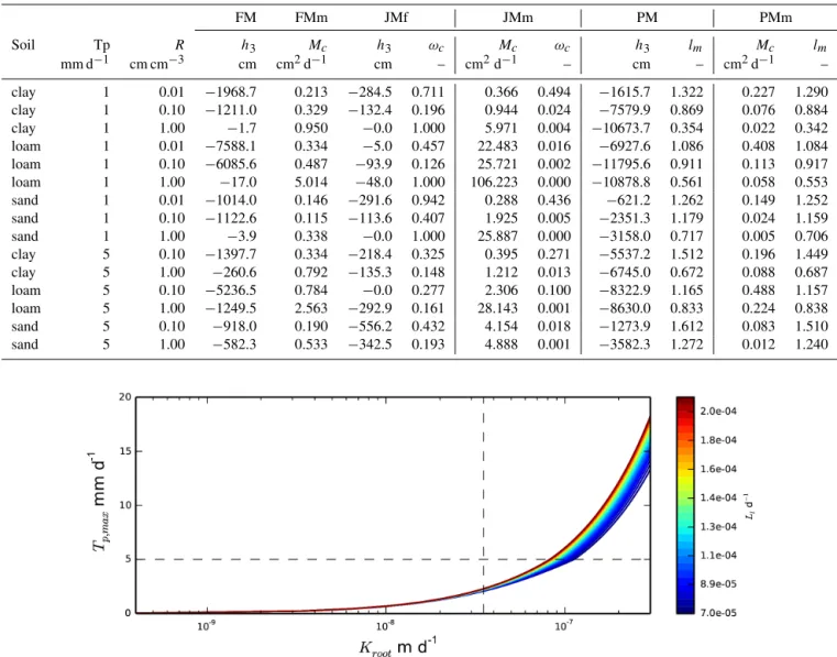
Figure 5.Maximum possible transpirationTp,maxas a function of root hydraulic conductivityKroot for some values of the overall
con-ductance over the root-to-leaf pathwayLl computed by the De Jong van Lier et al. (2013) model for a rooting depth of 0.5 m, low root
length density, and a constant soil pressure head over depth equal to−1 m for sandy soil. The dashed vertical line highlights the value of
Kroot=3.5·10−8m d−1that was used in our simulations. The horizontal dashed line highlights the value of potential transpiration.
ingKrootto about 10−7m d−1. This can also be achieved by
decreasinghwl(not shown in Fig. 5).
In the field, transpiration rate and root length density are related to each other: a high transpiration rate only oc-curs in a high leaf area, and a high leaf area implies a high root length density. Thus, even under very dry and hot weather conditions, a crop with a low R may not be
able to realize a high transpiration rate. Furthermore, crop transpiration depends on the stomatal conductance. In the De Jong van Lier et al. (2013) model, this is implicitly taken into account by the simple relationship between hl andTa. However, stomatal conductance is relatively complex and de-pends on several environmental factors such as air tempera-ture, solar radiation, and CO2concentration. Therefore, high
potential transpiration rates may not be achieved because of the stomatal conductance reduction due to temperature or so-lar radiation. This behaviour could be simulated by the cou-pling of the De Jong van Lier et al. (2013) model to stomatal conductance models, such as the Tuzet et al. (2003) model.
4.1.2 Root water uptake pattern predicted by the empirical models
predictions were obtained with respective optimized param-eters as shown in Table 5 and are discussed in Sect. 4.1.4, and therefore represent the best fit with VLM.
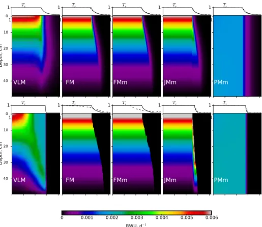
The RWU patterns simulated by VLM and the empirical models for the sandy soil and highRscenario are shown in
Figs. 6 and 7 for low and highTp, respectively. Both versions
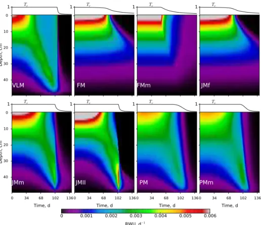
of the Feddes model (FM and FMm) predicted enhanced RWU from the upper soil layers. When the soil pressure head (hs for FM) or soil matric flux potential [Ms for FMm] is greater than the threshold value for uptake reduction, these uptake patterns are equivalent to the verticalR distribution.
For conditions drier than the threshold value (whenαf and αmare less than 1), the predicted RWU patterns by the mod-els become different (Figs. 6 and 7).
When reducing RWU for a period depending onR,Tp, and
h3, RWU from the upper soil layers predicted by FM rapidly
decreases to zero. This zero-uptake zone expands downward as soil dries out. On the other hand, the uptake predicted by FMm is substantially reduced right after the onset of transpi-ration reduction, proceeding at lower rates and for a much longer time until approaching zero. These features become evident by comparing the shapes of both reduction functions (Fig. 8). αm is linear withM after M > Mc, but it is con-cavely shaped as a function ofh– as also shown by
Metse-laar and De Jong van Lier (2007) and De Jong van Lier et al. (2009). This makesαmdecrease abruptly forM > Mc, caus-ing a substantial decrease in RWU even whenh is slightly
below the threshold value. Therefore, RWU proceeds at low rates for a longer time. In contrast and due to the linear shape of αf, RWU predicted by FM remains higher for a longer time afterh < h3. FM does not predict an abrupt change in
RWU patterns, especially whenTp is low (Fig. 6). Whenh
approachesh4,αf is still relatively high and RWU makesh decrease rapidly. Another diverging feature betweenαf and αm, also shown in Fig. 8, is that the shape ofαmvaries with
soil type (regardless of the value of its threshold parameter
Mc), whereas αf does not. These different features of the reduction functions also affect the matching values of the pa-rameters, as discussed below. Although the choice of the re-duction function affects transpiration over time only slightly, RWU patterns are strongly affected (Figs. 6 and 7).
The RWU patterns predicted by the JMf and JMm models can be very different, as shown by Fig. 6 for the highR–low Tpscenario. In this scenario, the JMf model did not predict any compensation because the optimal ωc equalled 1 (Ta-ble 5) – thus becoming identical to FM – and the optimalh3
values for JMf and FM were similar. In Fig. 6, althoughh3
values for FM and JMf (ωc=1) are close to zero, the plant transpiration is nearTpfor a prolonged time due to a small
reduction ofα. These highR–lowTpscenarios with a highR
in deep soil layers allow RWU at higher rates when surface soil layers become drier (as predicted by VLM). Then, the reduction ofωc, an attempt to numerically predict compen-sation with JMf, makes the RWU pattern deviate even more from the VLM pattern. This is illustrated in Fig. 6 and by the
optimalh3andωcvalues shown in Table 5. In order to mimic the VLM uptake patterns, the value ofh3for all soil types in
this scenario was equal or close to zero. Decreasingh3orωc to simulate compensation makes JMf predict higher uptake from upper layers, increasing the discrepancy between the models. The optimalωcfor all soil types was equal to 1 (in other words: there was no compensation). RWU in the up-per layers predicted by VLM is substantially reduced within a few days, whereas reducingωcin the JMf model to predict compensation has the side effect of causing an increase in uptake from upper layers. The model, therefore, is not able to adequately mimic the scenarios with compensation eval-uated here. On the other hand, the JMm model was able to reproduce considerably well the VLM pattern for the eval-uated scenarios due to the shape ofαm as discussed above. As soon asM < Mcin the upper layers, RWU decreased at a higher rate, compensated for by increasing uptake from the wetter, deeper layers. This agrees more closely with VLM predictions.
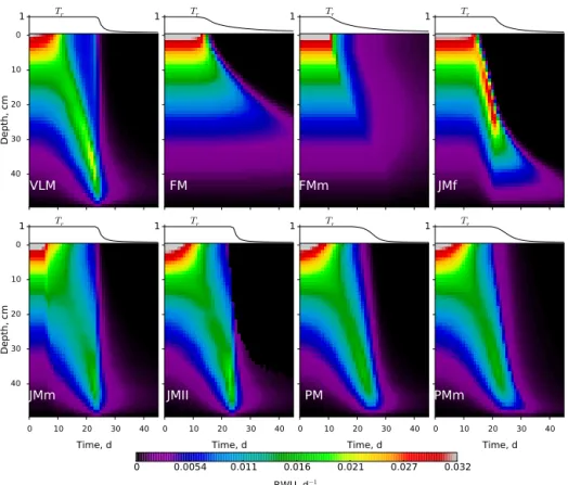
For highTp(Fig. 7), the JMf model can predict
compen-sation (ωc<1); however, its predicted RWU pattern is quite different from JMm and VLM. JMf predicts a higher longer-lasting RWU near the soil surface than the other models that account for compensation. This makes soil water depletion more intense and RWU from these layers to cease sooner when hs becomes lower thanh4. At this point, Ta is pre-dicted to continue to be equal toTpbecause of the low op-timalωc (=0.19), which increases RWU from the deeper layers wherehis close or equal toh4. JMm performed very differently, predicting uptake over the first few days (when
Ms> Mc) in accordance withRdistribution. AfterM < Mc in the upper soil layers, the RWU pattern started to change gradually and RWU increased at lower depths.
The proposed models (PM and PMm) are capable of pre-dicting RWU patterns similar to VLM. For the lowTp–high Rscenario (Fig. 6), RWU is more uniformly distributed over
depth than in the VLM model for the first days and uptake from upper layers is lower than that predicted by the VLM model. For highTp (Fig. 7), these models better represent RWU patterns and, in general, differences in predictions of RWU between the proposed models are small. The shape of the transpiration reduction over time, however, is smoother than predicted by the VLM model. Concerning the relative transpiration curve, the proposed models appear to be less precise than the other models that account for RWU com-pensation.
JMII does not mimic well the RWU pattern predicted by VLM for the highR–lowTpscenarios. It overestimates
up-take from surface layers during the first days. Before the onset of transpiration reduction, uptake from upper layers reaches zero, but it is compensated for by a higher uptake from deeper layers. The model is very sensitive to bothR
1 Tr
0
10
20
30
40
Depth, cm
VLM
0 0.001 0.002 0.003 0.004 0.005 0.006 RWU, d−1
1 Tr
FM
1 Tr
FMm
1 Tr
JMf
1 Tr0 34 68 102 136
Time, d 0
10
20
30
40
Depth, cm
JMm
1 Tr
0 34 68 102 136
Time, d
JMII
1 Tr
0 34 68 102 136
Time, d
PM
1 Tr
0 34 68 102 136
Time, d
PMm
Figure 6.Time–depth root water uptake (RWU) pattern and relative transpiration (Tr) simulated by the SWAP model in combination with the
De Jong van Lier et al. (2013) reduction function and the empirical models, for the sand soil at high root length density andTp=1 mm d−1.
does not perform well in the other scenarios with low and mediumR(data not shown here).
Comparing RWU predictions from JMf and JMII, the Jarvis-type models are affected by the definition of α. This
becomes clear from Fig. 9, which shows the α of JMII
(Eq. 18) as a function of hs andωc (Eq. 20) for different soil types, expressed by Mmax. Theα function shows that
even though the soil resistance increases as the soil becomes drier, definingαby Eq. (18) does not seem plausible. In this
case,αis suddenly reduced when the soil is still near
satura-tion. Whenhs=1 m, for instance,αis much lower than 0.5.
Such behaviour is not reasonably compatible with for theα
concept. The ωc values are also extremely low. The lowα values are, however, balanced by highα2values (due to low
ω and ωc values), leading to suitable values of RWU in a given soil layer. Nevertheless, the magnitudes of αandωc are conceptually questionable. Therefore, we conclude that (i) the ωc value in Jarvis-type models, which sets the com-pensation level, depends on the definition ofα. For instance,
for the original Jarvis (1989) model, ωc=0.5 corresponds to a moderate level of compensation. Surely, this would not hold ifαwere defined by Eq. (18); (ii) comparing the Jarvis
(1989) to the De Jong van Lier et al. (2008) model led to a rather unrealisticαfunction, and its behaviour does not
prop-erly represent theαconcept. This may be caused by the fact
that the De Jong van Lier et al. (2008) model does not take
into consideration the plant hydraulic resistances. This might explain the rapid decline ofαnear saturation. The
threshold-type functions seem to be more feasible.
The fact that JMII is more sensitive to bothRandM, as
stated above, when compared to the otherM-based models is
attributed to theαfunction and the derived equations to
ex-press their parameters (Eqs. 19 and 20). It can be seen from Fig. 9c thatβ defined by Eq. (19) (β of JMII) tends to be
higher whenRincreases and lower whenRdecreases
com-pared to theβ of JMf and JMm. Thereby, for the first days
of simulations when the soil hydraulic conditions tend to be rather uniform over depth, JMII overestimates RWU com-pared to VLM predictions. This becomes more important for the highR–lowTpscenarios. For such conditions, the RWU over depth predicted by the VLM tends to be more uniform, which seems reasonable as the low transpiration demand can be met by any smallRin deeper soil depths. After some time,
the discrepancies between VLM and JMII tend to increase, since the higher RWU in the upper layers reducesh; thus,
because of theαshape of JMII, RWU in the upper layers is
1 Tr
0
10
20
30
40
Depth, cm
VLM
0 0.0054 0.011 0.016 0.021 0.027 0.032 RWU, d−1
1 Tr
FM
1 Tr
FMm
1 Tr
JMf
1 Tr
0 10 20 30 40
Time, d 0
10
20
30
40
Depth, cm
JMm
1 Tr
0 10 20 30 40
Time, d
JMII
1 Tr
0 10 20 30 40
Time, d
PM
1 Tr
0 10 20 30 40
Time, d
PMm
Figure 7.Time–depth root water uptake (RWU) pattern and relative transpiration (Tr) simulated by the SWAP model in combination with the
De Jong van Lier et al. (2013) reduction function and the empirical models, for the sand soil at high root length density andTp=5 mm d−1.
0 20 40 60 80 100 120 140 160
|
h
|,m
0.0 0.2 0.4 0.6 0.8 1.0
α
m,
α
fT
p =1mm d
−1Clay Loam
Sand
0 20 40 60 80 100 120 140 160
|
h
|,m
0.0 0.2 0.4 0.6 0.8 1.0
T
p =5mm d
−1Clay Loam
Sand
(a) (b)
Figure 8. Feddes et al. (1978) (αf, grey lines) and proposed (αm, black lines) water uptake reduction functions as a function of soil
pressure headhusing their respective optimized parameters for the scenario of high root length density, three types of soil, and two potential
transpiration levels.
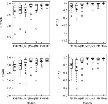
4.1.3 Statistical indices
The performance of the empirical models was analysed by the coefficient of determinationr2and the model efficiency
coefficientE(Nash and Sutcliffe, 1970) calculated by
com-paring to the RWU and relative transpiration predicted by VLM. For the low R–highTpscenarios, the VLM predicts water stress (Ta< Tp) from the beginning of the simulation as discussed in Sect. 4.1.1. The empirical models (except for JMf and JMm by setting ωc>1) are not able to reproduce
these results, thus these scenarios were not considered when analysing the performance of the models.
0 50 100 150 200 250 300 350 400
Mmax
cm
2d
−1 1e-071e-06 1e-05 0.00010.001 0.010.1 1
ωc
High R Medium R
ow R (b)
0.01 0.1 1 10 100 1000
|h|
, m
0.0 0.2 0.4 0.6 0.8 1.0
α
Clay Sand
Loam (a)
0.0 0.5 1.0 1.5 2.0 2.5 3.0 3.5
Root length density cm cm
−30 0.005 0.01 0.015 0.02 0.025 0.03 0.035 0.04 0.045
β
Eq. (19)
Eq. (4) (c)
L
Figure 9. (a)αof the JMII model (Eq. 18) as a function of soil pressure headhs,(b)ωc parameter (Eq. 20) for different soil types (the
three soil types used in the simulations and soils from Wösten et al., 1999), expressed byMmax, and(c)the normalized root length densityβ
computed by Eqs. (4) (JMf) and (19) (JMII) as a function of root length densityR, given by Eq. (30) withRavg=1.0 cm cm−3andb=2.
FM FMmJMf JMm JMII PM FMm 0.5
0.0 0.5 1.0
E
(R
WU)
FM FMmJMf JMm JMII PM FMm 1.5
1.0 0.5 0.0 0.5 1.0
E
(
Tr
)
FM FMmJMf JMm JMII PM FMm Models 0.0
0.2 0.4 0.6 0.8 1.0
r
2 (R
WU)
FM FMmJMf JMm JMII PM FMm Models 0.0
0.2 0.4 0.6 0.8 1.0
r
2 (
Tr
)
Figure 10. Box plot of the coefficient of determination r2 and
model efficiency coefficientEfor the comparison of root water
up-take (RWU) and actual transpiration (Ta) predicted by the empirical
models and the De Jong van Lier et al. (2013) model for the drying-out simulations at three levels of root length density for three types
of soil and two potential transpiration levels. The symbols∗and◦
represent the average and outliers, respectively.
than PMm’s, shown by the presence of an outlier and lower median. JMm performed as good as the proposed models, and only in two scenarios it had a bad performance as shown by the outliers in Fig. 10. The wider whiskers and presence
Table 6.Best models for the evaluated scenarios (root length
den-sityR, soil type, and potential transpirationTp) based on Akaike’s
information criteria AIC through comparison of root water uptake
(RWU) and relative transpiration (Tr) predicted by the De Jong van
Lier et al. (2013) physical model in the drying-out experiment.
LowTp HighTp
R Clay Loam Sand Clay Loam Sand
Low JMm JMf JMm JMm JMm JMm
RWU Medium PMm PMm JMII JMm PM PMm
High PMm PMm PM PM PMm PM
Low JMm JMm JMm JMm JMm JMm
Tr Medium JMm JMm JMII JMm PM JMf
High PMm PMm PMm JMII JMm JMm
of outliers of the others models confirm their poorer perfor-mance.
Among the models that account for RWU compensation, JMf and JMII performed worst, especially in the highR–low Tpscenarios. In general their performances were poorer for medium R scenarios, especially for low Tp. Thus, the use ofαm in Jarvis-type models promotes substantial improve-ments, especially from medium to highRscenarios. For low Rscenarios all models performed well and the highest values
of the boxes in Fig. 10 usually refer to this scenario. In predicting transpiration, all models accounting for com-pensation performed well, except JMf. It can be noticed that JMII performed much better in predicting transpiration than RWU. As for the RWU, all models performed worse in high R scenarios than in low R scenarios.
cri-teria (AIC) is a suitable measure for such a model compar-ison. The selection of the “best” model is determined by an AIC score, defined as (Burnham and Anderson, 2002):
AIC=2K−log(L(θˆ|y)), (32)
whereKis the number of fitting parameters andL(θˆ|y)is the log-likelihood at its maximum point. The “best” model is the one with the lowest AIC score. Table 6 lists the best mod-els for every scenario based on the AIC score. Overall, the AIC supports the above descriptive statistical analyses, indi-cating that the proposed models are the best models in pre-dicting RWU estimated by VLM, especially from medium to highR scenarios. For the lowR scenarios JMm is the best
model. On predictingTr by VLM, the above analyses indi-cated that, in general, most models performed similarly. The AIC indicated comparable results, but overall JMm was the best model. The proposed models (PM or PMm) were the best models for highR–lowTpscenarios.
4.1.4 Relation of the optimal empirical parameters to
RandTplevels
The optimal values of the empirical parameters of all models (except JMII that has no empirical parameters) for all sce-narios but the highTp–lowRscenario are shown in Table 5.
The threshold reduction transpiration parametersh3andMc (for FM and FMm, respectively) stand for the soil hydraulic conditions at which the crop cannot meet its potential tran-spiration rate. Conceptually, the higherR, the lower ish3or
Mcdue to the larger root surface area for RWU, i.e. the crop can extract water in drier soil conditions. Similarly, lowerh3
andMc are expected for lowTp. This can also be deduced from Figs. 6 and 7 by means of the predictions of relative transpiration and RWU by VLM.
The optimalh3andMcvalues (Table 5) for FM and FMm, respectively, increase withR, contradicting their conceptual
relation toR. ForTp, there is no specific relationship for these parameters: whether they increase or decrease with Tp de-pends on the value of R. In drying-out scenarios, soil
wa-ter from top layers depletes rapidly due to the higher ini-tial uptake. Thus, uptake from these layer starts to decrease, whereas RWU in deeper, wetter layers increases. This effect becomes stronger at higherR, as seen by the VLM
predic-tions in Sect. 4.1.1. Because FM and FMm do not account for this mechanism, decreasingh3orMcin search of concep-tually meaningful values would make these models predict higher RWU from upper layers (in accordance with the R
distribution) for a longer period, increasing the discrepancy with VLM predictions. Therefore, their best fitted values are physically without meaning due to the model assumptions.
In order to interpret the parameters in Table 5 for JMf, one should first recall thatαin JMf stands for the local RWU
re-duction due to soil hydraulic resistance. Thus, itsh3 parame-ter refers to the local soil pressure head at which RWU starts to decrease. It may be argued that RWU reduction occurs
in drier soil conditions asR increases, i.e.h3is more
nega-tive for higherR(similarly as for FM and FMm). However,
since JMf accounts for compensation, RWU is interpreted as a non-local process, and uptake from one layer depends on the water status and root properties from other layers (Javaux et al., 2013). Thus, theh3parameter from JM is affected by
other parts of the root zone. Predictions by VLM show that RWU reduction from the upper layers starts at less negative pressure head values asR increases. Therefore,h3 in JMf should increase with increasingR. The values ofh3for JMf shown in Table 5 agree with this conceptual meaning. The
Mcparameter from JMm can be interpreted likewise. Values for ωc from JMf for the high R–low Tp scenar-ios equal 1, thus contradicting its conceptual meaning: as in these scenarios the compensation mechanism is more in-tense,ωcshould be less than one for the medium and highR scenarios. The reason forωc=1 was discussed in Sect. 4.1.2. Conversely,ωcvalues for JMm follow the conceptual mean-ing.
The optimal parameters of the proposed models follow their logical relation toRandTp. Thelmvalues for both mod-els are very close. The optimallmvalues are less sensitive to soil types and more sensitive toR.
High correlation parameters might result in uncertainties and a non-unique solution of the optimization problem. In general, the correlation parameter coefficients were low, ex-cept for some scenarios in which high correlation coefficients betweenωc andh3(orMc) were found. These high correla-tions may be due to model structure rather than to the data used for fitting the models, since the correlations for PM and PMm parameters were low (absolute correlation coefficient below 0.53).
4.1.5 Optimization usingTr
The empirical models fitted only to RWU, since the primary interest is to evaluate the model’s capability to predict the RWU patterns under different scenarios. RWU is not easily obtained in real conditions, making the use of physical RWU models a great advantage. On the other hand, plant transpira-tion, one of the main outputs in RWU models, is more easily measured. Thus, one might consider to fit the models to the temporal course of (relative) plant transpiration or to fit the models simultaneously to both plant transpiration and RWU, for which a rather complicated optimization scheme would be required.
We addressed this issue by fitting the models to the course of relative transpiration for some scenarios. The procedure was the same as explained in Sect. 3.2, but substitutingSi,j in Eq. (31) byTri. The results for some models in two con-trasting scenarios of R are shown in Fig 11. Models that