BEyOnD ThE “LEAST LImITIng WATER RAngE”:
REThInKIng SOIL PhySICS RESEARCh In BRAzIL
(1)Quirijn de Jong van Lier(2)* and Paulo Ivonir gubiani(3)
(1) A version of this text in Portuguese may be obtained with the corresponding author.
(2) Universidade de São Paulo, Centro de Energia Nuclear na Agricultura, Laboratório de Física do Solo, Piracicaba, São Paulo, Brasil. (3) Universidade Federal de Santa Maria, Departamento de Solos, Santa Maria, Rio Grande do Sul, Brasil.
*Corresponding author. E-mail: qdjvlier@usp.br
ABSTRACT
As opposed to objective definitions in soil physics, the subjective term “soil physical quality” is increasingly found in publications in the soil physics area. A supposed indicator of soil physical quality that has been the focus of attention, especially in the Brazilian literature, is the Least Limiting Water Range (RLL), translated in Portuguese as "Intervalo Hídrico Ótimo" or IHO. In this paper the four limiting water contents that define RLL are discussed in the light of objectively determinable soil physical properties, pointing to inconsistencies in the RLL definition and calculation. It also discusses the interpretation of RLL as an indicator of crop productivity or soil physical quality, showing its inability to consider common phenological and pedological boundary conditions. It is shown that so-called “critical densities” found by the RLL through a commonly applied calculation method are questionable. Considering the availability of robust models for agronomy, ecology, hydrology, meteorology and other related areas, the attractiveness of RLL as an indicator to Brazilian soil physicists is not related to its (never proven) effectiveness, but rather to the simplicity with which it is dealt. Determining the respective limiting contents in a simplified manner, relegating the study or concern on the actual functioning of the system to a lower priority, goes against scientific construction and systemic understanding. This study suggests a realignment of the research in soil physics in Brazil with scientific precepts, towards mechanistic soil physics, to replace the currently predominant search for empirical correlations below the state of the art of soil physics.
Keywords: modeling, field capacity, drought stress, mechanical stress, anoxic stress.
InTRODUCTIOn
Soil physics is the branch of soil science that deals with soil physical properties and processes. The resulting knowledge is used to predict the behavior of natural or managed ecosystems. To this effect, soil physics focuses on measuring and modeling the dynamics of physical soil components, comprised of mineral and organic solids, water, solutes and
soil air, as well as heat flows in the soil system. A
dissociation of measurement and modeling generates a limited and fragmented understanding of the systems of interest to soil physics and it is common practice that soil physicists develop instruments to measure the properties of interest, construing them in the light of hypotheses on the operation of the studied system. Soil physicists translate the evolution of hypotheses and the increased associated knowledge into models or algorithms, allowing a quantitative prediction of system variables in time and space.
As opposed to objective definitions of soil physics,
the subjective term “soil physical quality” has appeared more and more often in studies published in the area of soil physics. Whereas “soil physics”
is a clearly defined field of science, “soil physical quality” has no absolute definition. In contrast with objectively defined soil properties like conductivities
and diffusivities with exact dimensions following from their physical definition, “quality” has no
defined dimension. From the agricultural point
of view, the inherent subjectivity of the term “soil physical quality” can be translated objectively by soil physics into properties of transfer and storage
of mass and energy that correspond to contents of water, solutes, air and heat. These contents will then be appropriate to maximize the development of crops, minimize environmental degradation, and ensure soil structural stability to maintain its biological health and allow root growth.
Specific models have been developed aiming to
predict and assess such processes. These models are primarily based on the physical and physicochemical description of mass and energy transfer processes in the soil and in the soil-plant-atmosphere system and allow the quantitative assessment of the adequacy of soil conditions to crop requirements. The development, calibration, validation, sensitivity analysis and the use of such models have engaged
soil scientists worldwide. After defining a scenario, it
is translated into input parameters for the respective model, allowing prediction of the system behavior subject to the established boundary conditions. Examples of well-known models of this type are Hydrus (Simunek and Van Genuchten, 2008), SWAP (Kroes et al., 2008) and SWAT (Arnold et al., 2012), among many others. The models differ in process description and the dimensions of the simulated system (1-D, 2-D or 3-D), the method of solving numerical problems (implicitly or explicitly) or the emphasis given to one or another sub-process. Under this systemic approach, soil physicists have advanced in objectively understanding how the system works, something that is intangible under the subjective approach of “soil physical quality”.
In an attempt to avoid dealing with the complex relations that govern the system and the assessment of the input parameters required by the respective RESUmO: Além do “InTervAlo HídrIco ÓTImo”: rePenSAndo A PeSquISA em
FíSIcA do Solo no BrASIl
Em oposição a definições objetivas da física do solo, o termo subjetivo “qualidade física do solo” aparece com frequência cada vez maior em trabalhos publicados da área. Um suposto indicador de qualidade física do solo que recebe muita atenção, especialmente na literatura brasileira, é o Intervalo Hídrico Ótimo (IHo), definido por quatro teores-limite de água. Nesse texto, discutem-se seus quatro teores-limite à luz de propriedades físicas do solo determináveis objetivamente, apontando-se incoerências na definição e no cálculo do IHo. Discute-se a interpretação do IHo como indicador da produtividade das culturas ou da qualidade física do solo, demonstrando-se sua incapacidade de abranger condições de contorno fenológicas e pedológicas comuns. Demonstra-se, também, que as densidades críticas encontradas pelo IHo por método comumente empregado são questionáveis. Considerando a disponibilidade de modelos comprovadamente robustos para as áreas de agronomia, ecologia, hidrologia, meteorologia e outras conexas, a popularidade do IHo como indicador na física do solo brasileira não pode ser entendido pela sua eficácia, pois essa nunca foi comprovada, mas deve ser explicado pela simplicidade com que ele é tratado. A determinação dos respectivos teores-limite de forma simplificada, deixando o estudo ou a preocupação com o real funcionamento do sistema para o segundo plano, vai à contramão da construção científica e do entendimento sistêmico. Sugere-se um realinhamento da pesquisa em física do solo no Brasil com os preceitos da ciência, na direção da física do solo mecanística em detrimento da busca por correlações empíricas aquém do estado da arte em física do solo.
models, indicators of the system status have been suggested to address more specific or simpler manifestations of a system. An indicator cannot only provide information on the progress of a system towards a given goal, but can also be understood as a tool that helps perceive a tendency or a phenomenon that, otherwise, would not be easily detected (hammond et al., 1995). Indicators sometimes just represent a characteristic of the system or are calculated as a function of some characteristics by an empirical formula. By name, “indicator” means something that indicates, suggests, and one cannot expect that an indicator will determine or provide predictions of system behavior. Thus, several indicators can be used to understand something as complex as “soil physical quality”. Soil aggregate stability (Jastrow et al., 1998; Saygin et al., 2012), bulk density (Reynolds et al., 2009), organic matter content (Gilley et al., 2001), available water capacity (Allen et al., 1998), S index (Dexter, 2004), among many others, have all been proposed as indicators of soil physical quality in some context.
The use of these properties as indicators of soil physical quality is implicitly empirical and has little to do with the description of soil physics
given in the first paragraph of this introduction.
Clearly, the “quality of the indicator” depends on its effectiveness in representing the attributes to which the robust model (read as “state of the art”) indicates sensitivity.
An indicator that has received much attention, especially in Brazil, is the Least Limiting Water Range (Silva et al., 1994). It was introduced in Brazilian literature by Tormena et al. (1998) and translated to Portuguese as “Intervalo hídrico Ótimo” (IhO). The Least Limiting Water Range (rll)
is a mathematical proposition for the Non Limiting Water Range (NLWR), introduced by Letey (1985),
who defined it as the range of soil water contents
for which neither the matric potential nor aeration nor mechanical impedance would be limiting factors to the plants growth. In its conception and in the way it was introduced by Letey (1985), NLWR is a complex, comprehensive concept, to the extent that it comprises several aspects related to the soil physical conditions necessary for plant development. It does not, however, include hydraulic conductivity, closely associated with water availability (Gardner, 1960; Cowan, 1965), nor soil thermal properties,
also influenced by the water content, which can
determine plant growth (Abdelhafeez et al., 1975; Reddell et al., 1985). Silva et al. (1994) replaced the fundamentals of the NLWR soil-root interface processes by empirical limits of soil physical properties to establish a mathematical proposition for rll.
Similarly to what is seen for the S index proposed by Dexter (2004) and discussed by De Jong van Lier (2014), Brazil leads the world ranking in number of
published research papers on rll (Gubiani et al., 2013a). This indicates a large number of human resources involved in determining the rll, and therefore not engaged in studying fundamental physical properties, how to model them, and, based on that, how to make sound predictions on the functioning of the soil-plant-atmosphere system. Aiming to investigate the scope of the information contained in the rll and its reliability to indicate
“quality”, upon which it was based, this work aims to analyze its limiting contents and compare them with basic soil physical properties. With this analysis, the authors invite students and researchers of soil physics to become acquainted with an objective interpretation of the rll and suggest a realignment of the soil physics research
in Brazil with scientific precepts.
DEVELOPmEnT
Definition of the indicator
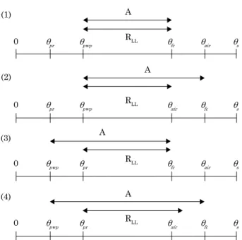
The Least Limiting Water Range (rLL, m3 m-3) is defined as:
rll = max [0, min (θfc, θair) - max (θpwp, θpr)] Eq. 1
where “max” represents the “maximum” function (max(i,j) = i if i≥j; max(i,j) = j if i<j), and “min” is the “minimum” function (min(i,j) = i if i≤j; min(i,j) = j if i>j). The definition of rll includes four limiting
soil water contents, all on a volume base (m3 m-3): θfc is the water content at field capacity; θair, is the
limiting water content for proper aeration; θpwp is the water content at the permanent wilting point; and θpr, is the soil water content corresponding to the limiting penetration resistance. The rll indicator can be compared to the quantity available water A (m3 m-3), defined as:
A = max [0, θfc - θpwp] Eq. 2
Figure 1 shows the graphical representation of rll and A, according to equations 1 and 2 for the
four possible combinations of the relative position of θpwp and θpr and of θair and θfc. A will be equal
to rll in the case of θpwp≥θpr and θfc≤θair (case 1, Figure 1). In all other cases, rll will be smaller
than A.
The limiting water contents, their coherence and parametrization
The limiting contents that comprise the rll
definition (Equation 1) are:
• The field capacity limiting water content
rate of downward movement of water has materially decreased, which usually takes place within 2 or 3 days in pervious soils of uniform structure and texture”.
• The limiting water content for proper aeration (θair), which is the maximum water
content corresponding to an air-filled porosity
that allows an adequate exchange of gases between soil and atmosphere, ensuring that in any rooted portion of the soil there is no excess of CO2 or lack of O2. The crop stress associated with this parameter (if θ>θair) is the anoxic stress.
• The limiting water content corresponding to the permanent wilting point (θpwp), which delimits soil conditions in which a plant will permanently (that is, without recovery) wilt in short time. The stress associated with this parameter (if θ<θpwp) is the drought stress.
• The limiting water content related to excess root penetration resistance (θpr), representing the water content below which the plant roots cannot penetrate the soil for mechanical restrictions. The stress associated with this parameter (if θ<θpr) is the mechanical stress.
A cursory analysis of the limiting values that are
used to define rll reveals some key aspects. Two of
the limiting water contents, θpwp and θpr, represent
conditions that correspond to the “fatal” limit of the respective stress - drought and mechanical (permanent wilting and zero root growth), while a third water content, θair, corresponds to the
onset of the anoxic stress phase, when aeration conditions have just begun to cause damage to the plant, but below a fatal stress level. The three types of stress regarding their respective limiting
contents are schematically represented in figure 2. In the example illustrated in this figure, there is a
near-fatal stress condition (water content “1”, where the water content is slightly above θpwp), which,
nevertheless, is within the range considered as rll.
An opposite situation, i.e., water content outside the rll, but without causing stress to the plant,
may occur when θfc<θair (cases 1 and 3 of Figure 1) and when θfc<θ<θair (situation 2, Figure 2). In such
conditions, the plant is not suffering any kind of stress, however, the corresponding water content is not included in the rll. Considering the definition
of field capacity, water contents higher than θfc will
rapidly decrease in time due to drainage, and θfc will be reached in a matter of days. Depending on rainfall and other boundary conditions, the amount of water taken up by the plant in the range of θfc and θair,
when θfc<θair, may, nevertheless, be considerable. In virtually all studies published in Brazil on the subject, the parametrization of the four limiting contents of the rll is fake and just consists of using
a set of fixed values. For θfc a water content is used
that corresponds to a given matric potential (-10 or -33 kPa, in general); θair is chosen to match the
air content of 0.10 m3 m-3; θ
pwp is considered to
correspond to the matric potential of -1,500 kPa; and θpr is chosen equivalent to the water content
at which the soil has a predefined resistance to
penetration (often 2 MPa). Except in some studies (Klein and Camara, 2007; Kaiser et al., 2009; Gubiani et al., 2013b), the values in general are not tested and compared with biological measurements, and a sensitivity analysis of the outcomes of studies regarding these values is rarely performed. In some cases, only the effect of the value chosen for penetration resistance in θpr is assessed (Betioli
Júnior et al., 2012; Moreira et al., 2014b). The
justification for using one or another set of values, if
any, has been limited to quoting other publications
in which the same values were used. The scientific flaw of doing so becomes clear when one realizes
that the cited papers did, on their turn, not present
sustainable justification; the values employed were
chosen by someone at a certain moment, but their validity is much more the product of self-assertion
than experimental scientific confirmation.
Moreover, few studies focus on the association of rll and crop response. Those who do show low
A
RLL (1)
A (2)
A (3)
A (4)
θpr
0 θpwp θfc θair θs
RLL
θpr
0 θpwp θair θfc θs
RLL
θpwp
0 θpr θfc θair θs
RLL
θpwp
0 θpr θair θfc θs
Figure 1. Least Limiting Water Range (rll) and
available water (A) on a scale of volumetric water contents from completely dry (0) to
saturation (θs), according to equations 1
and 2 for the four possible combinations of the relative position of water contents of permanent wilting and limiting root
penetration resistance (θpwp and θpr) and of
correlation, as found in a wide literature review (Gubiani et al., 2013a), as well as in an experimental corroboration with eight maize crop cycles (Gubiani et al., 2013b).
Such apparent contradiction - it would be reasonable to assume that an indicator of soil physical quality applied to agronomy would have correlation with yield - may have two main explanations. There may be a structural problem in the adopted model; in other words, the parameters considered or the way they are related to calculate the rll (Equation 1)
are not sufficient to represent the processes that
determine the crop yield. Alternatively, the calibration of the model may be wrong, i.e. the values attributed to the limiting contents are incorrect.
Taking into account that the parameters included in the calculation of rll can represent drought stress
and anoxic stress, and also include mechanical root growth stress, the most likely explanation for the observed low correlation is the simple way by which the parameters are related in rll as well as
inaccuracies in their calibration.
Limiting contents versus physical properties
In the following, we describe some relationships between the rll limiting water contents and
primary soil physical properties that can be determined objectively.
The field capacity limiting water content versus hydraulic retention and conductivity
Field capacity, by definition, is related to the
vertical water draining movement and, therefore,
depends on the water flow through the soil profile. The water flow in porous media is described by the
Darcy-Buckingham Law, which establishes that the
water flux density is equal to the product of hydraulic
conductivity and the total hydraulic gradient. This law, when combined with the mass conservation principle, results in the Richards Equation, allowing predictions on soil water conditions in time and space. In addition to information on the
specific geometry of the problem, in order to apply
the Richards Equation it is necessary to know the relationship between hydraulic conductivity (K), matric potential (h) and water content (θ). Such relationships are highly nonlinear and hysteretic, and describing them in a mathematical format allowing a relatively simple solution is still one of the challenges of soil physics.
The relation between soil water content or
matric potential at field capacity and soil hydraulic
properties may be assessed simulating an internal drainage experiment using a hydrologic model based on the Richards Equation. Following this approach, Twarakavi et al. (2009) used the Hydrus model (Simunek and van Genuchten, 2008) and estimated
field capacity for a large number of soils, discussing
the sensitivity of the determination to the soil hydraulic properties and the criterion of negligibility of the drainage rate to be adopted. These authors proposed the following empirical equation to
estimate the water content at field capacity as a
function of other soil physical parameters:
θfc = θr + (θs - θr)n0.60log10 qfc
Ks
Eq. 3
where θr, θs and n are parameters of the water
retention equation by van Genuchten (1980); Ks is the saturated hydraulic conductivity and qfc is the
flux considered negligible for the purposes of field
capacity estimation. In this equation, Ks and qfc
should be expressed in the same unit of time per length (TL-1).
By combining equation 3 with the van Genuchten (1980) water retention equation, the following
expression for the matric potential at field capacity
is obtained:
0.60 n log10 qfc
Ks
hfc = α
1 - n
n −1
1
n
Eq. 4
In this equation, hfc assumes the inverse unit of the α parameter from the van Genuchten (1980) equation. For example, if α is chosen in cm-1, hfc will
be in cm. Twarakavi et al. (2009) concluded that the
use of a “negligible” flux of qfc = 0.01 cm d-1 resulted
in good estimations of field capacity for a wide range
of soils; and for this qfc value, equations 3 and 4, for Ks in cm d-1, become, respectively:
θfc = θr + (θs - θr)n-0.60(2 + log10Ks) Eq. 5
hfc = α
0.60 n (2 + log10 Ks)
n - 1
n −1
1
n
Eq. 6
Based on their studies, Twarakavi et al. (2009), similarly to Souza and Reichardt (1996), concluded
that the use of a fixed value for the matric potential
to estimate field capacity does not correspond to reality. Figure 3 shows the hfc values as a function of
θpr
0
RLL
Drought stress Mechanical stress
Anoxic stress 2
1
θpwp θfc θair θs
the saturated hydraulic conductivity Ks, as calculated by equation 6 for soils with α = 0.015 cm-1 and for
five values of parameter n. The figure illustrates the
tendency that is intuitively perceived: higher Ks values
result in quicker drainage, causing the soil to dry more (more negative matric potential) until reaching the draining rate that was pre-established as negligible.
The equation developed by Twarakavi et al. (2009) was included here just as an example. For its development a soil database was used that contains predominantly soils from temperate regions. Moreover, equation 4 does not allow the inclusion of vertical
heterogeneity (stratification) of the soil, which, when
it occurs, may have a major effect on the water content
and on the matric potential corresponding to field
capacity. It would not be possible to include such heterogeneity in a simple empirical equation like equation 4, because it would increase the number of parameters in such a way that a solution by regression, as obtained by Twarakavi et al. (2009), would become inviable. Moreover, applications to solve for the problem of multi-layer systems already exists, in the form of numerical hydrologic models based on the Richards Equation. One of these models (Hydrus) was used by Twarakavi et al. (2009) themselves and depends only on the hydraulic properties as a function
of depth to calculate the flows.
The limiting water content corresponding to the permanent wilting point versus retention and hydraulic conductivity
The water content corresponding to the permanent wilting point (θpwp), by definition, refers to the lower
limit of extractable soil water by plant roots. Its experimental determination is time-consuming and obtained values are discussed, e.g., by haise et al. (1955), Veihmeyer and hendrickson (1955) and Cutford et al. (1991). The soil water content can become lower than θpwp only by evaporation or drainage. Therefore, using θpwp to calculate crop
available water A seems plausible, but its use in the rll definition, with the adjective least limiting,
does not seem reasonable, as will be explained in the following.
The inclusion of θpwp in rll as the lower limit corresponding to drought stress represents a gross simplification of the existing knowledge on transpiration reduction due to soil drying, as observed in experiments like those reported by Meyer and Green (1980), Wright and Smith (1983), Casaroli et al. (2010) and many others. To improve the empirical modeling of this phenomenon, Doorenbos and Kassam (1986), Feddes et al. (1978, 1988) and van Genuchten ( 1 9 8 7 ) d e v e l o p e d m a t h e m a t i c a l l y s i m p l e proposals to describe the phenomenon, used in several hydrological models, such as Hydrus and SWAP. Lascano and van Bavel (1986), Jarvis (1989, 2011) and Li et al. (2001) offered relatively simple proposals that allow considering the soil vertical heterogeneity as well.
The permanent wilting water content θpwp is
defined based on the process of water uptake by
plant roots; to predict it, one should model the water
flow towards the plant roots, which, in the same
way as for θfc, can be done by means of the Richards equation with appropriate boundary conditions. Classical publications on the item are those by Gardner (1960) and Cowan (1965) who developed theories based on the Richards equation and basic theory of water extraction from the soil by the plants.
Numerical algorithms based on the theory by Gardner (1960) were presented in several recent publications (Javaux et al., 2008, 2013; De Jong van Lier et al., 2006, 2013; Couvreur et al., 2012). The
plant root geometry and properties, specifically the
limiting root (or leaf) water potential and internal plant resistances, together with the soil water potential and the hydraulic conductivity of the soil near the roots, determine whether a plant can or cannot withdraw water at rates compatible with the atmospheric demand, allowing the assessment of drought stress.
Consequently, regarding the lower limit for crop water availability, retention and hydraulic conductivity are the physical properties of major interest. De Jong van Lier et al. (2006, 2008) showed
that the matric flux potential (m, m2 d-1) (Gardner,
1958; Raats, 1970; Pullan, 1990), a soil physical property that integrates retention and conductivity, is the physical parameter most directly linked to crop available water. m is defined as:
10 100 1,000
0.1 1 10 100 1,000
Matric potential at field capacity,
hfc
(-cm)
Saturated hydraulic conductivity, Ks (cm d
-1)
n = 4
n = 3
n = 2
n = 1.5
n = 1.2
Figure 3. Matric potential corresponding to field capacity (hfc) as a function of saturated hydraulic conductivity (Ks), according to Twarakavi et al. (2009) (Equation 6) considering a negligible bottom flux for the purpose of field capacity (qfc) of 0.01 cm d-1, for five van Genuchten (1980) soils (five values of shape factor n; shape factor α equal to
m = ∫K (h)dh h
hl Eq. 7
where hl is the limiting matric potential, the most negative value that the water in the roots can assume. By writing the Darcy equation in terms of m it is shown that the spatial gradient of m (dm/dx)
is equal to the water flux density in the absence of gravitational flow, which, approximately, is the case
for water uptake from the soil by plant roots. W h e n t h e K(h) f u n c t i o n i s k n o w n , t h e determination of M(h) is a matter of analytical or numerical integration. Figure 4 illustrates, for two differently textured soils, hydraulic conductivity K
(Figure 4a) and its integral, the matric flux potential
m (Figure 4b) as calculated by equation 7, as a function of the matric potential. For a given matric potential, the m value corresponds to the ease with which a plant withdraws water from the soil. Figure 4c shows the ratio of the m values of the two soils as a function of the matric potential. It can be seen that for not too negative matric potentials (wet soil), the relative difference between the m values for both soils is small, but for more negative matric potentials (drier soil) the m of the clay loam soil becomes orders
of magnitude higher than in the sandy loam soil. This indicates a much higher availability of water in the clay loam soil.
The limiting water content for proper aeration versus gas diffusion
Soil aeration is the process through which the gases produced or consumed in soil are exchanged with the atmosphere, primarily by diffusion. The main gas consumed in the soil is oxygen, whereas the main gas produced is carbon dioxide. Thus,
soil aerobic processes depend on the flow of O2
from the atmosphere into the soil, and of CO2 in the opposite direction. Diffusion of these gases is much higher in air than in water. So, the higher
the soil water content the greater the difficulty
for an adequate aeration, which can hinder plant growth and should be considered for the modeling of plant production.
By integrating various factors that control the aeration process in order to meet the biological demand, as described by De Jong van Lier (2001), De Jong van Lier and Cichota (2004) presented the following equation to estimate the minimum
1 10 100
1 10 100 1,000 10,000
M
clay loam
/
M
sandy loam
(c)
Matric potential, h (-cm)
Matric potential, h (-cm)
1 10 100 1,000
1 10 100 1,000 10,000
Matric flux potential,
M
(cm
2 d -1)
sandy loam
clay loam (b)
1 10 100 1000 10,000 100,000
Hydraulic conductivity,
K
(μm d
-1)
Matric potential, h (-cm)
sandy loam
clay loam
10-3
10-1
10
103
105
(a)
Figure 4. Hydraulic conductivity K (a), the matric flux potential M (b) (integral as calculated by equation
required aeration porosity as a function of the O2 consumption in the soil, the depth and total porosity of soil, the O2 content in the atmosphere and O2 diffusion in the air:
βmin = SmaxZ
2χ2 p
([o2]atm - [o2]min)dα 2p + 4
¾10
Eq. 8
In this equation, βmin (m3 m-3) is the minimum
aeration porosity necessary to ensure that no part of the plant root system will suffer from lack of oxygen; Smax (kg m-3 s-1) is the oxygen consumption
rate per unit of soil volume at the soil surface (Smax
was considered as 28.2∙10-8 kg m-3 s-1); Z(m) is the
rooting depth; χ (m3 m-3) is total porosity (χ was
considered equal to 0.5 m3 m-3); [O
2]atm (kg m-3), the
oxygen concentration in atmosphere, considered as 0.269 kg m-3; [O
2]min (kg m-3) is the minimum oxygen
concentration to sustain life at a given soil depth (considered [O2]min equal to [O2]atm/4); da (m2 s-1) is
air diffusivity for oxygen (da= 1.78∙10-5 m2 s-1); and
p is a factor determining the shape of the function of O2 consumption decrease with depth (SO2, kg m-3 s-1)
(De Jong van Lier and Cichota, 2004), where SO2 is
equal to Smax at the surface (z = 0) and zero when
z = Z, according to:
SO2 = Smax 1 -p z
Z
Eq. 9
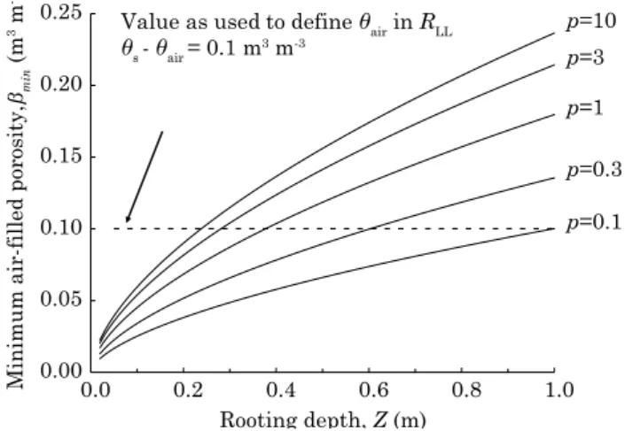
Equation 8 was applied for rooting depths up to 1.0 m and for p-values of equation 9 that represent different oxygen consumption distributions with depth, from consumption concentrated at the soil surface (p=0.1) to a practically equal consumption at all depths occupied by the root system (p=10) (Figure 5). As a result, βmin ranged from 0.02 to 0.24 m3 m-3. This range could be enlarged
considering other values for χ and Smax. It is worth noting that the βmin values, as calculated by equation
8 and represented in figure 5 refer to the minimum
air content at the soil surface, through which all O2 consumed and CO2 produced in the soil profile is
flowing. The greater the depth, the smaller the flow
of O2 and CO2 and the smaller will be the content
of air required for an adequate aeration. Clearly,
the application of any fixed value for βmin, such as
the value of 0.1 m3 m-3 used for calculation of θ
air of
rll,means failing to consider the complexity of the
aeration process and believing that it is possible to
infer biological consequences from a fixed fraction
of soil porosity not occupied by water.
A more complete approach of the subject is presented by Bartholomeus et al. (2008), who modeled, besides the soil macroscopic diffusion, the microscopic oxygenation process of individual roots, and found βmin values varying from 0.02 and 0.08 m3 m-3 for diverse scenarios, together with a
high sensitivity for soil temperature and rooting
depth. According to these authors, fixed values
for βmin (such as the 0.1 m3 m-3 value adopted in
virtually all works involving rll) very unlikely will
represent an approximate value of the actual value.
The limiting water content related to penetration resistance versus the physics of root elongation
The resistance that solid particles in the soil apply against a motion or displacement results from complex relations of cohesive forces of solid-solid interactions, adhesive forces of solid-liquid interactions and frictional forces generated during displacement (Keller et al., 2013). When a root penetrates the pores of a soil,
its growth will cause a significant displacement of
the particles when it does not change its geometry
to fit the irregular geometry of the pore space,
when it forces its way through the pore cavity that
it had filled or when pore space must be created
(Bengough et al., 1997, 2006, 2011; Clark et al., 2003). Root growth can be considered a cell mass
flow into the soil (cell division and elongation). Directing the cell flow to less resistant areas is a
biological strategy to save the energy captured in the photosynthesis process.
The Lockhart’s model (Lockhart, 1965; Jordan and Dumais, 2010), employed in plant physiology to study the force relations involved in cell elongation,
considers that cell walls behave as a Bingham fluid. A Bingham fluid, as opposed to a Newtonian fluid,
requires a minimum pressure σY>0 to cause its
deformation. The relative deformation rate over time will be proportional to the applied pressure σ (Pa) reduced by σY (Pa):
= μ[σ - σY]
1dl
l dt Eq. 10
where l (m) represents the root length, t (s) is time, and the property μ (Pa-1 s-1) is called extensibility.
In the case of cell elongation, σY can be understood
0.00 0.05 0.10 0.15 0.20 0.25
0.0 0.2 0.4 0.6 0.8 1.0
Minimum air-filled porosity,
βmin
(m
3 m -3)
Rooting depth, Z (m)
p=0.1 p=10
p=3
p=1
p=0.3 Value as used to define θair in RLL
θs - θair = 0.1 m3 m-3
Figure 5. Minimum air-filled porosity for proper
aeration βmin as a function of the empirical parameter p and depth of the root system Z, as
as the cell wall resistance (r, Pa), i.e. the pressure at which the cell walls resist deformation. The cell turgor (T, Pa) is the internal cell pressure and is equivalent to the σ of equation 10 (Bengough et al., 1997). The difference between T and r is called net cell pressure (Plc, Pa):
Plc = T - R Eq. 11
By comparing equations 10 and 11, we see that Plc represents the rate of deformation over time divided by its extensibility.
The soil mechanical resistance to root growth effectively occurs only when turgid roots exert pressure on the surrounding environment. In these cases a reaction pressure (Prs) is produced by the
soil, its value being limited to the soil mechanical impedance Prs,max. The direction of the resulting force from such pressure in the cell wall is opposite to the force provided by the cell turgor pressure (Plc). The roots continue growing and moving soil particles while Plc>Prs,max. Note that the presence of roots is indispensable for the existence of Prs, but
their presence alone is not sufficient, because those
roots with Plc=0 do not provide the required physical conditions for the occurrence of Prs.
Quantification of the soil mechanical impedance
can be achieved by using available types of penetrometers and measurement techniques, as discussed by Stolf (1991). In general, the soil mechanical impedance measured by penetrometers (rP, Pa) is the quantification of the soil response to pressure, resulting from the reaction to the pressure caused by the penetration of a metal cone positioned at the end of a rod into the soil. Although rP is useful
to detect differences in soil resistance as a function of cohesive, adhesive or frictional forces and to distinguish pedological and tillage factors that affect such forces, it will not represent the manifestation of Prs, given the physical conditions required for the
occurrence of Prs and because of the different scales and geometries of the cell expansion when compared to the penetrometer cone.
Because of the difficulty in determining Prs,max, some researchers attempted to establish empirical relationships between rP and the cell elongation rate dl/dt. In a recent literature review, some relationships were presented and discussed by Bengough et al. (2011). From their experiments it became evident that in order to obtain empirical relations a homogeneous soil matrix (samples prepared in laboratory) was a prerequisite, as well as matric potentials less negative than -0.5 to -0.1 MPa. In the same moist conditions, the expectation is that the relation between dl/dt and rP will not
be confirmed in cases where cracks and biopores
are present, occupying a large portion of the soil
volume (the plant directs the cell flow to less
resistant spaces) which is common in conservation-tillage crop areas (Ehlers et al., 1983). For such
areas and based on the criterion that there has not been a close relationship between some biological variable with rP, some researchers suggest that critical rP values should be higher than 2 MPa
(Klein and Camara, 2007; Reichert et al., 2009; Moraes et al., 2014). however, the use of values above 2 MPa (e.g. 3.5 MPa as suggested by Moraes et al., 2014) often corresponds to matric potentials close to the permanent wilting point. In some cases of the study conducted by Moraes et al. (2014), rP would reach 3.5 MPa only for
matric potentials below the wilting point. In such conditions, Plc and, consequently, Prs, can be so
small that the biological stress associated with the mechanical factor is negligible if compared to the stress associated with the drought factor. In these cases, interpreting the occurrence of loss in biological variables as caused by a high rP means the incorrect attribution of the cause
to the mechanical factor when it is essentially a lack of water.
The empirical relationships established between rP and other soil properties, such as those used to
estimate rP as a function of bulk density (ρ) and
water content [rP = f (ρ, θ)], and which constitute the mathematical sub-model of the limiting mechanical impedance often used in combination with the calculation of rll, are useful to represent
the relationship between the soil properties included in the sub-model. however, such models of relationships between soil properties do not contain any information about the occurrence and magnitude of Prs. Its use in the context of rll aiming to estimate θpr corresponding to a fixed rP
only informs that the mechanical reaction of soil to a metal rod, in terms of pressure, would be equal to
the fixed rP value. Assuming that the roots face this
same resistance means accepting all interpretation errors of the cause factor and the conceptual errors previously mentioned.
Problems and mistakes in interpreting the RLL
Interpretation of rll values is achieved by comparison. It is often concluded that the soil physical quality worsened when the rll decreased
as a function of some agricultural tillage system or other factor. Such comparison usually includes an assessment of different scenarios. Changes in soil management, for example, represent changes in the plant root density, rooting depth, and soil hydraulic properties. At the same time, the rll in its original
conception has limitations when the scenario presents more complex boundary conditions. Is it
plausible to use fixed values for the limiting contents
Then, how could the rll be used as an indicator? According to the previous discussion, it would be necessary to estimate the limiting contents considering the changing boundary conditions. This process would be as complex, or even more complex, than the use of a detailed mechanistic model and, therefore, the advantage of rll being a “simple” indicator would disappear.
Regarding the upper limit of the rll, the inconsistencies in the choice of θair or θfc as limiting
values have already been discussed. For the lower limit, it was observed that θpwp corresponds to a condition of total drought stress, which would better be replaced by a value corresponding to a considerable stress, but not total, or, in analogy to what is done in the case of θair, to the water content
corresponding to the onset of drought stress. The relationship between drought stress and matric potential is discussed in detail by Metselaar and De Jong van Lier (2007) and by De Jong van Lier et al. (2009). The theory presented in these publications
shows that drought stress, quantified by relative
transpiration, increases in a nonlinear way when the matric potential decreases from a certain value, generally in the range of -30 to -100 kPa (Kukal et al., 2005; Liu et al., 2012), much less negative than the permanent wilting point. Thus, the use of a water content corresponding to this order of magnitude of potential (critical water content,
θcr) to replace θpwp in the calculation of the rll
sounds reasonable and was proposed yet recently by Silva et al. (2015). Their data show that, as a consequence, the permanence of θpr in the rll
calculation would be superfluous, once its value,
in almost all situations, would be lower than θcr.
This finding corroborates with the fact that the
major models of plant growth do not use, among their input data, information on the penetration resistance, and yet they result in good predictions. Apparently, the process (plant growth) is not sensitive to parameters that relate penetration resistance to water content.
Two boundary conditions, common in numerous production systems, will be discussed in the following
sections. The first refers to the phenology of the crop
under observation; the second, to variations in soil properties with depth. For neither of them rll can be easily introduced as an indicator.
Phenological boundary conditions and their consequences for the RLL
During crop development, plants undergo a series of phenological changes that affect the transfer of mass and energy in the soil-plant-atmosphere system. The most obvious parameters include changes in the rooting depth, distribution and growth, leaf area index, carbohydrate partitioning among plant organs and other physiological parameters. hydrological models, when coupled
to plants growth models, usually treat these parameters as a function of time, development stage or accumulated heat sum. For the purpose of rll, interpretation would be achieved based on
the limiting contents that, except for θfc, which is exclusively related to soil, should be considered as variable during crop development.
As the rooting depth and root length density increase, βmin increases and the corresponding θair
decreases. Thus, for the first phenological stage, the required air-filled porosity is very low and θair
becomes virtually equal to θs; at the peak of root growth, according to the theory presented, βmin can represent half of the total porosity (Figure 5). The great variation of these values during the cycle of an annual crop shows that the use of a rll with
fixed limiting values is not consistent with the real
conditions in this context either.
Regarding θpr, in the reproductive stage
root growth becomes irrelevant. hence, in this phenological stage, the mechanical resistance is no longer biologically important, θpr equals zero, and
the expression to calculate rll (Equation 1) could
be reduced to:
rll = max [0, min (θfc, θair) - θpwp] Eq. 12
This fact is important, for example, when assessing the correlation between grain productivity and rll, which may show a significant reduction of
rll if θpr is the lower limit of rll and θpwp<θ<θpr, but this reduction is not correlated to dry matter accumulation during the reproductive phase.
The value of θpwp (or the critical water content
θcr that might replace it) should also be dependent
on crop phenology. As previously discussed, θpwp is
influenced by the root system's ability to withdraw a sufficient amount of water from the soil to meet
the transpiration demand. The transpiration demand is determined, among other factors, by the leaf area index, which is dependent on development stage. Simultaneous with an increase in leaf area, the root system also grows in depth and density. The combined effect of these factors should be considered for an accurate determination of the value of θpwp or θcr.
Pedological boundary conditions and their consequences for the RLL
Most soils present morphological stratification.
The distribution of the root system in the soil, with a density that normally decreases with
depth, superposes this pedological stratification.
indicator, its definition is applicable to only one soil
horizon, however, scenarios in which the conditions of one horizon are outside the rll, while another
horizon is within rll may be supposed to occur frequently. In these cases, the indicator does not allow a unique prediction. To what extent would the favorable conditions in one horizon compensate the unfavorable conditions in another one?
Considering available water A, the integration of its value along the rooted soil depth ze (m) results in
the available water capacity cAW (m):
cAW = ∫Adz
Ze
0 Eq. 13
A similar integration could be proposed for the rll, but it would not make much sense once the
purpose of rll is its use as an indicator of soil
quality. A simple integration, as in the case of cAW, would disregard any compensatory effect that may exist when one soil horizon is outside the optimum range and another one is within it.
Critical density
Very common in publications addressing the least limiting water range is its estimation for several soil densities or degrees of compaction, aiming to predict the effects of a possible compaction on the soil physical quality and crop yields (Imhoff et al., 2001; Leão et al., 2004; Beutler et al., 2008; Blainski et al., 2009; Kaiser et al., 2009; Petean et al., 2010; De Lima et al., 2012; Farias et al., 2013; Guimarães et al., 2013; Moreira et al., 2014a; Seben Junior et al., 2014). In this case, θfc and θpwp are
usually estimated as a function of an empirical relationship between the water content, bulk density and matric potential proposed by Silva et al. (1994) or other also empirical equations (Guimarães et al., 2013), using fixed values for the matric potential; θpr is calculated as a function of soil bulk
density using the empirical model proposed by
Busscher (1990), assessing it for a fixed impedance
value, commonly 2 MPa; and θair is calculated by
subtracting 0.1 m3 m-3 from total porosity, which is
a function of the bulk and particle density.
The results are usually presented in the form of a graph of the four limiting water content values, where the abscissa represents the soil bulk density and the ordinate represents the water content, as
exemplified in figure 6. In this context, “critical bulk density” is defined as the lowest soil density
for which the rll equals zero. For such bulk density, or higher values, irrespective of the water content in the soil, it would be outside the rll,
and, therefore, productivities in such soils would always be reduced.
The described procedure is emblematic for the shift of attention that resulted from the introduction of the rll in Brazilian scientific circles. The
processes and mechanisms that govern the system
are not discussed. Instead, conclusions are based on the perfection attributed to the indicator. To its value, obtained by extrapolation of experimental observations using empirical relationships, predictive qualities and recommendations on soil management to establish required bulk densities are attributed. however, it is clear that, in case of soil compaction (a decrease in total porosity, particularly in macroporosity), there are predictable changes for almost all soil physical properties. Such changes will
influence the rll limiting contents in an equally
predictable manner, as exemplified by the dotted lines in figure 6 and detailed as follows:
a. The saturated or near-saturated hydraulic conductivity decreases as macroporosity decreases. hence, the draining process
slows down, and the water content at field
capacity (dependent on the negligibility criterion) will correspond to a less negative matric potential (wetter soil) than for the same non-compacted soil, as also discussed in the context of the equation 6 developed by Twarakavi et al. (2009).
b. By reducing total porosity, according to De Jong van Lier (2001) and Bartholomeus et al.
(2008), the minimum air-filled porosity is
expected to decrease. Taking into account that compaction is likely to cause a reduction of the root growth as well as of the depth of the soil explored by the root system, the
minimum air-filled porosity would be even
more reduced. For example, using the values presented by De Jong van Lier (2010) for high oxygen consumption conditions, if total porosity decreases from 0.6 to 0.5 m3 m-3 and
the depth of the root system decreases from
0.5 to 0.4 m, the minimum air-filled porosity
would decrease from 0.17 to 0.13 m3 m-3.
c. Compaction reduces the soil hydraulic conductivity at high water contents, but increases the hydraulic conductivity under drier conditions (hillel, 2003). Thus, in drier soils, access to water will be easier in compressed soil, and the matric potential corresponding to θpwp or θcr is expected to decrease (become more negative).
These predictable facts show the non-validity of
fixed values of air content and matric potentials for
calculation of the rll limiting contents when the
objective is to compare its value before and after a compaction. As rll assessment is always made with
fixed values to assess the limiting levels, whereas
FInAL COnSIDERATIOnS
Considering the availability of robust models for agronomy, ecology, hydrology, meteorology and other related areas, the appeal of the rll as an indicator
in Brazilian soil physics cannot be assumed for its effectiveness, never proven, but should be explained by the simplicity with which it is dealt. The exercise of estimating the limiting water contents in the light of the state of the art of soil physics, instead of considering them a function of simple constants, proves to be as or more complex than the existing mechanistic models. The amount and extent of objective information contained in the rll limiting contents, when based on constants, is minimal when compared to the amount of objective information contained in continuous functions of properties of biological and physical processes. Thus, the great disadvantage of using the rll as an indicator
compared to the use of models that integrate such functions based on mechanistic knowledge becomes evident. The rll is a mathematical model, but a
sensitivity analysis of rll to the limiting values was
only performed in one of the first publications on
the subject (Silva et al., 1994). Since then, what has been done as an approximation of calibration is not much more than verifying the dependence between rll and the soil bulk density. The few tests of the
correlation between rll and crop yields, as described
by Gubiani et al. (2013a), in most cases refuted it, as also reported by Gubiani et al. (2013b). Further research conducted with the purpose of revealing the
relationship between rll and soil bulk density or compaction, without questioning the limiting values or testing the sensitivity of rll to these values will not add knowledge and should be discouraged. Research on rll can provide scientific contribution,
but should inform in which circumstance rll is a
reliable indicator of the soil physical quality for plant production by comparing plant variables with water content in the context of rll.
COnCLUSIOnS
The four limiting contents of the rll are related
to crop yield. however, their determination using
fixed values of air content, matric potentials and
mechanical impedance of soil marginalizes the
existing knowledge in the field of soil physics, plant
physiology and agrometeorology.
When calculated using the limiting water content for the onset of drought stress instead of the permanent wilting point, rll shows insensitive
to parameters that relate penetration resistance to water content. This corroborates to the fact that major crop growth and yield prediction models do not include soil mechanical information among their input parameters, and suggests that the determination of these parameters in the context of soil water availability and crop growth is counterproductive.
The search for quantifying concepts such as the least limiting water range rll goes against the
systemic understanding, being restricted to the simple determination of the respective limiting values, relegating the study or concern with the actual functioning of the system to a secondary role. Contrary to more complex models, indicators such as the rll, with fixed limiting values as most
researchers use them, show no correlation with crop productivity.
In the light of such findings, the attention given
to the rll in Brazilian soil physics is not justified.
The authors of this study suggest a realignment of the research in Brazilian soil physics with the scientific principles towards emphasizing mechanistic soil physics rather than the search for empirical correlations far below the state of the art of soil physics.
REFEREnCES
Abdelhafeez AT, harssema h, Verkerk K. Effects of air temperature, soil temperature and soil moisture on growth and development of tomato itself and grafted on its own and egg-plant rootstock. Sci hortic. 1975;3:65-73.
Wa
te
r conten
t
Bulk density θpwp
θpr
“critical” density θfc
θs = 1 - ρ/ρs
θair = 1 - ρ/ρs - 0.1
Figure 6. Representation of RLL limiting water
contents versus bulk density. Solid lines
represent the limiting water contents of RLL estimated based on fixed parameters; dotted lines show the expected behavior of the limiting water contents based on physical knowledge. The gray colored area represents the RLL integral over the range of represented densities. θpwpθfc,
Allen RG, Pereira LS, Raes DE, Smith M. Crop evapotranspiration: Guidelines for computing crop water requirements. Rome: FAO; 1998. (Irrigation and Drainage Paper, 56).
Arnold JG, Moriasi DN, Gassman PW, Abbaspour KC, White MJ, Srinivasan R, Santhi C, harmel RD, Van Griensven A, Van Liew MW, Kannan N, Jha MK. SWAT: Model use, calibration, and validation. Trans Am Soc Agric Biol Eng. 2012;55:1491-508. Bartholomeus RP, Witte JM, Van Bodegom PM, Van Dam JC, Aerts R. Critical soil conditions for oxygen stress to plant roots: Substituting the Feddes-function by a process-based model. J hydrol. 2008;360:147-65.
Bengough AG, Bransby MF, hans J, Mckenna SJ, Roberts TJ, Valentine TA. Root responses to soil physical conditions; growth
dynamics from field to cell. J Exp Bot. 2006;57:437-47.
Bengough AG, Croser C, Pritchard J. A biophysical analysis of root growth under mechanical stress. Plant Soil. 1997;189:155-64. Bengough AG, Mckenzie BM, hallett PD, Valentine TA. Root elongation, water stress, and mechanical impedance: a review
of limiting stresses and beneficial root tip traits. J Exp Bot.
2011;62:59-68.
Betioli Júnior E, Moreira Wh, Tormena CA, Ferreira CJB, Silva AP, Giarola NFB. Intervalo hídrico ótimo e grau de compactação de um Latossolo Vermelho após 30 anos sob plantio direto. R Bras Ci Solo. 2012;36:971-82.
Beutler AN, Centurion JF, Silva AP, Centurion MAPC, Leonel
CL, Freddi OS. Soil compaction by machine traffic and least
limiting water range related to soybean yield. Pesq Agropec Bras. 2008;43:1591-600.
Blainski E, Gonçalves ACA; Tormena CA, Folegatti MV, Guimarães RML. Intervalo hídrico ótimo num Nitossolo Vermelho distroférrico irrigado. R Bras Ci Solo. 2009;33:273-81.
Busscher WJ. Adjustment of flat-tipped penetrometer resistance
data to a common water content. Trans Am Soc Agron Eng. 1990;33:519-24.
Casaroli D, De Jong van Lier Q, Dourado Neto D. Validation of a root water uptake model to estimate transpiration constraints. Agric Water Manage. 2010;97:1382-8.
Clark LJ, Whalley WR, Barraclough PB. how do roots penetrate strong soil? Plant Soil. 2003;255:93-104.
Couvreur V, Vanderborght J, Javaux M. A simple three-dimensional macroscopic root water uptake model based on the hydraulic architecture approach. hydrol Earth Syst Sci. 2012;16:2957-71. Cowan IR. Transport of water in the soil-plant-atmosphere system. J Appl Ecol. 1965;2:221-39.
Cutford hW, Jefferson PG, Campbell CA. Lower limit of available water for three plant species grown on a medium-textured soil in southwestern Saskatchewan. Can J Soil Sci. 1991;71:247-52. De Jong van Lier Q, Cichota R. Modelagem da aerabilidade do solo. In: Anais da 15ª Reunião Brasileira de Manejo e Conservação do Solo e da Água; 2001; Santa Maria. Santa Maria: Sociedade Brasileira de Ciência do Solo; 2004. v.1.
De Jong van Lier Q. Disponibilidade de água às plantas. In: De Jong van Lier Q, editor. Física do solo. Viçosa, MG: Sociedade Brasileira de Ciência do Solo; 2010. p.283-98.
De Jong van Lier Q. Oxigenação do sistema radicular: uma abordagem física. R Bras Ci Solo. 2001;25:233-8.
De Jong van Lier Q. Revisiting the S-index for soil physical quality and its use in Brazil. R Bras Ci Solo. 2014;38:1-10.
De Jong van Lier Q, Dourado Neto D, Metselaar K. Modeling of transpiration reduction in Van Genuchten–Mualem type soils. Water Res Res. 2009;45:W02422. doi:10.1029/2008WR006938 De Jong van Lier Q, Metselaar K, Van Dam JC. Root water extraction and limiting soil hydraulic conditions estimated by numerical simulation. Vadose Zone J. 2006;5:1264-77.
De Jong van Lier Q, Van Dam JC, Durigon A, Santos MA,
Metselaar K. Modeling water potentials and flows in the soil-plant
system comparing hydraulic resistances and transpiration reduction functions. Vadose Zone J. 2013;12:1-20.
De Jong van Lier Q, Van Dam JC, Metselaar K, De Jong R, Duijnisveld WhM. Macroscopic root water uptake distribution using
a matric flux potential approach. Vadose Zone J. 2008;7:1065-78.
De Lima CLR, Miola ECC, Timm LC, Pauletto EA, Silva AP. Soil compressibility and least limiting water range of a constructed soil under cover crops after coal mining in Southern Brazil. Soil Till Res. 2012;124:190-5.
Dexter AR. Soil physical quality: Part I. Theory, effects of soil texture, density, and organic matter, and effects on root growth. Geoderma. 2004;120:201-14.
Doorenbos J, Kassam Ah. yield response to water. Rome: FAO; 1986. (FAO Irrigation and Drainage Paper, 33).
Ehlers W, Köpke U, hesse F, Böhm W. Penetration resistance and growth root of oats in tilled and untilled loess soil. Soil Till Res. 1983;3:261-75.
Farias IL, Pacheco EP, Viégas PRA. Characterisation of the optimal hydric interval for a yellow Argisol cultivated with sugarcane on the coastal plains of Alagoas, Brazil. R Ci Agron. 2013;44:669-75.
Feddes RA, Kowalik PL, Zaradny H, editors. Simulation of field
water use and crop yield. New york: John Wiley & Sons; 1978. Feddes RA, Kabat P, Van Bakel PJT, Bronswijk JJB, halbertsma J. Modelling soil water dynamics in the unsaturated zone - state of the art. J hydrol. 1988;100:69-111.
Gardner WR. Dynamic aspects of water availability to plants. Soil Sci. 1960;89:63-7.
Gardner WR. Some steady-state solutions of the unsaturated
moisture flow equation with application to evaporation from a
water table. Soil Sci. 1958;85:228-32.
Gilley JE, Doran JW, Eghball B. Tillage and fallow effects on selected soil quality characteristics of former conservation reserve program sites. J Soil Water Conserv. 2001;56:126-32.
Gubiani PI, Goulart RZ, Reichert JM, Reinert DJ. Crescimento e produção de milho associados com o intervalo hídrico ótimo. R Bras Ci Solo. 2013b;37:1502-11.
G u b i a n i P I , R e i c h e r t J M , R e i n e r t D J . I n d i c a d o r e s hídrico-mecânicos de compactação do solo e crescimento de plantas. R Bras Ci Solo. 2013a;37:1-10.
Guimarães RML, Tormena CA, Blainski E, Fidalski J. Intervalo hídrico ótimo para avaliação da degradação física do solo. R Bras Ci Solo. 2013;37:1512-21.