www.hydrol-earth-syst-sci.net/18/4189/2014/ doi:10.5194/hess-18-4189-2014
© Author(s) 2014. CC Attribution 3.0 License.
Effect of parameter choice in root water uptake models – the
arrangement of root hydraulic properties within the root
architecture affects dynamics and efficiency of root water uptake
M. Bechmann1, C. Schneider2, A. Carminati3, D. Vetterlein4, S. Attinger2, and A. Hildebrandt1,5 1Friedrich Schiller University, Jena, Germany, Institute of Geosciences, Burgweg 11, 07749 Jena, Germany 2Helmholtz Centre for Environmental Research, Leipzig, Germany, Department Computational Hydrosystems, Permoser Straße 15, 04318 Leipzig, Germany
3Georg August University, Göttingen, Germany, Faculty of Agricultural Sciences, Department of Crop Sciences, Büsgenweg 2, 37077 Göttingen, Germany
4Helmholtz Centre for Environmental Research, Halle, Germany, Department of Soil Physics, Theodor-Lieser-Strasse 4, 06120 Halle/Saale, Germany
5Max Planck Institute for Biogeochemistry, Jena, Germany, Hans-Knöll-Str. 10, 07745 Jena, Germany
Correspondence to:M. Bechmann ([email protected])
Received: 3 December 2013 – Published in Hydrol. Earth Syst. Sci. Discuss.: 15 January 2014 Revised: 3 September 2014 – Accepted: 5 September 2014 – Published: 27 October 2014
Abstract. Detailed three-dimensional models of root water uptake have become increasingly popular for investigating the process of root water uptake. However, they suffer from a lack of information on important parameters, particularly on the spatial distribution of root axial and radial conductivi-ties, which vary greatly along a root system. In this paper we explore how the arrangement of those root hydraulic prop-erties and branching within the root system affects modelled uptake dynamics, xylem water potential and the efficiency of root water uptake. We first apply a simple model to illustrate the mechanisms at the scale of single roots. By using two ef-ficiency indices based on (i) the collar xylem potential (“ef-fort”) and (ii) the integral amount of unstressed root water uptake (“water yield”), we show that an optimal root length emerges, depending on the ratio between roots axial and ra-dial conductivity. Young roots with high capacity for rara-dial uptake are only efficient when they are short. Branching, in combination with mature transport roots, enables soil explo-ration and substantially increases active young root length at low collar potentials. Second, we investigate how this shapes uptake dynamics at the plant scale using a comprehensive three-dimensional root water uptake model. Plant-scale dy-namics, such as the average uptake depth of entire root sys-tems, were only minimally influenced by the hydraulic
1 Introduction
Soil–plant interactions are important factors in hydrological and ecological processes. By using soil water for transpira-tion, plants are the essential link in the mass and energy trans-fer at the soil–vegetation–atmosphere interface (Shukla and Mintz, 1982). Much of this interaction hinges upon the abil-ity of plants to gain flexible access to soil water (Churkina and Running, 1998; Kleidon and Heimann, 2000; Feddes et al., 2001; Hildebrandt and Eltahir, 2007; Collins and Bras, 2007; Katul et al., 2012). Inversely, changes in soil water content reflect on energy partitioning and carbon fluxes at the soil surface (Kleidon and Heimann, 1998; El Maayar et al., 2009; Seneviratne et al., 2010). Furthermore, access to soil water is an important prerequisite for biomass produc-tion, including crops (Blum, 1996; Huszár et al., 1998; Cai et al., 2009).
The ubiquitous influence of root water uptake on eco-logical and atmospheric processes necessitates the appropri-ate predictionof root wappropri-ater uptake (Shukla and Mintz, 1982; Jackson et al., 2000). For this, together with observations, models have become vital tools that are used both in order to gain local process understanding as well as to predict macro-scopic root water uptake characteristics.
Water uptake is driven by gradients in water potential, whereby water is pulled up from the soil into the root and up to the leaf (Steudle, 2001; Angeles et al., 2004). Besides soil hydraulic resistance, root tissue resistances determine the actual values of water uptake and water transport (Van Den Honert, 1948): radial resistance of soil and roots for the flow path across the soil–root interface and roots axial resistance for the flow path within the root xylem. The ratio between radial and axial resistance is of substantial importance. It shapes the distribution of xylem water potential throughout the root and thus influences root water uptake (Landsberg and Fowkes, 1978). Moreover, Zwieniecki et al. (2003) mod-elled a trade-off between hydraulically active root length and the corresponding water uptake in unlimited water reservoirs. The term “hydraulically active” corresponds to the portion of the root that considerably contributes to root water up-take. The proposed trade-off hinges upon the ratio of radial and axial root hydraulic resistance: when radial resistance in-creases, the active root length inin-creases, whereas water up-take decreases.
For process studies of root water uptake, models that com-pute microscopic three-dimensional root water uptake with respect to gradients in water potential and hydraulic resis-tances have become more and more popular (Clausnitzer and Hopmans, 1994; Tuzet et al., 2003; Doussan et al., 2006; Javaux et al., 2008; Schneider et al., 2010). Most of these models solve water flow equations within the soil and the root system architecture at the same time. They account for the microscopic soil water flow towards individual roots, ra-dial flow into the root xylem and the axial flow within the root xylem. The modelling scale of these process based
ap-proaches comes close to the scale at which actual root water uptake takes place. Thus, they promise an important contri-bution to process understanding. Indeed, they capture well-observed processes such as redistribution of root water up-take due to local limitations of soil water availability, in-cluding moving uptake fronts (Garrigues et al., 2006; Javaux et al., 2008; Schneider et al., 2010) and also hydraulic lift (Dunbabin et al., 2013). This is a major improvement com-pared to empirical models (Feddes et al., 1978). The inherent redistribution of root water uptake based on explicit calcula-tions of water flow in roots is also reported to be superior to qualitative approaches (Simunek and Hopmans, 2009).
However, parameterization of small-scale models still poses a substantial challenge, since it requires detailed in-formation that is difficult that is difficult to obtain regard-ing (a) root geometry and even more challengregard-ing (b) distri-bution of root hydraulic properties. Some progress on point (a) has already been made. Recent improvements in imaging (Oswald et al., 2008; Mooney et al., 2012) and image anal-ysis (Leitner and Schnepf, 2012; Lobet et al., 2011; Lobet and Draye, 2013) have improved information on root system geometry such as position, orientation, branching order and root diameter. However, information on the distribution of root hydraulic properties (point b) is still extremely sparse, because the necessary measurements are tedious (Knipfer et al., 2007). Thus, an important input to three-dimensional root water uptake models, that is the exact arrangement of root hydraulic properties within the root system, remains largely unknown.
on scarce quantitative information, which means researchers are often left to their intuition. To our knowledge, there ex-ists no systematic investigation on whether and how strongly the spatial arrangement of root hydraulic properties affects model results, although such an analysis would greatly help in making decisions on model parameterization.
Root hydraulic properties do not only shape root water up-take profiles (Landsberg and Fowkes, 1978) and active root length (Zwieniecki et al., 2003), but may also be important for the water relations of a plant, because they contribute to the overall resistance to water uptake of the entire soil–plant continuum and hence to evolution of xylem potential dur-ing the uptake process. Strongly negative xylem water po-tentials increase the danger of embolism and cavitation of xylem vessels, resulting in a progressive loss of axial hy-draulic conductivity (Pockman and Sperry, 2000; McDowell et al., 2008). Research suggests that plants operate with lit-tle safety margin with regard to danger of embolism across climates (Choat et al., 2012; Choat, 2013; Manzoni et al., 2013). As a consequence, plants probably apply strategies to minimize their vulnerability to cavitation, which includes ef-ficient distribution of resistances within their water uptake apparatus. Therefore, xylem water potential at the root collar recommends itself as a tool for distinguishing efficient from less efficient root parameterizations. On the other hand, if modelled xylem potentials are meaningful they can serve as a valuable model output for example for coupling root water uptake to stomatal control (Tuzet et al., 2003).
This modelling study aims at describing and assessing the combined role of heterogeneity of root hydraulic prop-erties and branching topology on root water uptake dynam-ics. In particular, we also investigate their relation to the spa-tiotemporal evolution of xylem water potential, the overall efficiency of root water uptake and microscopic and macro-scopic water relations, including hydraulic lift.
Background
We use a thought experiment to illustrate that root hydraulic properties inevitably shape active root length, but more im-portantly how they are related to the evolution of xylem po-tential with time.
Let us consider a single unbranched root surrounded by a soil cylinder with uniform soil and root hydraulic proper-ties and with total soil water potential being in equilibrium at first. Let us further assume that the total amount of root wa-ter uptake is constant with time. First, wawa-ter uptake occurs predominantly near the root collar, while the apical parts of the root remain inactive due to drops in xylem water poten-tial along the root. The inactive parts of the root have also been called “hydraulically isolated” in the past (North and Peterson, 2005; Zwieniecki et al., 2003). During this stage, the active root length relates to the ratio between axial and radial resistances of the root to water flow (Zwieniecki et al.,
2003), and it increases when this ratio becomes small. Next, as a consequence of the selective root water uptake, soil dries near the root collar and the soil water potential drops to more to more negative values there. In order to maintain the rate of root water uptake, the xylem water potential at the root collar has to decrease accordingly. At the same time, water uptake moves away from the collar and previously isolated regions of the root get activated, as water is easily available there. The water now has to travel a longer pathway within the xylem, which increases effective axial resistances com-pared to before. Over time, moving uptake fronts activate farther regions of the root, at the price that the xylem po-tential within the root system progressively decreases, and limits water uptake. Thus it is intuitive that roots should not be infinitely long; and that an optimum exists which balances the benefits of activating root length by moving uptake fronts and disadvantages of increased axial path length. When root length is shorter than this optimum, an increase in root length is beneficial for root water uptake, since it increases the ef-ficiently utilizable uptake are. We will refer to this case as “radial limitation”. A further increase of active root length is not efficient due to the enhanced axial resistance, and we will refer to this case as “axial limitation” in the rest of this paper.
2 Materials and methods
We conduct our investigation in two steps, using first a ple and second a complex root water uptake model. The sim-ple model serves to describe processes of root water uptake at the single root scale that are hard to disentangle at higher levels of model complexity. Within this section we first de-scribe those two applied models of root water uptake. Sec-ond, we explain how the root hydraulic properties were sys-tematically varied within the different root systems. Finally, we introduce two indices that are used to quantify the effi-ciency of root water uptake: “water yield” and “effort”. All comparisons of root hydraulic parameterizations in this paper are made using these two criteria.
2.1 Simple root water uptake model for single roots Root water uptake along single unbranched and branched roots was calculated with a simple root water uptake model (see Fig. 1 for the considered root structures). It divides the root intonsegments of equal length and treats the root as a
network of porous pipes. A number ofn=100 segments for unbranched single roots andn=192 segments for branched single roots are sufficient to prevent discretization errors. Each root segment is considered to have a cylindrical shape of radiusr(i)(m) and lengthl(i)(m).
Each root segment is provided with a limited soil wa-ter reservoir. Wawa-ter is taken up from closed soil cylinders with radius rsoil=1.2 cm surrounding the root segments.
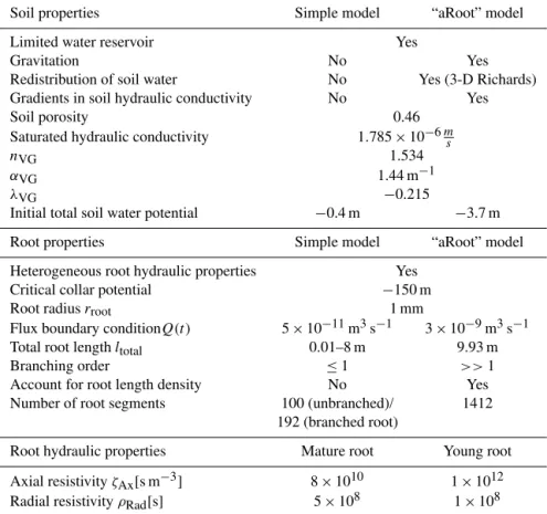
Table 1.Parameters and important features of the simple and the “aRoot” model.
Soil properties Simple model “aRoot” model
Limited water reservoir Yes
Gravitation No Yes
Redistribution of soil water No Yes (3-D Richards) Gradients in soil hydraulic conductivity No Yes
Soil porosity 0.46
Saturated hydraulic conductivity 1.785×10⁻⁶ms
nVG 1.534
αVG 1.44 m−1
λVG −0.215
Initial total soil water potential −0.4 m −3.7 m
Root properties Simple model “aRoot” model
Heterogeneous root hydraulic properties Yes Critical collar potential −150 m
Root radiusrroot 1 mm
Flux boundary conditionQ(t ) 5×10⁻¹¹m3s−1 3×10⁻⁹m3s−1 Total root lengthltotal 0.01–8 m 9.93 m
Branching order ≤1 >>1
Account for root length density No Yes Number of root segments 100 (unbranched)/ 1412
192 (branched root)
Root hydraulic properties Mature root Young root
Axial resistivityζAx[s m−3] 8×10¹⁰ 1×10¹² Radial resistivityρRad[s] 5×10⁸ 1×10⁸
Figure 1.Schematic representation of the root topologies and pa-rameters that were investigated with the simple root water uptake model. Young (lyoung)and mature root length (lmature)are varied independently both in unbranched and branched root structures, re-sulting in varying total length (ltotal)and mature root proportion (pmature). In all heterogeneous cases mature roots constitute the basal part of the root. Within branched roots, total young root length is evenly divided intonparts, which are attached to the central ma-ture root at equal distances. A mixed root strand can equivalently be regarded as a branched root withn=1. Gravity and soil water flow are neglected in the simple model.
average root distance within the complex model. The wa-ter content within each of the soil cylinders is assumed to be spatially constant, but may be different between differ-ent soil segmdiffer-ents. Soil water flow between the soil cylinders
was neglected. All soil cylinders share the same hydraulic properties. The soil water potential ψSoil(i) (m) within each
soil cylinderiis derived from volumetric soil water content θSoil(i) (m3m−3) with a van Genuchten parameterization of the
soilθSoil(i) =f (ψSoil(i)). Parameters are taken from Schneider et
al. (2010) and were originally obtained for a sandy soil (see Table 1 for details). Furthermore, gravitational potential was neglected within the simple model. Thus, the change in soil water status within the soil cylinders is related entirely to root water uptake or release. Simulations are started with initially uniform total soil water potential throughout the entire soil domain (hydrostatic equilibrium).
Water transport within the roots follows an axial pathway, while water uptake (flow from the surrounding soil into the root) occurs along the radial pathway only. Water flow along each pathway is governed by gradients in hydraulic potential and resistances, similar to Ohm’s law. In either direction, the water flow for a given root segmentiis given as
Q(i)Rad=ψ
(i) x −ψSoil(i)
RRad(i)
(1)
Q(i)Ax,in=X
j
ψx(j )−ψx(i)
RAx(j )
Q(i)Ax,out=ψ
(i) x −ψx(k)
RAx(i)
, (3)
whereQ(i)Ax,in,Q(i)Ax,outandQ(i)Rad(m3s−1) are the volumetric
rates of water flow along the axial pathway into root seg-menti, out of root segmenti and along the radial pathway
from the soil into root segmenti.ψx(i),ψx(j ),ψx(k)andψSoil(i)
(m) are the xylem water potentials within the root segment
i, all subsequently connected root segmentsj and the
pre-ceding root segmentk,as well as the bulk soil water
poten-tial within the soil surrounding the root segmenti. Finally, RAx(i)andR(i)Rad(s m−2) are the axial and radial root resistance
within segmenti. These resistances are derived from material
properties and scale with geometric dimensions as follows:
RAx(i)=ζAx(i)·l(i) (4)
RRad(i) = ρ
(i)
Rad
A(i)Surf
= ρ
(i)
Rad
2·π·r(i)·l(i). (5)
The factors ζAx(i) (s m−3) and ρRad(i) (s) are the axial and
ra-dial root hydraulic resistivity of root segmenti. Although the
resistancesRAx(i)andR(i)Raddetermine water flow along
poten-tial gradients in the model, the underlying axial and radial root resistivitiesζAx(i)andρRad(i) define root hydraulic
proper-ties and can be obtained via measurements. Each root seg-ment obtains root hydraulic resistivities corresponding to two discrete hydraulic classes taken from Schneider et al. (2010) (see Table 1). Heterogeneity of root hydraulic properties is introduced in roots by associating these different hydraulic classes with different regions of the root system (see Sect. 2.3 below).
As a consequence of mass conservation and the absence of storage capacities within the root, the water mass balance holds for each segmenti:
Q(i)Ax,in+QRad(i) =Q(i)Ax,out. (6)
By substituting the axial and radial flow rates by Eqs. (1), (2) and (3) for all nroot segments, by denoting Q(Ax0) (m3s−1)
andψx(0)(m) as the unknown total outflow and water
poten-tial at the root collar, and by setting Q(i)Ax,in=0 at the root tips, we obtain n equations for the n+1 unknown xylem water potentials including ψx(0). Closure of this system of
equations is achieved by fixing a boundary condition at the root collar. In our model, this can either be a prescribed (time-dependent) flux rateQ(Ax0)(t )or a constant xylem
wa-ter potential ψx(0). The former represents a given
transpira-tional demand of a plant at a given time; the latter is used to simulate a plant under water stress. At the onset of water
stress transpiration reduces, as collar potential does not fur-ther decrease. All simulations are started with a flux bound-ary condition until collar potential drops to a critical thresh-old (here taken as a typical value of the permanent wilt-ing pointψCrit= −150 m/−1.5 MPa) upon which the
bound-ary condition switches to the potential boundbound-ary condition
ψx(0)=ψCrit= −150 m, thus mimicking “isohydric plants”. After all soil and xylem water potentials have been cal-culated, root water uptake rates can be deduced using Eq. (1) and soil water status is updated using a steady-state approach for a sufficiently short interval of time1t(s)
θSoil;(i) new=θSoil;(i) old−Q
(i)
Rad·1t
VSoil(i)
, (7)
whereVSoil(i) (m3) is the total volume of soil surrounding the
root segment i. The soil water potential decreases
corre-spondingly.
The strongly simplified assumptions within this model al-low for investigation of feedbacks between the distribution of soil water potential and root water uptake, depending on different root hydraulic architectures. In particular, they al-low for understanding the combined role of heterogeneous root hydraulic properties and branching for root water up-take dynamics, which would be hard to detect at a higher level of complexity. In order to test whether the results are reproduced in more realistic conditions, we compare them against the complex root water uptake model, which explic-itly accounts for soil water flow and gravitational potential as described in the next section.
2.2 Root water uptake model for complete root systems We modelled root water uptake in complete root systems of a single plant individual with the three-dimensional root water uptake model “aRoot”, developed by Schneider et al. (2010). We simulate a pot experiment where a complete root sys-tem is embedded in one block of soil with a volume of
2.3 Systematic variation of root hydraulic properties in roots
Both at the single root and at the single-plant scale, the com-plex process of root maturation is simplified by introduc-ing two discrete root hydraulic classes. These two classes possess both different axial and radial resistivities ζAx(i)and ρRad(i), as well as different ratios of radial and axial resistivity ρRad(i)/ζAx(i). Values are taken from Schneider et al. (2010) and
refer to “young” and “mature” roots of a 28-day-old sorghum plant. For reasons of simplicity the root radius is set equal to 1 mm for both young and mature roots. This simplification has little influence on values for root resistances, since de-pendence on root radius is small compared to dede-pendence on root length (see Eqs. 4 and 5).
In order to assess the influence of heterogeneity of root hydraulic properties, the distribution of the two hydraulic classes along the roots is varied systematically. For this, we neglect information about root age or geometry, as we do not focus on reproducing a specific plant. However, we assume that mature roots always constitute the basal parts and young roots the apical parts in all roots. This is achieved differently at the single-root and at the single-plant scale.
Single unbranched and branched roots are created using three parameters: (a) total root length (ltotal), (b) the
propor-tion of young or mature roots (pyoungorpmature)which have
to sum up to one, and (c) the number of root tips (n).
Fig-ure 1 illustrates the construction of single roots used within the simple model. In unbranched single roots the mature root is located in the basal, the young root in the apical part of the root. We modelled unbranched single roots with a to-tal length between 1 and 800 cm, containing between 0 and 100 % of mature roots. Branched single roots are assumed to have two, three, four or six young root branches. All of those branches are distributed evenly along a central mature root strand and have equal lengths, resulting in fishbone-like structures. For branched single roots,ltotalis varied between 5 and 400 cm and pmaturevaries between 10 and 90 %. We are aware that unbranched roots of great length are unreal-istic. However, this artificial set-up allows for assessing the efficiency of root water uptake depending on the branching structure.
At the single-plant scale, the assignment of root hydraulic properties is somewhat different, as root geometry and topol-ogy are given a priori. The root system geometry is obtained with the root generator “RootTyp” by Pagès et al. (2004) and the location of the roots within the soil was kept the same for all simulations (see Fig. 7). The parameters used for “Root-Typ” are taken from Schneider et al. (2010) and correspond to a 28-day-old sorghum plant. The resulting total root length was ltotal=9.93 m. In order to investigate the influence of
heterogeneous hydraulic properties on spatiotemporal root water uptake and its efficiency, we varied the proportions of young and mature roots in steps of 20 % between 0 and
100 % on this geometry as follows: first, starting at the outer ends of the root system, all tip segments were classified as young roots. Afterwards, this assignment was iterated with the immediately preceding segments. The assignment was suspended at branching points until all branches associated with this point were classified entirely (as young roots). If the desired amount of young roots is achieved, the remaining segments are classified as mature roots. This ensures that ma-ture roots are never preceded by young roots and they there-fore constitute the basal and apical root part, respectively. Please note that this manipulation of the root properties was not performed with the intention of to re-produce a natural plant, but to discover shortcomings in root parameterization. 2.4 Measuring the efficiency of root water uptake In order to compare the efficiency of the root water uptake process between different root topologies and degrees of het-erogeneity of root hydraulic properties, we define two in-dices: “water yield” and “effort”.
Water yield v(t ) (m3m−1) assesses how much water VH2Ounstressed (m3) could be taken up per unit root length under
unstressed conditions within a given time:
v(t )=V unstressed H2O (t )
lTotal(t ) =
t
R
τ=0
χ (τ )·Q(τ )dτ
lTotal(t ) , (8)
whereQ(τ )(m3s−1) is the transpirational demand at timeτ
(s) andχ (τ )is used to indicate water stress at timeτ by zero
and one otherwise. Thus, root water uptake under stressed conditions does not contribute to water yield. As stated above, we assume that water stress occurs when xylem water potential at the collarψx(0)(m) drops belowψCrit= −150 m (−1.5 MPa). We normalize by total root length to obtain un-stressed transpiration per invested metre root length, in order to reflect on the increased soil water reservoir available to longer roots.
Expression (8) simplifies for certain conditions. For all simulations presented in this paper, we will be assuming a time-constant transpiration rateQ(t )=Qand a drying
sce-nario. This ensures the existence of a unique pointt˜(s) in time at which water stress occurs. In that case and assuming the absence of storage capacities within the root system, wa-ter yield is directly proportional both to the transpirational demandQand the time at which water stress occurs. If root
growth is furthermore neglected (ltotal= const.), water yield
v(t )can be calculated as
v(t )=
( Q·t
lTotal t <t˜ ˜
v=lQ·˜t
Total t≥ ˜t .
(9)
simply as v˜. The lowercase “v” indicates that water yield
is a normalized volume of water uptake. Assuming a time-constant transpiration rateQ= const. is a strong
simplifica-tion made here for matters of simplicity. However, it does not limit the application of the index to transient conditions.
Effortw(t )(J m−3) is a time-dependent quantity that
mea-sures the average workW (t )(J) necessary to take up a unit of
waterVH2O(t ), and is evaluated over a given interval of time.
Following thermodynamic principles (see Appendix A),w(t )
can be derived from the transpirational demandQ(τ )and the
collar potentialψx(0)(τ ). It takes the following form:
w(t )= W (t )
VH2O(t )=
t
R
τ=0
Q(τ )·ψx(0)(τ )dτ t
R
τ=0
Q(τ )dτ
. (10)
Effort uses the temporal evolution of xylem water potential at the root collarψx(0)to estimate the efficiency of root
wa-ter uptake. According to Eq. (10), it can be inwa-terpreted as a flow-weighted average collar potential. In accordance with
ψx(0) effort has units of a negative hydraulic head (m water
column). Please note that the pressure of 1 MPa can alterna-tively be stated as a hydraulic head of 101,97 m water col-umn, but also has the physical meaning (and units) of an energy density of 106J m−3. The effortw(t )therefore also
has units of a specific energy and we refer to the absolute values of w when saying “effort is minimized”. Under the
conditions stated above (time constant transpiration rateQ, a
drying scenario with unique occurrence time of water stress ˜
t ), Eq. (10) simplifies fort≤ ˜t and effort can be described
with another interesting meaning:
w(t )= Rt
τ=0Q(τ )·ψ (0) x (τ )dτ
Rt
τ=0Q(τ )dτ
=Q· Rt
τ=0ψ (0) x (τ )dτ
Q·t
= ¯ψx(0)(t ) (11)
in which ψ¯0
x(t )(m) is the time-average collar potential
be-tween timesτ=0 andτ=t. In contrast to water yield, effort
still changes after the onset of water stress. But as this con-tribution is very small (see App. A) we will approximate the effort under our specific model conditions withw˜ =w(t )˜ =
¯
ψx0(t )˜. As for water yield, the lowercase “w” indicates that
effort corresponds to a specific (normalized) energy. Assum-ing a time-constant transpirational demand Q= const. is a
strong assumption which is made here for reasons of simplic-ity, but does not limit the application of the index to transient conditions.
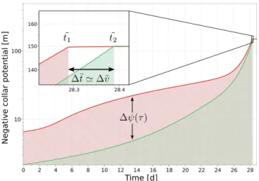
Figure 2 illustrates how water yield and effort can be used to compare the efficiency of root water uptake for one branched (green) and one unbranched (red) single root, both sharing the same total length. Under the above-mentioned conditions, they can be deduced from the temporal evolution of xylem water potential at the root collar. As the total root
Figure 2.Evolution of collar xylem water potential over the course of time for two exemplary chosen single roots of equal total length (0.8 m): an unbranched homogeneous young root (red) and a branched root with six tips (green). Water yield measures the to-tal amount of water that could be extracted before reaching critical xylem water potential. Effort is given by the area below the graph, divided by the respective occurrence times of water stress. Although water yield is very similar between the two root structures in this case, effort is substantially different.
length is the same, water yieldv˜ is directly proportional to the time at which the plant enters water stresst˜(see Eq. 10). In this case, differences in the respective values oft˜andv˜ are very small. Effortw˜ corresponds to the area below the two curves, divided by the respective values oft˜. The green area is much smaller than the red area, which indicates that on average a less negative collar potential and consequently less energy was needed for maintaining root water uptake in the branched root. As all other parameters were equal, this indicates an overall lower resistance to root water uptake ex-perienced by the branched compared to the unbranched root. In this particular case, the differences are induced by branching (see Sect. 3). Water yield is related to the total amount of water that could be extracted under unstressed conditions (unstressed transpiration), but is additionally ref-erenced to total root length. Unstressed transpiration was used before by other researchers to evaluate root parameter-izations (Schneider et al., 2010; Javaux et al., 2008). On the other hand, effort relates to the temporal evolution of xylem water potential at the root collar and the average work nec-essary for root water uptake. It includes information on the total resistance to root water uptake a root system has to over-come and also depends on the soil water retention. As far as we are aware, both indices are novel ways of measuring plant performance, and carry physiological as well as hydrological meaning.
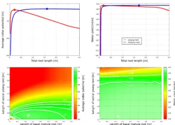
Figure 3.Effortw˜ (left) and water yieldv˜(right) in unbranched sin-gle roots, depending on the proportion of young and mature roots. Data was obtained with the simple model. Shown are effort and wa-ter yield for (top) unbranched homogeneous young (red) and mature (blue) roots over total root length and (bottom) for heterogeneous roots. Optimal values are indicated with circles.
for embolism across climates, plants should apply strategies to avoid very negative xylem water potentials. As lower effort is tantamount for lower average xylem water potentials, it recommends itself as a tool for distinguishing efficient from less efficient parameterizations.
3 Results
We first present results obtained from the simple model sepa-rately for single unbranched and branched roots and next the results obtained with the more encompassing aRoot model for entire root systems.
3.1 Optimal effort and water yield in unbranched single roots
Figure 3 shows effort (top left) and water yield (top right) in unbranched single roots with homogenous root hydraulic properties and increasing length. For both mature and young roots, optimal root lengths emerge. This implies that the av-erage xylem potential (effort) assumes a minimum and the average uptake per root length a maximum at a given root length. Both indices propose similar optimal root lengths (Table 2), but different ones for young and mature roots: young roots have to be short in order to achieve optimal ef-fort and water yield, whereas mature roots have to be long. Interestingly, the actual values at the respective optima are not much different – it is (almost) as efficient to be a short young root as it is to be a long mature root. Water yield is by far the lesser sensitive of the both measures with regard to changes in root length. Also, mature roots exhibit less
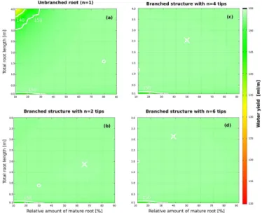
pro-Figure 4.Effortw˜ depending on topology and composition of sin-gle roots, obtained with the simple model. Results are shown for (a)unbranched roots and branched roots (fishbone structures) with (b)two,(c)four and(d)six tips. Root composition is given by to-tal root length (yaxis) and the proportion of mature roots (xaxis). Colours are the same as in Fig. 3 (bottom left). Optimal values of effort are denoted by white circles. The crosses in(b–d)indicate effort for a root that is the same as the optimal unbranched hetero-geneous root from(a)except for containing one, three and five more equal young root tips, respectively.
nounced differential changes in effort and water yield than young roots when changing root length.
Results for heterogeneous unbranched roots are shown at the bottom of Fig. 3. All heterogeneous single roots consist of basal mature and apical young roots. Heterogeneity affects the efficiency at the respective optimal lengths differently: optimal heterogeneous roots have decreased their effort by 15 %, but increased their water yield only slightly by 1 %. Moreover, for the optimal mixed root strand, the optimal to-tal root lengths are shorter than expected, in that the optimal mixed root strand is not a composition of an optimal mature root strand and an optimal young root strand, but altogether shorter (Table 2). In composed roots some of the water is taken up by the basal mature root part and less water has to be transported through the apical young roots. Therefore drops in xylem potential are smaller, axial limitation is less severe and the hydraulically active young root region is extended in composed roots. For this reason, in optimal composed roots, young roots are longer and mature roots are shorter compared to their homogenous peers. This leads to overall shorter com-posite unbranched single roots.
3.2 Optimal effort and water yield in branched single roots
Table 2.Optimal compositions of single roots referring to effort (top) and water yield (bottom). Results are obtained with the simple model for different root topologies.
lyoung
Structure ltotal lmature lyoung per branch w˜ Young root strand 0.20 m – 0.20 m/100 % 0.20 m −18.0 m Mature root strand 1.60 m 1.60 m/100 % – – −15.3 m Mixed root strand 1.50 m 1.20 m/80 % 0.30 m/20 % 0.30 m −15.1 m Branched root, 2 tips 1.30 m 0.65 m/50 % 0.65 m/50 % 0.33 m −14.4 m Branched root, 3 tips 0.90 m 0.09 m/10 % 0.81 m/90 % 0.27 m −13.5 m Branched root, 4 tips 1.20 m 0.12 m/10 % 1.08 m/90 % 0.27 m −12.8 m Branched root, 6 tips 1.60 m 0.16 m/10 % 1.44 m/90 % 0.24 m −12.3 m
lyoung
Structure ltotal lmature lyoung per branch v˜ Young root strand 0.15 m – 0.15 m/100 % 0.15 m 153.07 cm−3m−1 Mature root strand 1.80 m 1.80 m/100 % – – 153.21 cm−3m−1 Mixed root strand 1.60 m 1.28 m/80 % 0.32 m/20 % 0.32 m 153.21 cm−3m−1 Branched root, 2 tips 0.90 m 0.27 m/30 % 0.63 m/70 % 0.32 m 153.24 cm−3m−1 Branched root, 3 tips 0.90 m 0.18 m/20 % 0.72 m/80 % 0.24 m 153.28 cm−3m−1 Branched root, 4 tips 1.20 m 0.12 m/10 % 1.08 m/90 % 0.27 m 153.30 cm−3m−1 Branched root, 6 tips 2.00 m 0.20 m/10 % 1.80 m/90 % 0.30 m 153.32 cm−3m−1
optimal combinations are given in Table 2). The root com-position is now given by the total root length of the respec-tive root (yaxis) and the proportion of mature roots (xaxis).
Colours are the same as in Fig. 3 (bottom left). While the proportion of mature roots in optimally branched roots de-creases disproportionately, the total length of all young roots increases almost proportionally to the number of tipsn
(Ta-ble 2). When adding new tips, individual young root branches shorten only a little, allowing for the total root length to expand while also decreasing effort. In this way, branching favours soil exploration, without compromising efficiency. Notably, the effort surface becomes flatter, and hence the do-main of nearly efficient hydraulic parameterizations expands with the number of tips.
Similar results are obtained for water yield but results are far less sensitive (Fig. 5). For all branched roots, water yield is nearly constant (little sensitive) within the domain of mod-elled root compositions and increases only very little com-pared to the optimal unbranched single root (see Table 2).
3.3 Water uptake dynamics and redistribution patterns in single roots
The proportions of root hydraulic properties within a branched or unbranched single root do not only affect the efficiency of root water uptake, but also its location and dy-namics. This may even be the case, if the efficiency is similar between parameterizations. Figure 6 shows root water up-take rates along three exemplarily chosen unbranched roots of equal length (ltotal=0.42 cm) and similar water yield and
Figure 6.Velocity of radial inflow (uptake velocity) at the root sur-face along three unbranched single roots with equal length (ltotal= 0.42 m) but different composition. Values are obtained with the sim-ple model for roots containing young roots only (red), mature roots only (blue) or an optimal mixture with respect to water yield (green; lmature=0.14 m,lyoung=0.28 m). Results are depicted for(a) ini-tial stage (hydrostatic equilibrium), (b)4 days and (c)8 days of simulation time.
effort. They are a young (red), mature (green) and optimally composed mix of apical young and basal mature root (blue). At the initial stage, the young root shows an exponential decrease in root water uptake rate towards the tip, which is at this time hydraulically isolated. In contrast, root wa-ter uptake is distributed almost equally along the mature root strand. The initial uptake pattern of the heterogeneous root is a combination: an almost homogeneous uptake rate in the basal mature root part is followed by an increased rate of root water uptake in the young root part, which decays exponen-tially. After some time (4 days in the model), a moving up-take front (MUF) has developed both in the pure young and in the mixed root strand, reaching the root tip after 8 days. Additionally, in the heterogeneous root, water uptake in the basal mature root part increases with time. In contrast, in the pure mature root, the water uptake profile is static and does not change much over the course of the simulation. Although the occurrence of moving uptake fronts is accentuated by the neglect of soil water flow and gravity within the simple root water uptake model, qualitatively the same results are ob-tained within the complex “aRoot” model, in which soil wa-ter flow and gravity are explicitly considered (see Sect. 3.5 and Fig. 7).
3.4 Effort and water yield in entire root systems In order to quantify what influence the above-mentioned small-scale processes have at the scale of an individual plant, and taking soil water flow and gravitation into account, we used the detailed three-dimensional root water uptake model
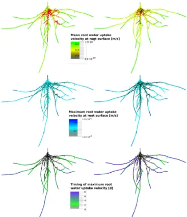
Figure 7.Root water uptake dynamics in a fixed root geometry with two different hydraulic parameterizations. Results were obtained with the “aRoot” model for one root system containing young roots only (left, least efficient) and a mixture of 40 % of basal mature and 60 % of apical young roots (right, most efficient). (Top) Time-averaged root water uptake rate along the root system. Regions with negative net uptake (hydraulic lift or bleeding) are depicted in red, independent of the actual amount of water released. (Centre) Mag-nitude and (bottom) timing of maximum uptake velocity along the root system. Please note the log-scale of the colour bar in the top and centre panel.
“aRoot”. We calculated effort and water yield along with spa-tiotemporal root water uptake for one exemplary root sys-tem geometry, which was kept the same for all simulations (see Fig. 7 for geometry). Only the proportions of young and mature roots were systematically varied in steps of 20 % be-tween 0 and 100 % (see Sect. 2.3).
less efficient, because the potential of young roots was not fully explored (Sect. 3.2).
In order to preclude that our results are subject to an ar-tifact of the evaluation time (i.e. the different time of first occurrence of water stress at which effort is calculated), we also evaluated effort 5 days after the start of the simulation, and confirmed that the ranking of the root systems did not change (Table 3). Additionally, we repeated our analysis with a transient (sinusoidal) transpirational demand and qualita-tively obtained the same results (see Supplement).
3.5 Water uptake dynamics and redistribution patterns in entire root systems
Figure 7 compares the spatial distribution of root water up-take characteristics in a homogenous (least efficient) and het-erogenous (most efficient) root system. Mean root water up-take rates upup-take rates (top) vary much less in the homoge-neous compared to the heterogehomoge-neous root system (spanning 1 order of magnitude compared to 3 orders of magnitude). Also, within all heterogeneous root systems, water uptake of mature roots is always smaller than the mature root propor-tion (Fig. 8, left). This indicates the separapropor-tion of root func-tion in the heterogeneous root system between uptake roots and transport roots, and is in agreement with the earlier ob-servations in the simple model. Apical young roots have a higher mean uptake rate than inner young roots in both hy-draulic parameterizations, which is due to higher root density in the central parts of the root system.
The lower part of Fig. 7 shows the magnitude (centre) and timing (bottom) of the maximum uptake at each location of the root system. This allows for the tracking of moving up-take fronts. The timing of the maximum shows how upup-take moves evenly away from the collar in the young root system as expected from the simple model (see Fig. 6). In hetero-geneous root systems the uptake pattern is more complex. Maximum uptake rates occur in the young roots, irrespective of their actual position within the root system (see Sect. 2.4 for the distribution of root hydraulic properties). The timing of the maximum uptake shows that uptake fronts move not only outwards but also inwards (see the blue roots in the cen-tre of the root system, Fig. 7, bottom right). Inner mature roots are activated late and only if the surrounding soil was not previously dried out by young roots. Together with dis-tant young roots, mature roots contribute the majority to total water uptake after 8 days (see Figs. 7 and 8). This redistribu-tion pattern corresponds to the one observed with the simple model in heterogeneous single roots (Sect. 3.3 and Fig. 6). In the simple model, root water uptake was redistributed in two ways: “forward” along young roots towards the root tips by moving uptake fronts; and “backward” away from distal young roots to inner mature roots. In the complex “aRoot” model, which considers root length density and soil water redistribution, a third redistribution pattern is added: redistri-bution between different root branches. Root water uptake is
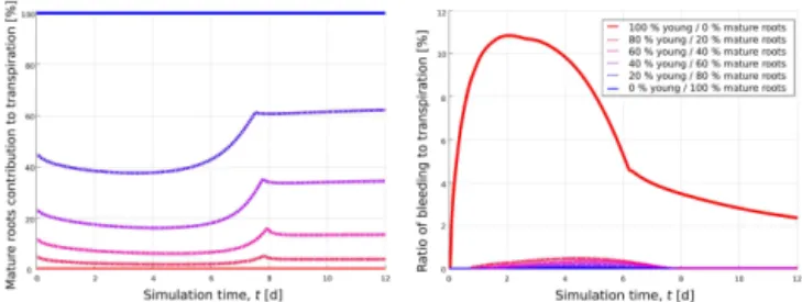
Figure 8.Evolution of mature root contribution to overall transpira-tion (left) and the ratio of bleeding (right) over time in the fixed root geometry for the six different hydraulic parameterizations. Results are obtained with the “aRoot” model for fractions of apical young roots between 0 and 100 %. Homogeneous root systems are de-picted in solid lines; heterogeneous root systems are dede-picted with dashed lines.
distributed away from (inner) branches of young and mature roots, as they fall dry in the course of soil drying, and is redis-tributed towards roots in wetter soils. Altogether, this leads to higher efficiency in heterogeneous root systems compared to homogeneous root systems (see Table 3), which is likely due to a more efficient compensation for local water stress and enhanced soil exploration.
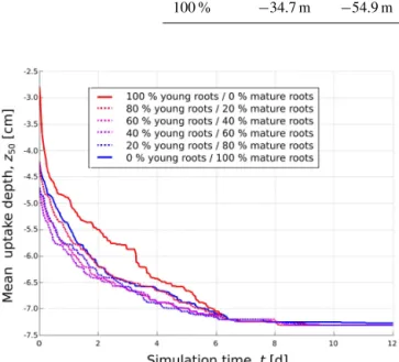
Uptake depth in root systems with mature roots was deeper compared to homogenous root systems for much of the sim-ulation time. Figure 9 shows temporal evolution of the depth
z50 (m) above which half of the root water uptake occurred. Over the course of time,z50 moves downwards in all hy-draulic parameterizations and equilibrates at the onset of wa-ter stress, with the homogeneous young root system being most dynamical, and most shallow at the same time.
Hydraulic lift occurred in all root parameterizations. How-ever, the domain of hydraulic lift is noticeably larger in the homogenous young root system compared to all other hy-draulic parameterizations. Both the total length of bleeding roots and the absolute amount of water released decrease along with young root proportion, being smallest in the ho-mogeneous mature root system (see also Fig. 8, right). The by far highest values of hydraulic lift are modelled for the the homogeneous young root system (up to 10 % of total root water uptake). It must be stated that bleeding usually occurs at night and may hence not be well captured with the time-constant flux boundary condition used here. However, simulations with a sinusoidal day/night cycle of transpiration showed qualitatively the same results.
4 Discussion
Table 3.Initial collar potentialψx0(t=0), effort after 5 days of simulation timew(t=5d), effort at the onset of water stressw˜, water yield at the onset of water stressv˜ and mean uptake depthz50 for the fixed root geometry with a total length ofltotal=9.93 m, depending on hydraulic parameterization. Data were obtained with the “aRoot” model for roots containing between 0 and 100 % of mature roots.
pmature ψx(0)(t=0) w(t=5d) w˜ v˜ z50 0 % −67.0 m −98.4 m −105.2 m 162.1 cm3m−1 −6.55 cm 20 % −15.7 m −30.0 m −44.1 m 205.4 cm3m−1 −6.78 cm 40 % −16.8 m −28.9 m −42.7 m 207.5 cm3m−1 −6.87 cm 60 % −19.1 m −32.1 m −46.4 m 203.4 cm3m−1 −6.90 cm 80 % −23.6 m −39.4 m −54.2 m 196.4 cm3m−1 −6.86 cm 100 % −34.7 m −54.9 m −77.8 m 174.2 cm3m−1 −6.74 cm
Figure 9.Temporal evolution of mean uptake depthz50in the fixed root geometry for the six different hydraulic parameterizations. Re-sults are obtained with the “aRoot” model for proportions of young roots between 0 and 100 %. Homogeneous root systems are de-picted in solid lines; heterogeneous root systems are dede-picted with dashed lines.
to have homogenous hydraulic properties and to be in hydro-static equilibrium at the initial stage. Second, soil water re-distribution and gravity were only considered in the complex “aRoot” model. This rather strong simplification in the sim-ple model facilitates understanding the process of root water uptake redistribution. Qualitatively similar effects were ob-tained with the complex model, which explicitly accounts for soil water flow and gravitation. Third, the presented results were obtained assuming an idealized drying scenario with a time constant flux boundary condition. We do this mainly to facilitate comparison of different hydraulic parameteriza-tions. The general definitions of water yield and effort given in Eqs. (8) and (10) are applicable under arbitrary bound-ary conditions. In order to validate that our results do not depend on specific assumptions, the same analysis was also performed with a sinusoidal transpiration rate in which re-sults remained qualitatively the same (see Supplement). In particular, the ranking of the six hydraulic parameterizations
remained the same with regard to temporal evolution of col-lar potential, water yield and effort, as well as the amount of simulated hydraulic lift (bleeding).
We combine two approaches from Schneider et al. (2010) and Doussan et al. (2006) to generate heterogeneity of root hydraulic properties in roots: first we use two classes of roots with both distinct radial and axial resistivities (young and mature roots). Second, we systematically change the degree of heterogeneity within the respective root by altering the proportions of these two root classes a priori, and by sub-sequently neglecting both root growth and maturation dur-ing the modelldur-ing period. Although roots are reported to alter their hydraulic properties according to parameters like topol-ogy, diameter and age (Frensch and Steudle, 1989; Steudle and Peterson, 1998; Doussan et al., 2006), we assume that this will not affect our results at the model timescale. Fur-thermore, these idealizations allow us to neglect processes (which themselves demand detailed but mainly unknown in-formation and parameters) and facilitate both the description of root water uptake mechanisms and the detection of ax-ial and radax-ial limitation. Generally, considering root matura-tion by incremental changes of hydraulic properties within each class as in Doussan et al. (2006) or the further addi-tion of classes as in Schneider et al. (2010) is possible and would further enhance the complex redistribution patterns described in this paper. We suppose that efficient strategies of root growth and maturation also change with climate, in particular with drying and rewetting of the soil by precipita-tion, which we have not considered in this paper. We expect that the sensitivity of model results to parameterization will be more pronounced under more realistic situations, in larger root networks and in plant communities (Kalbacher et al., 2011).
Taken together, we believe our model idealizations serve the purpose of discovering drivers that shape root water up-take patterns, which are difficult to discover in more compre-hensive simulations; and to capture the essential features to yield process insight.
to carbon uptake, and the fact that it is relatively easy to mea-sure in experiments, transpiration appears in modelling stud-ies of root water uptake (Doussan et al., 2006; Javaux et al., 2008; Schneider et al., 2010). In contrast, temporal evolution of xylem water potential at the root collar is usually not dis-cussed in detail, although it is of importance for the plant function. Large negative xylem potentials may lead to cavi-tation, i.e. the disconnection of the water column within the xylem conduits and interruptions of water transport (Tyree and Sperry, 1989; Pockman and Sperry, 2000). As cavita-tion reduces hydraulic conductivity in root xylem, effort may be related to a plant’s ability to exploit soil water and to sustain droughts (McDowell et al., 2008). We observe that water yield and effort deliver similar results on the numeric value of optimal root length for a given parameterization, but show different sensitivity, with effort being more sensitive to changes in parameterization than water yield. Thus effort suggests itself as an efficiency criterion, which may even be more meaningful to plants than water yield. Together with simulators for root architecture (Pagès et al., 2004; Leitner et al., 2010), and given knowledge of critical xylem pressures, effort may be a helpful index for identifying efficient root hydraulic parameterizations of given species.
For our indices we used time-integrated measures of effi-ciency in order to account for the activation of initially hy-draulically isolated regions of the root system by moving up-take fronts. Recently, other indices have been proposed to capture both the root hydraulic conductivity of entire root systems (KRS)and effective soil water potentials (Couvreur
et al., 2012). While moving uptake fronts help soil explo-ration, in parallel the xylem potential has to be decreased substantially. The time-averaged xylem potential therefore gives an integrated index encompassing both the overall root hydraulic conductivity (KRS)as well as the capacity to
ac-tivate uptake length further. Beyond the optimum, it is hy-draulically more efficient to invest in a new root than pro-long an existing one. We defined this as the separating point between radial and axial limitation, as opposed to hydraulic isolation (Zwieniecki et al., 2003; North and Peterson, 2005). Neither of our indices balances the hydraulic efficiency with carbon cost, although water yield carries some information on biomass investment, as it gives the water uptake per root length. The next steps would be to consider the carbon invest-ment in root maturation and turnover with insights from our model or coupling it with models of stomata opening (Tuzet et al., 2003) to assess carbon gain.
The compensation of local water stress in young roots, which extends hydraulically active root length by moving uptake fronts, agrees with other models and observations (Roose and Fowler, 2004; Garrigues et al., 2006). Never-theless, young root strands suffer from axial limitation when they are too long. We observed that unbranched young roots possess optimal lengths in the range of some centimetres, whereas optimal lengths of unbranched mature roots may be in the range of metres. All optimal heterogeneous hydraulic
parameterizations were more efficient than the correspond-ing homogenous ones, which is intuitive and consistent with observations showing that roots differentiate with maturation (Frensch and Steudle, 1989; Doussan et al., 2006). Thus, root maturation is meaningful from a hydraulic point of view, as it keeps young roots short. Furthermore, overall root water up-take is much more efficient, when the active length of young roots is increased by branching, since this decreases axial limitation.
For root systems, which divide their functioning into root water uptake and transport, active young root length in-creases. Mature roots with higher axial conductivity act as a transport system for uptake delivered from many individ-ual short young roots with high radial conductivity. In other words, transmitting the collar xylem potential effectively to the young root branches is preferably done by mature trans-port roots in central parts of the heterogeneous root system. This rather intuitive result needs to be considered when pa-rameterizing models for hydrological applications as it also impacts root water uptake dynamics.
In the more realistic and efficient heterogeneous root sys-tems, spatiotemporal uptake behaviour becomes complex. As long as the soil is moist, water uptake is achieved through young roots with uptake starting near the branching points, as was already pointed out by Roose and Fowler (2004), and agrees with experimental results from Zarebanadkouki et al. (2013) on lupines. As the soil around the branching points dries out, water uptake is redistributed to the apical ends of the central young roots by moving uptake fronts. Particularly in the heterogeneous root systems, the temporal evolution of water uptake is the result of several interacting re-distribution patterns, which do not only move vertically, but also hori-zontally, and not only from top to bottom, but also from the bottom up, depending as well on the density of young roots. By this, plants with heterogeneous root hydraulic properties have more possibilities to compensate for local water stress in distinct regions of the root system, which likely leads to in-creased water yield at dein-creased effort. Surprisingly, chang-ing the proportion of mature roots between 20 and 60 % re-sulted in similar, nearly optimal values of both water yield and effort, suggesting that a precise consideration of hetero-geneity may not be necessary.
contrast, our results show the highest amount of bleeding in the most inefficient root hydraulic parameterization, namely in the homogeneous young root system. This result remained unaltered when a sinusoidal transpirational demand was used instead of a fixed flux boundary condition. This indicates that bleeding in this case did not act to improve the overall water status of the plant. Thus although hydraulic redistribution is frequently observed in the real world (Neumann and Cardon, 2012), its occurrence in models does not necessarily imply efficient parameterization.
5 Conclusions
In this modelling study we show that root hydraulic proper-ties, in particular the ratio of root radial and axial resistiv-ity, determine optimal root length for single roots in a drying scenario. We investigate this with two different indices intro-duced to compare the efficiency of root water uptake: water yield and effort. Water yield measures the amount of root wa-ter uptake extracted from the soil before a plant enwa-ters wawa-ter stress; effort indicates the xylem water potential (average en-ergy) necessary for this root water uptake under unstressed conditions. Both are suitable to detect efficient lengths of young and mature roots, with effort being more sensitive than water yield. Optimal lengths of unbranched young roots are some centimetres, compared to several metres for ma-ture roots. However, the efficiency of simulated root water uptake increases, when more young root length can be ac-tivated. This is achieved in branched roots with heteroge-neous root hydraulic properties, which allow for a division of function between water uptake and transport. This finding is supported by simulations in a complex three-dimensional root system, where mature roots contribute disproportion-ately less to overall root water uptake compared to young roots, suggesting that they act as transport roots.
Appendix A: The functional form of effort and its depen-dence on boundary conditions
Any water potentialψw(m or 9810 J m−3) describes the spe-cific Gibbs free energy of water (Edlefsen and Anderson, 1948, article 62), comparable to the chemical potential. Dif-ferential changes in Gibbs free energy 1G(J) in a system
under consideration over a short period of time 1t (s) are
therefore
1G=ψw·1Vw, (A1)
where1Vw(m3) refers to the change of water volume in the system. When the system is closed and the change of energy is caused by a water flowQw(m3s−1) over the boundary of the system, the above equation becomes
1G=ψw·Qw·1t. (A2)
Applying these equations to the coupled plant–root system in a closed container, where the only water flow out of the system is by root water uptake, we can therefore state that the change in Gibbs free energy of the system from a starting pointt0(s) up to a timet (s) under consideration is
G(t )=
t
Z
τ=t0
ψC(τ )·Q(τ )dτ , (A3)
whereψC(τ )(m) refers to the water potential at the root
col-lar at timeτ (s).
As the change of Gibbs free energy to go from state A to state B of a closed system equals the mechanical work to go from A to B (neglecting the work of expansion, Edlef-sen and Anderson, 1948, article 21, 62), G(t )is equivalent
to the work required for root water uptake. We can define a normalized measure,w(t )(J m−3), which evaluates average
work required per unit of water transpired betweent0andt:
w(t )= G(t )
t
R
τ=t0
Q(τ )dτ
=
t
R
τ=t0
ψC(τ )·Q(τ )dτ
t
R
τ=t0
Q(τ )dτ
. (A4)
This means that under arbitrary boundary conditions, effort can be understood as a flow-weighted average xylem water potential at the root collar.
Under a drying scenario, root water uptake causes soil wa-ter potential to decrease monotonically. Thus, at a unique timet˜(s) plant water stress occurs. Effort at timet˜will in this case be denoted byw˜=w(t )˜. Under a time constant transpi-ration rateQ(τ )=Q, effortw˜=w(t )˜ can be calculated as a
temporal average xylem water potential at the root collar:
˜
w=w(t )˜ = ˜
t
R
τ=0
Q(τ )·ψC(τ )dτ
˜ t R τ=0 Q(τ )dτ = Q· ˜ t R τ=0
ψC(τ )
Q· ˜t
= ˜
t
R
τ=0
ψC(τ )dτ
˜
t = ¯ψC(t ).˜ (A5)
In contrast to water yield, effort increases under water stress. However, this increase is small, as will be shown in the fol-lowing.
In order to calculate effort at a timet >t˜, we use the gen-eral definition of effort and split the integrals in the enumer-ator and and denominenumer-ator at the occurence of water stresst˜
w(t )=
t
R
τ=0
Q(τ )·ψC(τ )dτ
t R τ=0 Q(τ )dτ = ˜ t R τ=0
Q(τ )·ψC(τ )dτ+
t
R
τ=˜t
Q(τ )·ψC(τ )dτ
˜
t
R
τ=0
Q(τ )dτ+
t
R
τ=˜t
Q(τ )dτ
. (A6)
We can now insert the flux boundary conditionQ(τ )=Qfor
timesτ =0. . .t˜and the potential boundary conditionψ (τ )=
ψcritfor timesτ = ˜t . . .t. We obtain
w(t )= ˜
t
R
τ=0
Q(τ )·ψC(τ )dτ+
t
R
τ=˜t
Q(τ )·ψC(τ )dτ
˜
t
R
τ=0
Q(τ )dτ+
t
R
τ=˜t
Q(τ )dτ = Q· ˜ t R τ=0
ψC(τ )dτ+ψcrit·
t
R
τ=˜t
Q(τ )dτ
Q· ˜t+
t
R
τ=˜t
Q(τ )dτ
. (A7)
If we transform the integrals in the stress periods by replac-ingτ = ˜t . . .tbyτ=0...1t (1t=t− ˜tis the time since the
occurrence of water stress), effort can be expressed as
w(t )=w(t˜+1t )
= Q· ˜ t R τ=0
ψC(τ )dτ+ψcrit· 1t
R
τ=0
Q(t˜+τ )dτ
Q· ˜t+
1t
R
τ=0
Q(t˜+τ )dτ
By defining EU :=Q·
˜
t
R
τ=0
ψC(τ )dτ =const.,VU=Q· ˜t= const., and Vs(1t )=
1t
R
τ=0
Q(t˜+τ )dτ, effort can be
ex-pressed as
w(t )=w(t˜+1t )=EU+ψcrit·VS(1t )
VU+VS(1t ) =w(Vs(1t )). (A9) EU (J) is the (time-independent) energy that was necessary to take up water under unstressed conditions, it is also the enumerator ofw˜;VU(m3) is the (time-independent) amount of water that was extracted before the onset of water stress, it also is the denominator ofw˜; andVs (m3) is the amount
of water that was extracted after the onset of water stress.Vs
depends on the duration1t of water stress.
Using a first-order Taylor approximation of w around t˜ yields
w(t )=w(t˜+1t )= ˜w+(ψcrit− ˜w)·Vs(1t )
Vu . (A10)
For1t=0 (t= ˜t, the onset of water stress) this
approxima-tion gives the correct valuew˜ of effort. For 1t >0, effort
increases linearly with the amount of waterVs extracted
un-der water stress. But as root water uptake rates of stressed plants decrease quickly in a drying soil, effort increases very slowly with time.
Acknowledgements. Acknowledgements. M. Bechmann was
funded by the Jena School for Microbial Communication (JSMC). A. Hildebrandt was supported partly by AquaDiv@Jena, a project funded by the initiative “ProExzellenz” of the German Federal state of Thuringia. We thank Peer Joachim Koch (Max-Planck-Institute for Biogeochemistry, Jena, Germany) and Thomas Kalbacher (Helmholtz Centre for Environmental Research, Leipzig, Germany) for their support with the hard- and software. We thank the editor Nadia Ursino for handling the discussion process as well as four anonymous reviewers and Axel Kleidon for their insightful comments and in depth discussion of the manuscript.
References
Angeles, G., Bond, B., Boyer, J. S., Brodribb, T., Brooks, J. R., Burns, M. J., Cavender-Bares, J., Clearwater, M., Cochard, H., Comstock, J., Davis, S. D., Domec, J.-C., Donovan, L., Ewers, F., Gartner, B., Hacke, U., Hinckley, T., Holbrook, N. M., Jones, H. G., Kavanagh, K., Law, B., López-Portillo, J., Lovisolo, C., Mar-tin, T., Martínez-Vilalta, J., Mayr, S., Meinzer, F. C., Melcher, P., Mencuccini, M., Mulkey, S., Nardini, A., Neufeld, H. S., Pas-sioura, J., Pockman, W. T., Pratt, R. B., Rambal, S., Richter, H., Sack, L., Salleo, S., Schubert, A., Schulte, P., Sparks, J. P., Sperry, J., Teskey, R., and Tyree, M. T.: The Cohesion-Tension theory, New Phytologist, 163, 451–452, 2004.
Bauerle, T. L., Richards, J. H., Smart, D. R., and Eissenstat, D. M.: Importance of internal hydraulic redistribution for prolonging the lifespan of roots in dry soil, Plant. Cell Environ., 31, 177–186, 2008.
Blum, A.: Crop responses to drought and the interpretation of adap-tion, Plant Growth Regul., 20, 135–148, 1996.
Brooksbank, K., White, D. A., Veneklaas, E. J., and Carter, J. L.: Hydraulic redistribution in Eucalyptus kochii subsp borealis with variable access to fresh groundwater, Trees-Struct. Funct., 25, 735–744, 2011.
Cai, X., Wang, D., and Laurent, L.: Impact of Climate Change on Crop Yield: A Case Study of Rainfed Corn in Central Illinois, J. Appl. Meteorol. Climatol. 48, 1868–1881, 2009.
Caldwell, M. M., Dawson, T. E., and Richards, J. H.: Hydraulic lift: Consequences of water efflux from the roots of plants, Oecolo-gia, 113, 151–161, 1998.
Choat, B., Jansen, S., Brodribb, T. J., Cochard, H., Delzon, S., Bhaskar, R., Bucci, S. J., Feild, T. S., Gleason, S. M., Hacke, U. G., Jacobsen, A. L., Lens, F., Maherali, H., Martinez-Vilalta, J., Mayr, S., Mencuccini, M., Mitchell, P. J., Nardini, A., Pitter-mann, J., Pratt, R. B., Sperry, J. S., Westoby, M., Wright, I. J., and Zanne, A. E.: Global convergence in the vulnerability of forests to drought, Nature, 491, 752–755, 2012
Choat, B.: Predicting thresholds of drought-induced mortality in woody plant species, Tree Physiol., 33, 669–671, 2013. Churkina, G. and Running, S. W.: Contrasting Climatic Controls on
the Estimated Productivity of Global Terrestrial Biomes, Ecosys-tems, 1, 206–215, 1998.
Clausnitzer, V. and Hopmans, J. W.: Simultaneous modelling of transient 3-dimensional root growth and soil water flow, Plant. Soil, 164, 299–314, 1994.
Collins, D. B. G. and Bras, R. L.: Plant rooting strategies in water-limited ecosystems, Water Resour. Res., 43, W06407, doi:10.1029/2006WR005541, 2007
Couvreur, V., Vanderborght, J., and Javaux, M.: A simple three-dimensional macroscopic root water uptake model based on the hydraulic architecture approach, Hydrol. Earth Syst. Sci., 16, 2957–2971, doi:10.5194/hess-16-2957-2012, 2012.
Domec, J.-C., King, J. S., Noormets, A., Treasure, E., Gavazzi, M. J., Sun, G., and McNulty, S. G.: Hydraulic redistribution of soil water by roots affects whole-stand evapotranspiration and net ecosystem carbon exchange, New Phytol., 187, 171–183, 2010. Domec, J. C., Scholz, F. G., Bucci, S. J., Meinzer, F. C., Goldstein,
G., and Villalobos-Vega, R.: Diurnal and seasonal variation in root xylem embolism in neotropical savanna woody species: im-pact on stomatal control of plant water status, Plant. Cell Envi-ron., 29, 26–35, 2006.
Doussan, C., Pierret, A., Garrigues, E., and Pagès, L.: Water uptake by plant roots: II – Modelling of water transfer in the soil root-system with explicit account of flow within the root root-system – Comparison with experiments, Plant Soil, 283, 99–117, 2006. Dunbabin, V. M., Postmam, J. A., Schnepf, A., Pagès, L., Javaux,
M., Wu, L., Leitner, D., Chen, Y. L., Rengel, Z., and Diggle, A. J.: Modelling root–soil interactions using three–dimensional mod-els of root growth, architecture and function, Plant. Soil, 372, 1–2, 93–124, 2013.
Edlefsen, N. and Anderson, A.: Thermodynamics of soil moisture, Hilgardia, 15, 31–298, 1943.
El Maayar, M., Price, D. T., and Chen, J. M.: Simulating daily, monthly and annual water balances in a land surface model us-ing alternative root water uptake schemes, Adv. Water Resour., 32, 1444–1459, 2009.
Feddes, R. A., Kowalik, P. J., and Zaradny, H.: Simulation of Field Water Use and Crop Yield, John Wiley & Sons, 188 pp., 1978. Feddes, R. A., Hoff, H., Bruen, M., Dawson, T. E., Rosnay, P. d.,
Dirmeyer, P., Jackson, R. B., Kabat, P., Kleidon, A., Lilly, A., and Pitman, A. J.: Modeling Root Water Uptake in Hydrological and Climate Models, Bull. Am. Meteorol. Soc., 82, 2797–2809, 2001.
Frensch, J and Steudle, E.: Axial and Radial Hydraulic Resistance to Roots of Maize (Zea mays L.), Plant Physiol., 91, 719–726, 1989.
Garrigues, E., Doussan, C., and Pierret, A.: Water uptake by plant roots: I – Formation and propagation of a water extraction front in mature root systems as evidenced by 2D light transmission imaging, Plant. Soil, 283, 83–98, 2006.
Heppel, C., Payvandi, S., Zygalakis, K. C., Smethurst, J., Fliege, J., and Roose, T.: Validation of a spatial-temporal soil water move-ment and plant water uptake model, Geotechnique, 64, 526–539, 2014.
Hildebrandt, A. and Eltahir, E. A. B.: Ecohydrology of a seasonal cloud forest in Dhofar: 2. Role of clouds, soil type, and root-ing depth in tree-grass competition, Water Resour. Res., 43, W11411, doi:10.1029/2006WR005262, 2007.
Huszár, T., Mika, J., Lóczy, D., Molnár, K., and Kertész, A.: Climate Change and Soil Moisture: A Case Study, Phys. Chem. Earth A, 24, 905–912, 1998.
Jackson, R. B., Sperry, J. S., and Dawson, T. E.: Root water up-take and transport: using physiological processes in global pre-dictions, Trends Plant Sci., 5, 482–488, 2000.
Javaux, M., Schröder, T., Vanderborght, J., and Vereecken, H.: Use of a Three-Dimensional Detailed Modeling Approach for Pre-dicting Root Water Uptake, Vadose Zone J., 7, 1079–1088, 2008. Kalbacher, T., Schneider, C., Wang, W., Hildebrandt, A., Attinger, S., and Kolditz, O.: Modeling Soil-Coupled Water – Uptake of Multiple Root Systems with Automatic Time Stepping, Vadose Zone J., 10, 727–735, 2011.
Katul, G. G., Oren, R., Manzoni, S., Higgins, C., and Parlange, M. B.: Evapotranspiration: A process driving mass transport and en-ergy exchange in the soil-plant-atmosphere-climate system, Rev. Geophys., 50, RG3002, doi:10.1029/2011RG000366, 2012. Kleidon, A. and Heimann, M.: A method of determining rooting