EUROPEAN ORGANIZATION FOR NUCLEAR RESEARCH (CERN)
CERN-EP-2018-058 2018/06/21
CMS-MUO-16-001
Performance of the CMS muon detector and muon
reconstruction with proton-proton collisions at
√
s
=
13 TeV
The CMS Collaboration
∗Abstract
The CMS muon detector system, muon reconstruction software, and high-level trig-ger underwent significant changes in 2013–2014 in preparation for running at higher LHC collision energy and instantaneous luminosity. The performance of the mod-ified system is studied using proton-proton collision data at center-of-mass energy
√
s = 13 TeV, collected at the LHC in 2015 and 2016. The measured performance parameters, including spatial resolution, efficiency, and timing, are found to meet all design specifications and are well reproduced by simulation. Despite the more chal-lenging running conditions, the modified muon system is found to perform as well as, and in many aspects better than, previously. We dedicate this paper to the memory of Prof. Alberto Benvenuti, whose work was fundamental for the CMS muon detector.
Published in the Journal of Instrumentation as doi:10.1088/1748-0221/13/06/P06015.
c
2018 CERN for the benefit of the CMS Collaboration. CC-BY-4.0 license
∗See Appendix A for the list of collaboration members
1
1
Introduction
The Compact Muon Solenoid (CMS) detector at the CERN LHC is a general purpose device designed primarily to search for signatures of new physics in proton-proton (pp) and heavy ion (proton-ion and ion-ion) collisions. Since many of these signatures include muons, CMS is constructed with subdetectors to identify muons, trigger the CMS readout upon their detec-tion, and measure their momentum and charge over a broad range of kinematic parameters. In this paper, the composite whole of muon subdetectors is called the muon detector, and the software algorithms used to combine the data from all CMS subdetectors to characterize the physics objects created in collisions are collectively referred to as particle reconstruction. Pre-vious published studies of the performance of the CMS muon detector [1] and muon recon-struction [2] were based on data from pp collisions at center-of-mass energy√s=7 TeV. These data were collected in 2010, the first full year of LHC operations (the first year of “Run 1”, which lasted from 2010 to 2012). To prepare for the higher collision energy and luminosity of the subsequent running period (“Run 2”, beginning in 2015), significant improvements were made to the muon system in 2013–2014 during the long shutdown period between Runs 1 and 2. These improvements will be described in Section 2. The present paper describes the performance of the Run 2 CMS muon system, and covers the subdetectors, the reconstruction software, and the high-level trigger. It is based on data collected in 2015 and 2016 from pp collisions at√s = 13 TeV with instantaneous luminosities up to 8×1033cm−2s−1. As a result of these improvements to the muon detector and reconstruction algorithms, and in spite of the higher instantaneous luminosity, the performance of the muon detector and reconstruction is as good as or better than in 2010. Moreover, all performance parameters remain well within the design specifications of the CMS muon detector [3].
An extensive description of the performance of the muon detector and the muon reconstruction software has been given in Ref. [1] and Ref. [2]. Therefore, in this paper, representative perfor-mance plots from individual muon subsystems are shown and results from the other subsys-tems, when pertinent, are described in the text. A description of the different subdetectors forming the CMS muon detector is given in Section 2. The muon reconstruction, identification, and isolation algorithms are outlined in Section 3, followed by a short description of the data and simulation samples used in Section 4. The performance of individual muon subdetectors and that of the full system is described in detail, particularly with regard to spatial resolution (Section 5), efficiency (Section 6), momentum scale and resolution (Section 7), and timing (Sec-tion 8). The design and performance of the high-level trigger is described in Sec(Sec-tion 9. The results are summarized in Section 10.
2
Muon detectors
A detailed description of the CMS detector, together with a definition of the coordinate system and the relevant kinematic variables, can be found in Ref. [4]. A schematic diagram of the CMS detector is shown in Fig. 1. The CMS detector has a cylindrical geometry that is azimuthally (φ) symmetric with respect to the beamline and features a superconducting magnet, which pro-vides a 3.8 T solenoidal field oriented along the beamline. An inner tracker comprising a silicon pixel detector and a silicon strip tracker is used to measure the momentum of charged particles in the pseudorapidity range|η| < 2.5. The muon system is located outside the solenoid and
covers the range|η| <2.4. It is composed of gaseous detectors sandwiched among the layers of
the steel flux-return yoke that allow a traversing muon to be detected at multiple points along the track path.
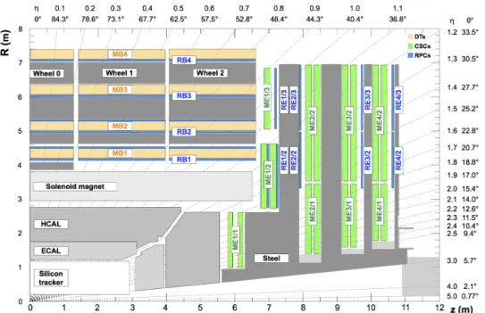
Figure 1: An R-z cross section of a quadrant of the CMS detector with the axis parallel to the beam (z) running horizontally and the radius (R) increasing upward. The interaction point is at the lower left corner. The locations of the various muon stations and the steel flux-return disks (dark areas) are shown. The drift tube stations (DTs) are labeled MB (“Muon Barrel”) and the cathode strip chambers (CSCs) are labeled ME (“Muon Endcap”). Resistive plate chambers (RPCs) are mounted in both the barrel and endcaps of CMS, where they are labeled RB and RE, respectively.
Three types of gas ionization chambers were chosen to make up the CMS muon system: drift tube chambers (DTs), cathode strip chambers (CSCs), and resistive plate chambers (RPCs). A detailed description of these chambers, including gas composition and operating voltage, can be found in Ref. [1]. The DTs are segmented into drift cells; the position of the muon is de-termined by measuring the drift time to an anode wire of a cell with a shaped electric field. The CSCs operate as standard multi-wire proportional counters but add a finely segmented cathode strip readout, which yields an accurate measurement of the position of the bending plane (R-φ) coordinate at which the muon crosses the gas volume. The RPCs are double-gap chambers operated in avalanche mode and are primarily designed to provide timing informa-tion for the muon trigger. The DT and CSC chambers are located in the regions|η| <1.2 and
0.9 < |η| < 2.4, respectively, and are complemented by RPCs in the range|η| < 1.9. We
dis-tinguish three regions, naturally defined by the cylindrical geometry of CMS, referred to as the barrel (|η| < 0.9), overlap (0.9< ||η|| <1.2), and endcap (1.2 < |η| < 2.4) regions. The
cham-bers are arranged to maximize the coverage and to provide some overlap where possible. An event in which two muons are reconstructed, one in the barrel and one in the endcap, is shown in Fig. 2.
In the barrel, a station is a ring of chambers assembled between two layers of the steel flux-return yoke at approximately the same value of radius R. There are four DT and four RPC stations in the barrel, labeled MB1–MB4 and RB1–RB4, respectively. Each DT chamber consists of three “superlayers”, each comprising four staggered layers of parallel drift cells. The wires in each layer are oriented so that two of the superlayers measure the muon position in the bending plane φ) and one superlayer measures the position in the longitudinal plane
3
Figure 2: A pp collision event with two reconstructed muon tracks superimposed on a cutaway image of the CMS detector. The image has been rotated around the y axis, which makes the inner tracker appear offset relative to its true position in the center of the detector. The four layers of muon chambers are interleaved with three layers of the steel flux-return yoke. The reconstructed invariant mass of the muon pair is 2.4 TeV. One muon is reconstructed in the barrel with a transverse momentum (pT) of 0.7 TeV, while the second muon is reconstructed in
the endcap with pT of 1.0 TeV.
RPC barrel stations, RB1 and RB2, are instrumented with two layers of RPCs each, facing the innermost and outermost sides of the DT. For stations 3 and 4 the RPCs have only one detection layer. The RPC strips are oriented parallel to the wires of the DT chambers that measure the coordinate in the bending plane. From the readout point of view, every RPC is subdivided into two or three η partitions called “rolls” [5]. Both DT and RPC barrel stations are arranged in five “wheels” along the z dimension, with 12 φ-sectors per wheel.
In the endcap, a station is a ring of chambers assembled between two disks of the steel flux-return yoke at approximately the same value of z. There are four CSC and four RPC stations in each endcap, labeled ME1–ME4 and RE1–RE4, respectively. Between Run 1 and Run 2, additional chambers were added in ME4 and RE4 to increase redundancy, improve efficiency, and reduce misidentification rates. Each CSC chamber consists of six staggered layers, each of which measures the muon position in two coordinates. The cathode strips are oriented radially to measure the muon position in the bending plane (R-φ), whereas the anode wires provide a coarse measurement in R. The RPC strips are oriented parallel to the CSC strips to measure the coordinate in the bending plane, and each endcap chamber is divided into three|η|partitions
(rolls) identified by the letters A, B, and C. In the radial direction, stations are arranged in two or three ”rings” of endcap RPCs and CSCs. In the inner rings of stations 2, 3, and 4, each CSC chamber subtends a φ angle of 20◦; all other CSCs subtend an angle of 10◦.
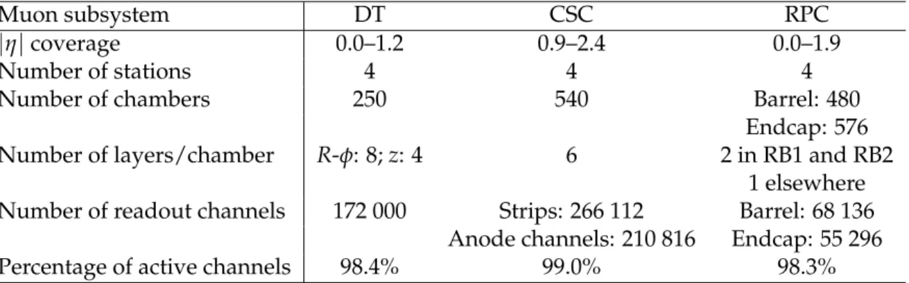
Table 1: Properties and parameters of the CMS muon subsystems during the 2016 data collec-tion period.
Muon subsystem DT CSC RPC
|η|coverage 0.0–1.2 0.9–2.4 0.0–1.9
Number of stations 4 4 4
Number of chambers 250 540 Barrel: 480
Endcap: 576 Number of layers/chamber R-φ: 8; z: 4 6 2 in RB1 and RB2
1 elsewhere Number of readout channels 172 000 Strips: 266 112 Barrel: 68 136
Anode channels: 210 816 Endcap: 55 296 Percentage of active channels 98.4% 99.0% 98.3%
Using these conventions, in this paper the performance of the DTs is specified according to chamber type, labeled “MBn±w”, where n is the barrel station (increasing with R), + or −
specifies the z-direction, and w is the wheel (increasing with|z|, with w = 0 centered at z= 0). The CSCs are labeled “ME±n/m”, where + or − specifies the z-direction, n is the endcap station (increasing with |z|), and m is the ring (increasing with R). If no sign is specified, the performance of the+ and − stations are combined. The inner ring of the CSC chambers in station 1 has a structure that is different from the other rings; the primary difference is an additional division of ME1/1 into two η partitions called a and b [1]. An overview of the number of chambers per chamber type, number of readout channels, and number of active channels in 2016 is given in Table 1.
The CMS trigger system consists of two stages [6] and is described in more detail in Section 9. A level-1 (L1) trigger based on custom-made electronics reduces the event rate from 40 MHz (LHC bunch crossing rate) to a readout rate of 100 kHz. For the muon component of the L1 trigger, CSC and DT chambers provide “trigger primitives” constructed from hit patterns con-sistent with muons that originate from the collision region, and RPC chambers provide hit information. When a specific bunch crossing is selected by the L1 algorithms as a potential event, readout of the precision data from the CMS detector is initiated via the “L1-Accept” (L1A) signal, which is synchronously distributed to all CMS subsystems. The high-level trig-ger (HLT), based on a farm of microprocessors, uses the precision data to reconstruct events to further reduce the rate of data to preserve for offline analysis to approximately 1 kHz. Both L1 and HLT use information from the muon system to efficiently identify muons over the broad energy range required for physics signatures of interest while minimizing the trigger rate and operating within the available latency.
The LHC is a bunched machine, in which the accelerated protons are distributed in bunches separated by one or more time steps of 25 ns. The running conditions of the LHC have evolved continuously since the beginning of its operation, and are expected to continue to evolve in the future [7–9]. As a representative comparison, we compare the LHC conditions in fill 1440 (Oc-tober 2010), included in the dataset analyzed in Refs. [1, 2], with the conditions in fill 5013 (June 2016), included in the 2016 data used in this paper. Between these two fills, the center-of-mass energy increased from√s = 7 TeV to√s = 13 TeV. The maximum instantaneous luminosity increased by about a factor of 40, from 2×1032cm−2s−1 to 8×1033cm−2s−1, as a result of the increases in both the number of colliding bunches and the luminosity per bunch. The number of colliding bunches increased by about a factor of 6, from 348 to 2028, facilitated by the re-duction of the spacing between proton bunches from 150 ns to 25 ns. The average luminosity per bunch increased by about a factor of 6.5, from 0.6×1030cm−2s−1 to 3.9×1030cm−2s−1, as
5
a result of several changes including increasing the number of protons per bunch, reducing the transverse widths of the beams, and focusing the beams more tightly [8, 9]. The combined increases in collision energy and luminosity per bunch caused the average number of inelastic collisions per crossing (pileup) to increase by about a factor of 8, from 3.6 to 28.
In order to prepare for these challenging LHC conditions and to exploit the corresponding gain in luminosity, the CMS muon system was significantly modified between Run 1 and Run 2. As mentioned previously, additional RPC and CSC chambers, RE4 and ME4/2, were installed in the fourth station to increase redundancy, improve efficiency, and reduce misidentification rates. The trigger and readout electronics were improved as part of the CMS-wide trigger upgrade [10], including optical links in the DTs and CSCs to increase bandwidth and to ease maintenance [11, 12]. New electronics were installed in the CSC ME1/1 chambers to read out every strip in the ME1/1a ring, covering 2.1< |η| <2.4. These strips had been ganged together
in Run 1, combining every 16th strip, which led to a 3-fold ambiguity for the position of a hit on that strip plane. The removal of the strip ganging in Run 2 leads to reduced capacitance, in turn leading to reduced noise and a resulting improvement in the φ resolution in ME1/1a.
3
Muon reconstruction
3.1 Hit and segment reconstruction
This section gives a brief overview of the “local” reconstruction algorithms in the CMS muon detector. Local reconstruction uses information from only a single muon chamber (RPC, CSC, or DT) to specify the passage of a muon through the chamber [1].
Muons and other charged particles that traverse a muon subdetector ionize the gas in the cham-bers, which eventually causes electric signals to be produced on the wires and strips. These signals are read out by electronics and are associated with well-defined locations, generically called “hits”, in the detector. The precise location of each hit is reconstructed from the electronic signals using different algorithms depending on the detector technology.
Hit reconstruction in a DT drift cell specifies the transverse distance between the wire and the intersection of the muon trajectory with the plane containing the wires in the layer. The electrons produced through gas ionization by a muon crossing the cell are collected at the anode wire. A time-to-digital converter (TDC) registers their arrival time, TTDC. This time is then
corrected by a time pedestal, Tped, and multiplied by the electron drift velocity, v, to reconstruct
the position of the DT hit:
position= (TTDC−Tped) ×v. (1)
The DT drift cell was designed to provide a uniform electric field so that the drift velocity can be assumed to be mostly constant for tracks impinging on the cell perpendicular to the plane of wires. The effect of deviations from this assumption on the spatial resolution is described in Section 5. In Equation 1, the time pedestal accounts for the time from the bunch crossing until the trigger decision arrives at the chamber electronics. It includes the time-of-flight (at the speed of light) along a straight line from the interaction region to the center of the wire, the average signal propagation time along the wire, the generation of trigger primitives, the processing by the L1 trigger electronics, the distribution of the L1A signals, and the receipt of L1A back at the readout electronics on the chamber. It also includes a wire-by-wire compo-nent that takes into account the different signal paths within a chamber. In another iteration, the time-of-flight and signal propagation time are refined using the segment position from the orthogonal superlayer available for MB1, MB2, and MB3. The calibration of Tped and v is
muons that cross the chamber at the location of the wire.
Hit reconstruction in a CSC layer measures the position of the traversing muon by combining information from the cathode strips and anode wires. The strips are radial, each subtending an angle of about 3 mrad (different chamber types have different angular strip widths that range from 2.2 to 4.7 mrad) and can thus accurately measure the φ angle. This is the bending direction of a muon traveling through the endcaps. In the endcaps the solenoidal field is first parallel to the z direction but then diverges radially, so a muon is first deflected in one azimuthal direction and then deflected in the opposite direction, with the maximum deflection occurring in the first station. The wires are orthogonal to the strips, except in ME1/1 where they are tilted to compensate for the Lorentz drift of ionization electrons in the non-negligible magnetic field in this region. They are ganged into wire groups of about 1–2 cm width, which results in a coarser-grained measurement in the radial direction. A CSC hit is reconstructed at the intersection points of hit strips and wire groups. A CSC reconstructed hit also has a measured time, which is calibrated such that hits from muons produced promptly in the triggering bunch crossing have a time distribution centered around zero.
Hit reconstruction in an RPC chamber requires clustering of hit strips. A charged particle pass-ing through the RPC produces an avalanche of electrons in the gap between two plates. This charge induces a signal on an external strip readout plane to identify muons from collision events with a precision of a few ns. The strips are aligned with η with up to 2 cm strip pitch, therefore giving a few cm spatial resolution in the φ coordinate. Since the ionization charge from a muon can be shared by more than one strip, adjacent strips are clustered to reconstruct one hit. An RPC hit is reconstructed as the strip cluster centroid.
While the RPC chambers are single-layer chambers, the CSC and DT chambers are multi-layer detectors where hits are reconstructed in each layer. From the reconstructed hits, straight-line track “segments” are built within each CSC or DT chamber.
Segment reconstruction in the DTs was modified prior to Run 2 [13]. The calibration of Tped
in Eq. 1 implicitly assumes that all muons take the same time to reach the reconstructed hit position from the interaction region. However, this assumption is not exactly true since hits could come from muons originating from other bunch crossings (“out-of-time muons”), or could be produced by heavy particles that travel at a reduced speed. Any such shift in the muon crossing time would cause all hits produced within a chamber to be shifted in space by the same amount. Therefore, DT segment reconstruction was modified prior to Run 2 to include time as third parameter, in addition to the intercept and slope of the standard two-dimensional straight-line pattern recognition and fit algorithm (in the plane transverse to the wire direction). The inclusion of time into segment reconstruction allows spurious early hits, produced by delta rays, to be removed from the segment reconstruction and thus improves the spatial resolution (see Section 5). The segment time information is not needed in the muon track reconstruction algorithm because of the negligible rate of accidentally matching out-of-time segments. The timing data are, however, kept with the reconstructed muon track information to be used in physics analyses (see Section 8).
3.2 Muon track reconstruction
In the standard CMS reconstruction procedure for pp collisions [2, 14, 15], tracks are first recon-structed independently in the inner tracker (tracker track) and in the muon system (standalone-muon track), and then used as input for (standalone-muon track reconstruction.
3.2 Muon track reconstruction 7
each with slightly different logic. After each iteration step, hits that have been associated with reconstructed tracks are removed from the set of input hits to be used in the following step. This approach maintains high performance and reduces processing time [14].
Standalone-muon tracks are built by exploiting information from muon subdetectors to gather all CSC, DT, and RPC information along a muon trajectory using a Kalman-filter technique [16]. Reconstruction starts from seeds made up of groups of DT or CSC segments.
Tracker muon tracks are built “inside-out” by propagating tracker tracks to the muon system with loose matching to DT or CSC segments. Each tracker track with transverse momentum pT >0.5 GeV and a total momentum p>2.5 GeV is extrapolated to the muon system. If at least
one muon segment matches the extrapolated track, the tracker track qualifies as a tracker muon track. The track-to-segment matching is performed in a local (x,y) coordinate system defined in a plane transverse to the beam axis, where x is the better-measured coordinate (in the
R-φplane) and y is the coordinate orthogonal to it. The extrapolated track and the segment are
matched either if the absolute value of the difference between their positions in the x coordinate is smaller than 3 cm, or if the ratio of this distance to its uncertainty (pull) is smaller than 4. Global muon tracks are built “outside-in” by matching standalone-muon tracks with tracker tracks. The matching is done by comparing parameters of the two tracks propagated onto a common surface. A combined fit is performed with the Kalman filter using information from both the tracker track and standalone-muon track.
Owing to the high efficiency of the tracker track and muon segment reconstruction, about 99% of the muons produced within the geometrical acceptance of the muon system are re-constructed either as a global muon track or as a tracker muon track, and very often as both. Global muons and tracker muons that share the same tracker track are merged into a single candidate.
Tracker muons have high efficiency in regions of the CMS detector with less instrumentation (for routing of detector services) and for muons with low pT. The tracker muons that are not
global muons typically match only to segments in the innermost muon station, but not other stations. This increases the probability of muon misidentification since hadron shower rem-nants can reach this innermost muon station (punch-through). Global muon reconstruction, which uses standalone-muon tracks, is designed to have high efficiency for muons penetrating through more than one muon station, which reduces the muon misidentification rate compared to tracker muons. By fully exploiting the information from both the inner tracker and the muon system, the pTmeasurement of global muons is also improved compared to tracker muons,
es-pecially for pT > 200 GeV. Muons reconstructed only as standalone-muon tracks have worse
momentum resolution and a higher admixture of cosmic muons than global or tracker muons. Reconstructed muons are fed into the CMS particle flow (PF) algorithm [17]. The algorithm combines information from all CMS subdetectors to identify and reconstruct all individual particles for each event, including electrons, neutral hadrons, charged hadrons, and muons. For muons, PF applies a set of selection criteria to candidates reconstructed with the standalone, global, or tracker muon algorithms. The requirements are based on various quality parameters from the muon reconstruction (described in Section 3.3), as well as make use of information from other CMS subdetectors (e.g., isolation as described in Section 3.5).
Prior to Run 2, two muon-specific calculations were added to the tracker track reconstruction to keep reconstruction and identification efficiency as high as possible under high-pileup con-ditions [17]. In the first calculation, tracker tracks identified as tracker muons are rebuilt by relaxing some quality constraints to increase track hit efficiency. In the second,
standalone-muon tracks with pT > 10 GeV that fulfill a minimal set of quality requirements are used to
seed an outside-in inner tracking reconstruction step. This additional set of tracks is combined with those provided by the inner tracking system and is exploited to build global and tracker muons.
3.3 Muon identification
A set of variables was studied and selection criteria were defined to allow each analysis to tune the desired balance between efficiency and purity. Some variables are based on muon recon-struction, such as track fit χ2, the number of hits per track (either in the inner tracker or in the muon system, or both), or the degree of matching between tracker tracks and standalone-muon tracks (for global standalone-muons). The standalone-muon segment compatibility is computed by propagating the tracker track to the muon system, and evaluating both the number of matched segments in all stations and the closeness of the matching in position and direction [15]. The algorithm returns values in a range between 0 and 1, with 1 representing the highest degree of compatibil-ity. A kink-finding algorithm splits the tracker track into two separate tracks at several places along the trajectory. For each split the algorithm makes a comparison between the two sepa-rate tracks, with a large χ2indicating that the two tracks are incompatible with being a single track. Other variables exploit inputs from outside the reconstructed muon track, such as com-patibility with the primary vertex (the reconstructed vertex with the largest value of summed physics-object p2T [18]). Using these variables, the main identification types of muons used in CMS physics analyses include:
• Loose muon identification (ID) aims to identify prompt muons originating at the pri-mary vertex, and muons from light and heavy flavor decays, as well as maintain a low rate of the misidentification of charged hadrons as muons. A loose muon is a muon selected by the PF algorithm that is also either a tracker or a global muon.
• Medium muon ID is optimized for prompt muons and for muons from heavy flavor decay. A medium muon is a loose muon with a tracker track that uses hits from more than 80% of the inner tracker layers it traverses. If the muon is only recon-structed as a tracker muon, the muon segment compatibility must be greater than 0.451. If the muon is reconstructed as both a tracker muon and a global muon, the muon segment compatibility need only be greater than 0.303, but then the global fit is required to have goodness-of-fit per degree of freedom (χ2/dof) less than 3, the position match between the tracker muon and standalone-muon must have χ2<12, and the maximum χ2computed by the kink-finding algorithm must be less than 20. The constraints on the segment compatibility were tuned after application of the other constraints to target an overall efficiency of 99.5% for muons from simulated W and Z events.
• Tight muon ID aims to suppress muons from decay in flight and from hadronic punch-through. A tight muon is a loose muon with a tracker track that uses hits from at least six layers of the inner tracker including at least one pixel hit. The muon must be reconstructed as both a tracker muon and a global muon. The tracker muon must have segment matching in at least two of the muon stations. The global muon fit must have χ2/dof < 10 and include at least one hit from the muon system. A tight muon must be compatible with the primary vertex, having a transverse impact parameter|dXY| <0.2 cm and a longitudinal impact parameter|dz| <0.5 cm.
• Soft muon ID is optimized for low-pTmuons for B-physics and quarkonia analyses. A
soft muon is a tracker muon with a tracker track that satisfies a high purity flag [14] and uses hits from at least six layers of the inner tracker including at least one pixel
3.4 Determination of muon momentum 9
hit. The tracker muon reconstruction must have tight segment matching, having pulls less than 3 both in local x and in local y. A soft muon is loosely compatible with the primary vertex, having|dXY| <0.3 cm and|dz| <20 cm.
• High momentum muon ID is optimized for muons with pT > 200 GeV. A high
mo-mentum muon is reconstructed as both a tracker muon and a global muon. The requirements on the tracker track, the tracker muon, and the transverse and longitu-dinal impact parameters are the same as for a tight muon, as well as the requirement that there be at least one hit from the muon system for the global muon. However, in contrast to the tight muon, the requirement on the global muon fit χ2/dof is re-moved. The removal of the χ2requirement prevents inefficiencies at high pTwhen
muons radiate large electromagnetic showers as they pass through the steel flux-return yoke, giving rise to additional hits in the muon chambers. A requirement on the relative pTuncertainty, σ(pT)/pT <30%, is used to ensure a proper momentum
measurement.
3.4 Determination of muon momentum
The default algorithm used by CMS to determine the muon momentum is the Tune-P algo-rithm [2]. For each muon, the Tune-P algoalgo-rithm selects the pT measurement from one of the
following refits based on goodness-of-fit information and σ(pT)/pT criteria to reduce tails in
the momentum resolution distribution due to poor quality fits.
• Inner-Track fit determines the momentum using only information from the inner tracker. While various fit methods are used to add information from the muon de-tector to improve the measurement of the momentum at high pT, for muons with
pT < 200 GeV, the contribution from the muon system to the momentum
measure-ment is marginal. Therefore, the inner-track fit is highly favored by Tune-P at low momentum.
• Tracker-Plus-First-Muon-Station fit starts with the hits from the global muon track and performs a refit using only information from the inner tracker and the innermost muon station containing hits. The innermost station provides the best information about momentum within the muon system.
• Picky fit aims at properly determining the momentum for events in which shower-ing occurred within a chamber. This algorithm again starts with the hits from the global muon track, but in chambers that have a large hit occupancy (i.e. likely from a shower) the refit uses only the hits that are compatible with the extrapolated tra-jectory (based on χ2).
• Dynamic-Truncation fit accounts for cases when energy losses cause significant bend-ing of the muon trajectory. The algorithm propagates the tracker track to the inner-most station and performs a refit adding hits from the segment closest to the extrap-olated trajectory, if compatible. Starting from the refit, the algorithm is repeated for each station propagating outward. If no compatible hit is found in two consecutive muon stations, the algorithm stops.
The Tune-P algorithm was validated using cosmic ray muons, muons from pp collisions, and Monte Carlo simulations generated using different misalignment scenarios. Both the core and the tails of the momentum, curvature, and invariant mass distributions were studied to ensure that no significant biases in the muon momentum assignment are introduced by the algorithm. The PF algorithm refines the information from Tune-P, exploiting information from the full
event, by selecting refits that significantly improve the balance of missing pT and by using
a post-processing algorithm designed to preserve events that contain genuine missing en-ergy [17]. The PF momentum assignment was also validated using Monte Carlo simulation and muons from pp collisions.
3.5 Muon isolation
To distinguish between prompt muons and those from weak decays within jets, the isolation of a muon is evaluated relative to its pT by summing up the energy in geometrical cones,
∆R= √
(∆φ)2+ (∆η)2, surrounding the muon. One strategy sums reconstructed tracks (track based isolation), while another uses charged hadrons and neutral particles coming from PF (PF isolation).
For the computation of PF isolation [17], the pTof charged hadrons within the∆R cone
originat-ing from the primary vertex are summed together with the energy sum of all neutral particles (hadrons and photons) in the cone. The contribution from pileup to the neutral particles is corrected by computing the sum of charged hadron deposits originating from pileup vertices, scaling it by a factor of 0.5, and subtracting this from the neutral hadron and photon sums to give the corrected energy sum from neutral particles. The factor of 0.5 is estimated from simulations to be approximately the ratio of neutral particle to charged hadron production in inelastic proton-proton collisions. The corrected energy sum from neutral particles is limited to be positive or zero.
For both strategies, tight and loose working points are defined to achieve efficiencies of 95% and 98%, respectively. They are tuned using simulated tight muons from Z → µ+µ− decays
with pT > 20 GeV. The values for the tight and loose working points for PF isolation within
∆R<0.4 are 0.15 and 0.25, respectively, while the values for track based isolation within∆R<
0.3 are 0.05 and 0.10. The efficiency of the working points to reject muons in jets was tested in simulated multi-jet QCD events (events comprised uniquely of jets produced through the strong interaction) and simulated events containing a W boson plus one or more jets (W+jets).
4
Data and simulated samples
Results shown in this paper come from one of two data sets: approximately 2 fb−1 of pp col-lisions collected in 2015, which will be called “2015 data”, and approximately 4 fb−1 of pp collisions collected in 2016, which will be called “2016 data”. The data set that was used for each result in this paper was chosen depending on the availability of the data and the analyst. In any case, the results represent the CMS muon performance in Run 2 no matter which data set is used, since the peak luminosity delivered by LHC in 2015 and 2016 differed only by about a factor of three, which is small compared to the factor of 40 difference between 2010 and 2016 as described in Section 2. The selected data samples consist of events with a pair of reconstructed muons with low pT thresholds. Further event criteria are applied depending on the analyses
performed, and are described in detail later.
The performance results most directly applicable to physics analyses are presented in this pa-per using the 2015 data. These data are compared with simulations from several Monte Carlo event generators for signal and background processes. The Drell-Yan Z/γ∗ →l+l−signal sam-ple is generated at next-to-leading order (NLO) with MADGRAPH5 [email protected] [19]. The background samples of W+jets and of tt pairs with one or more jets (tt +jets) are also produced with the same generator. The background from single top quark tW production is generated at NLO with POWHEG v1.0 [20]. ThePYTHIA 8.212 [21, 22] package is used for QCD events
11
enriched in muon decays, parton showering, hadronization, and simulation of the underlying event via tune CUETP8M1 [23], using NNPDF2.3 LO [24] as the default set of parton distribu-tion funcdistribu-tions. For all processes, the detector response is simulated using a detailed descripdistribu-tion of the CMS detector based on the GEANT4 package [25] and event reconstruction is performed
with the same algorithms as used for the data. The simulated samples include pileup, and the events are weighted so that the pileup distribution matches the 2015 data, having an average pileup of about 11.
5
Spatial resolution
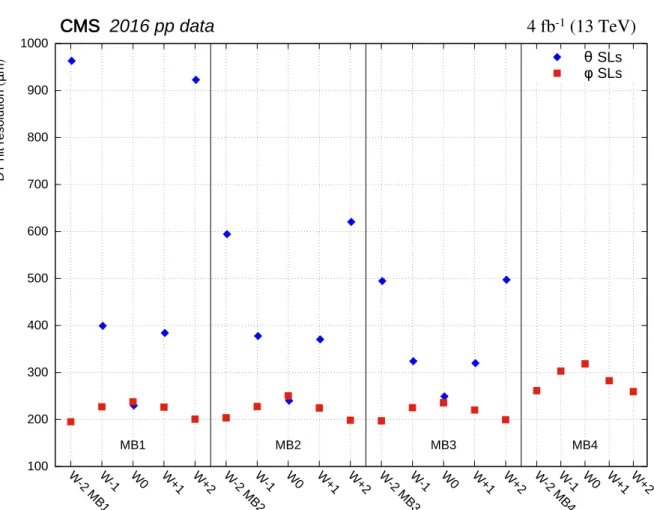
The spatial resolution of a muon subdetector is quantified by the width of the distribution of residuals between the reconstructed and expected hit positions. The expected position is estimated from the segment fit. The resolution is obtained from the residual width by applying standard analytical factors calculated from the “hat matrix” that relates the residuals from a fit to the fitted measurements, and hence the widths of the residual distributions to the intrinsic resolution of the measurements [26]. These factors differ for CSC, in which the reconstructed hit used for the residual is excluded from the segment fit, and for DT where the hit is included. Both CSCs and DTs are designed to make a precise measurement in the direction of bending of a muon track because this directly affects the measurement of the momentum. This is the azimuthal direction, measured in the CSCs by the strips, and in the DTs by the φ superlayers. The spatial resolution of the DTs is determined by computing the value of the residual for each hit used to reconstruct each segment. Typically, eight residual values are computed for each
φsegment and four for each θ segment. Due to the azimuthal symmetry of the DTs, a single
residual distribution is filled with all hits having the same wire orientation from all chambers in the same wheel and station. The width of each residual distribution is converted to position resolution using the standard analytically computed factors described above. Figure 3 shows the spatial resolution of DT hits sorted by station, wheel, and wire orientation. The resolution in the φ superlayers (i.e., in the bending plane) is better than 250 µm in MB1, MB2 and MB3, and better than 300 µm in MB4. In the θ superlayers, the resolution varies from about 250 to 600 µm except in the outer wheels of MB1.
Within every station, both θ and φ superlayers show symmetric behavior with respect to the z = 0 plane, as expected from the detector symmetry. In wheel 0, where tracks from the in-teraction region are mostly perpendicular to all layers, the resolution is the same for θ and φ superlayers. From wheel 0 toward the forward region, tracks from the interaction region have increasing values of|η|; this affects θ and φ superlayers in opposite ways. In the θ
superlay-ers the increasing inclination angle degrades the linearity of the distance-drift time relation, thus worsening the resolution. In contrast, in φ superlayers the inclination angle increases the track path within the tube (along the wire direction), thus increasing the ionization charge and improving the resolution. The resolution of the φ superlayers is worse in MB4 because no θ measurement is available, so no corrections can be applied to account for the muon time of flight and the signal propagation time along the wire. The DT spatial resolution in the 2016 data is improved by about 10% compared to the 2010 results [1] as a result of the improved track reconstruction method in Run 2 that removes spurious early hits, produced by delta rays, from the segment reconstruction (see Section 3.1).
The spatial resolution of the CSCs is studied using locally reconstructed segments that have exactly one hit per layer. For each segment, the hit in one layer is dropped and the segment is re-fitted with the remaining five hits. The residual between the dropped hit and the new fit is calculated as R∆φ in the R-φ plane, which is the precision coordinate measured by the strips
100 200 300 400 500 600 700 800 900 1000 W -2 MB 1 W -1 W0 W+1 W+2 W-2 MB 2 W -1 W0 W+1 W+2 W-2 MB 3 W -1 W0 W+1 W+2 W-2 MB 4 W -1 W0 W+1W+2 MB1 MB2 MB3 MB4 DT h it resolution (µ m ) CMS 2016 pp data 4 fb-1 (13 TeV) θ SLs φ SLs
Figure 3: Reconstructed hit resolution for DT φ superlayers (squares) and DT θ superlayers (diamonds) measured with the 2016 data, plotted as a function of station and wheel. The un-certainties in these values are smaller than the marker size in the figure.
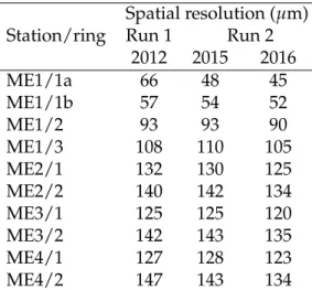
and the direction of the magnetic bending of the muon. This procedure is repeated for each layer. These residuals are approximately Gaussian and the residual widths are converted to position resolution by using standard analytical factors [26]. The spatial resolution of the CSC strip measurement depends on the relative position at which a muon crosses a strip: it is better for a muon crossing near a strip edge than at the center because then more of the induced charge is shared between that strip and its neighbor, allowing a better estimate of the center of the charge distribution. To benefit from this fact, alternate layers in a CSC are staggered by half a strip width, except in the ME1/1 chambers where the strips are narrower and the effect is small. Resolutions are measured separately for the central half of a strip width (σC)
and the quarter strip-width at each edge (σE) [1]. The layer measurements are combined to
give an overall resolution σ per CSC station by 1/σstation2 = 6/σlayer2 (ME1/1 chambers) and 1/σstation2 = 3/σC2 +3/σE2 (chambers other than ME1/1). Table 2 summarizes the mean spatial resolution in each CSC station and ring. The design specifications for the spatial resolutions in the CSC system were 75 µm for ME1/1 chambers and 150 µm for the others. These resolutions were chosen so that the contribution of the chamber spatial resolution to the muon momentum resolution is less than or comparable to the contribution of multiple scattering.
The precision of the CSC measurements is dominated by systematic effects, and the statistical uncertainties arising from the fits to the residual distributions are small (<0.2%). The preci-sion is controlled by the size of the induced charge distribution on the strip plane, which is
13
Table 2: CSC transverse spatial resolution per station (6 hits) measured for all chamber types with 2016 data, compared to those measured in 2015 and 2012.
Spatial resolution (µm) Station/ring Run 1 Run 2
2012 2015 2016 ME1/1a 66 48 45 ME1/1b 57 54 52 ME1/2 93 93 90 ME1/3 108 110 105 ME2/1 132 130 125 ME2/2 140 142 134 ME3/1 125 125 120 ME3/2 142 143 135 ME4/1 127 128 123 ME4/2 147 143 134
affected by geometry (the width of the strips), gas gain (high voltage, gas mix, gas pressure), and sample selection (momenta, angle of incidence). The gas mix and high voltage are strin-gently maintained constant during CSC operation, and muon samples are selected to be as close as possible for the purposes of these comparisons. The CSCs operate at atmospheric pres-sure, but a decrease of atmospheric pressure of 1% increases the gas gain by approximately 7%, so the values in the table have all been normalized to 965 mbar, a value typical of the an-nual average atmospheric pressure at CMS. In this manner we obtain reproducible resolutions typically within 1–2 µm, as can be seen from the values in Tab. 2 for the columns for 2012 and 2015 (other than for ME1/1a). The approximately 25% improvement in resolution in ME1/1a CSCs between 2012 and later is because of the removal of the strip ganging that was used in the first CMS running periods. The improved resolution is not directly related to the spatial nature of the ganging—every 16th strip was ganged into a single channel, rather than combin-ing neighborcombin-ing strips. Instead, the improvement is because of the reduction of capacitance, and hence noise, with the removal of this ganging. The spatial resolution values for 2016 are systematically better than expected, and this was eventually traced to an incorrectly calibrated gas flowmeter that led to a slightly increased argon fraction in the gas mix in early 2016. Once this was corrected1the measured values returned to those seen in earlier running periods. The spatial resolution of the RPCs is studied by extrapolating segments from the closest CSC or DT to the plane of strips in the chamber under study. The residuals are calculated transverse to the direction of the strips, which is also the direction of the bending of muons in the magnetic field. The residual is defined as the transverse distance between the center of the reconstructed RPC cluster and the point of intersection of the extrapolated segment with the plane of strips. For each station and layer, a residual distribution is filled and fit with a Gaussian. The σ pa-rameter of these fits varies between 0.78–1.27 cm in the barrel and 0.89–1.38 cm in the endcap. These values are compatible with the resolution expected from the widths of the strips and are consistent with the 2010 results [1].
The spatial compatibility between tracker tracks, reconstructed with the inner tracker, and seg-ments, reconstructed in the muon chambers, is of primary importance and is extensively used
1Better spatial resolution is not the only consideration in choice of gas mix for CSC operation in CMS. The gas mix is just one of many parameters of the system design that were optimized to provide the required spatial resolution while maintaining stable and robust operation of the detectior and maximum longevity of the chambers in the LHC environment.
in the muon ID criteria presented in Section 3.2. The residuals between extrapolated tracker tracks and segments are studied using the tag-and-probe technique [2]. Oppositely charged dimuon pairs are selected from a sample collected with a single-muon trigger. The tag is a tight muon with tight PF isolation, which is geometrically matched with the trigger (∆R <0.1 between the tracker track and the 4-vector reconstructed by HLT). The probe is a tracker muon, which passes track-based isolation and tracker track quality requirements, that is propagated to each of the DT or CSC chambers it traverses. The segment matching in the definition of a tracker muon is loose enough not to bias this measurement.
The transverse residual, ∆x, is computed in the chamber local reference frame for the coor-dinate measuring the muon position in the bending plane (φ). It corresponds to the distance between the position of the propagated tracker track and the segment in the chamber. The RMS of the distribution of ∆x is shown in Fig. 4 for 2015 data and simulated Z/γ∗ → l+l− decays. There is reasonable agreement between the data and simulation. The alignment preci-sion of the data (using the techniques described in Ref. [27] with the full 2015 data set) and of the simulation (corresponding to what would be obtained with about 1 fb−1 of data) is about 100–200 µm, and thus is not a dominant effect in these results. Figures 4a and 4b show the RMS as a function of station for DT and CSC chambers, respectively. The RMS increases as the muon station number increases, which is expected because of the larger amount of material traversed by the muons and the resultant multiple scattering. The RMS of the residual eval-uated in the first muon station is shown as a function of momentum in Fig. 4c and Fig. 4e in the barrel and endcap regions, respectively, while Fig. 4d shows the overlap region between the two. The RMS decreases with momentum because of the reduction in multiple scattering. The spatial resolution in Fig. 4 is not directly comparable with the results in Ref. [2] because the analysis used on the 2015 data reduced the contamination from muons that do not come from the primary interaction.
6
Efficiency
6.1 Hit and segment efficiency
The hit reconstruction efficiency is calculated as the ratio of the number of reconstructed hits divided by the number of expected hits. The measurement provided by the detecting unit under study is excluded from the computation of the expected hit position.
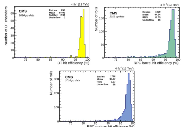
The hit reconstruction efficiency of the DTs is studied using segments. To ensure high quality segment reconstruction, segments are required to have at least one reconstructed hit in all layers except the layer under study. For the efficiency of a φ layer, this implies that the φ segment must have at least seven associated hits, while for θ layers, the θ segment must have at least three associated hits. In addition to the high quality of the segment in the view under study, there must be a segment constructed in both φ and θ views to ensure the presence of a genuine muon crossing the chamber. For φ superlayers, backgrounds are reduced by requiring the segment inclination to be smaller than 45◦(by construction, muons from the interaction region are mostly orthogonal to the wire plane). The intersection of this segment with the layer under study determines the position of the expected hit within a specific tube and increments the denominator in the efficiency calculation. The numerator is incremented if a hit is reconstructed in this tube. The distribution of the hit reconstruction efficiency for each DT chamber is shown in Fig. 5a. The average value of the DT hit reconstruction efficiency is 97.1% including the dead cells reported in Table 1. The average efficiency in the 2016 data is consistent with the 2010 average [1] within 1%.
6.1 Hit and segment efficiency 15 DT muon station MB1 MB2 MB3 MB4 x) (cm) ∆ RMS( 0 0.5 1 1.5 2 2.5 3 3.5 Data Simulation CMS 2015 pp data 2 fb-1 (13 TeV) CSC muon station
ME1 ME2 ME3 ME4
x) (cm) ∆ RMS( 0 0.5 1 1.5 2 2.5 Data Simulation CMS 2015 pp data 2 fb-1 (13 TeV) p (GeV) 10 102 103 x) (cm) ∆ RMS( 0 0.5 1 1.5 2 2.5 3 |η| < 0.9 Data Simulation CMS 2015 pp data 2 fb-1 (13 TeV) p (GeV) 10 102 103 x) (cm) ∆ RMS( 0 0.5 1 1.5 2 2.5 3 0.9 < |η| < 1.2 Data Simulation CMS 2015 pp data 2 fb-1 (13 TeV) p (GeV) 10 102 103 x) (cm) ∆ RMS( 0 0.5 1 1.5 2 2.5 3 1.2 < |η| < 2.4 Data Simulation CMS 2015 pp data 2 fb-1 (13 TeV)
Figure 4: The RMS of transverse residuals between reconstructed segments and propagated tracker tracks, measured in 2015 data. Results are plotted as a function of: (upper left) MB station in the DTs; (upper right) ME station in the CSCs; (lower left) momentum p in station 1 of the barrel region (|η| ≤ 0.9); (lower center) momentum p in station 1 of the overlap region
(0.9≤ |η| ≤1.2); (lower right) momentum p in station 1 of the endcap region (1.2≤ |η| ≤2.4).
The vertical error bars represent the statistical uncertainties of the RMS, and are smaller than the marker size for most data points.
The hit reconstruction efficiency of the RPCs is studied with a tag-and-probe technique. Muon pairs are selected from an event sample collected with a single-muon trigger. The tag is a tight muon that is geometrically matched with the trigger (∆R<0.1 between the tracker track and the 4-vector reconstructed by HLT). The probe is a tracker muon matched to a DT or CSC segment that is extrapolated to RPC chambers. For each RPC roll that the extrapolated probe traverses, the denominator in the efficiency calculation is incremented and a matching hit is sought. The numerator is incremented if the absolute value of the difference between the hit position and the extrapolated probe position is smaller than 10 cm, or if the ratio of this dis-tance to its uncertainty (pull), including the extrapolation uncertainty, is less than 4. Figures 5b and c show the efficiency for all RPC barrel and endcap rolls, respectively. The average hit ef-ficiency is 94.2% for the RPC barrel and 96.4% for the RPC endcaps, with negligible accidental contributions from noise. The underflow entries are from rolls with efficiency lower than 70% caused by known hardware problems: chambers with gas leaks in the barrel, and low voltage problems in the endcap. The rolls with zero efficiency (Tab. 1) are included in the underflow and the average efficiency. Results on RPC hit efficiency from 2010 [1] and 2016 are consistent within 1%.
Muons rarely fail to traverse an entire CSC so the CSC readout system [3] requires hits com-patible with a charged track crossing a chamber, which suppresses readout of hits from several
Entries 250 Mean 97.05 Std Dev 2.93 Underflow 0 DT hit efficiency (%) 75 80 85 90 95 100 Number of DT chambers 0 10 20 30 40 50 60 Entries 250 Mean 97.05 Std Dev 2.93 Underflow 0 CMS 2016 pp data (13 TeV) -1 4 fb
RPC barrel hit efficiency (%)
75 80 85 90 95 100 Number of rolls 0 50 100 150 1020 94.24 11.55 43 4 fb-1 (13 TeV) Entries Mean RMS Underflow CMS 2016 pp data
RPC endcap hit efficiency (%)
75 80 85 90 95 100 Number of rolls 0 100 200 300 1728 96.37 5.57 39 4 fb-1 (13 TeV) Entries Mean RMS Underflow CMS 2016 pp data
Figure 5: Hit reconstruction efficiency measured with the 2016 data in (upper left) DT, (upper right) RPC barrel, and (lower) RPC endcap chambers.
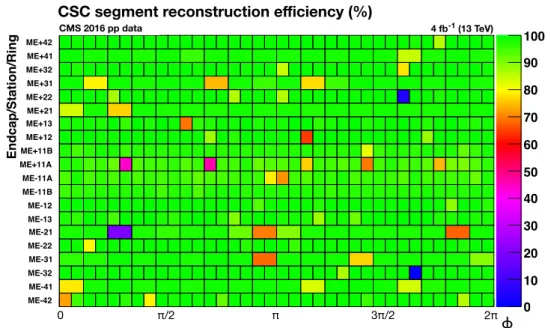
sources of uninteresting background. In order to read out a cathode front-end board, which services 16 strip channels in each of the six layers of a CSC, the basic pattern of hits expected for a CSC trigger primitive must occur in coincidence with a level-1 trigger from CMS. A trig-ger primitive requires at least 4 layers in a CSC containing strip hits, with a pattern consistent with those created by muons originating at the pp collision point. This readout suppression complicates the interpretation of straightforward measurements of CSC layer-by-layer hit effi-ciencies, but since the muon track reconstruction uses segments, and not individual hits, it is the segment efficiency that is most important to system operation. This can be directly mea-sured using the tag-and-probe method. The tag is required to be a tracker muon and the probe is a tracker track that is projected to the muon system. To reduce background and ensure that the probe actually enters the chamber under consideration, compatible hits are also required in a downstream CSC. In the case of station 4, an upstream segment is required. Figure 6 shows a summary map of the measured reconstructed segment efficiency for each CSC. The average CSC segment reconstruction efficiency is 97.4%. A few of the 540 chambers have known in-efficiencies, usually caused by one or more faulty electronics boards that cannot be repaired without major intervention requiring the dismantling of the system. There are also occasional temporary failures of electronics boards that last for a few hours or days and can be recovered without major intervention. Both contribute to a reduced segment efficiency in a localized re-gion. The average CSC segment efficiency in the 2016 data is within 1% of that observed in 2010 [1].
6.2 Reconstruction, identification and isolation efficiency
The efficiency for muons is studied with the tag-and-probe method beginning with tracker tracks as probes. The value of the efficiency is computed by factorizing it into several compo-nents [2]:
6.2 Reconstruction, identification and isolation efficiency 17 0 10 20 30 40 50 60 70 80 90 100
CSC Segment Reconstruction Efficiency (%)
φ 0 π/2 π 3π/2 2π Endcap/Station/Ring ME-42 ME-41 ME-32 ME-31 ME-22 ME-21 ME-13 ME-12 ME-11B ME-11A ME+11A ME+11B ME+12 ME+13 ME+21 ME+22 ME+31 ME+32 ME+41 ME+42 -1 =13 TeV, L=4 fb s CMS Preliminary 2016
CSC Segment Reconstruction Efficiency (%)CSC segment reconstruction efficiency (%)
4 fb-1 (13 TeV) CMS 2016 pp data
0 π/2 π 3π/2 2π
ϕ
Figure 6: The efficiency (in percent) of each CSC in the CMS endcap muon detector to provide a locally reconstructed track segment as measured from 2016 data.
Each component of eµis determined individually. The efficiency of the tracker track
reconstruc-tion is etrack[14]. The reconstruction+ID efficiency, ereco+ID, contains both the efficiency of muon
reconstruction in the muon system, including the matching of this muon to the tracker track, and the efficiency of the ID criteria. The efficiency of muon isolation, eiso, is studied relative to
a probe that has passed the specified muon ID. The efficiency of the trigger, etrig, is described
in detail in Section 9.2. The application of Eq. 2 is dependent on the specific needs of each anal-ysis. For example, if an analysis does not require isolation, eisois removed from the equation
and etrigis computed relative to reconstructed muons without an isolation requirement.
As described in Ref. [2], the combinatorial background of tag-probe pairs not coming from the Z resonance (where the probe is usually a charged hadron misidentified as a muon) is sub-tracted by performing a simultaneous fit to the invariant mass spectra for passing and failing probes with identical signal shape and appropriate background shapes; the efficiency is then computed from the normalizations of the signal shapes in the two spectra. Given the high multiplicity of tracks in proton-proton collision events, using a tracker track as the probe leads to a high combinatorial background in low-pT bins, which can result in large uncertainties in
the background subtraction method. To mitigate this effect, the efficiency measurement is per-formed using only the tag-and-probe pairs for which a single probe is associated with the tag. The same method is also applied to simulated Z→µ+µ−events.
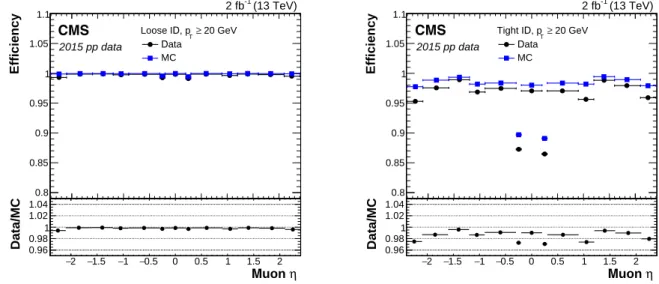
The ereco+ID for loose muons and for tight muons are shown as a function of η in Fig. 7, for
both data and simulation. The loose ID efficiency exceeds 99% over the entire η range, and the data and simulation agree to within 1%. As a function of pT between 20 GeV and 200 GeV
(where the efficiency is measured with reasonably small uncertainty), the loose ID efficiency is constant with fluctuations well within 1%. The tight ID efficiency varies between 95% and 99%, depending on η, and the data and simulation agree to within 1–3%. The dips in efficiency close to|η| = 0.3 are due to the regions with less instrumentation between the central muon
wheel and the two neighboring wheels. In Fig. 7b, the simulation is systematically higher than the data as a result of small imperfections in the model, which are revealed by the stringent requirements for a muon to satisfy tight ID criteria. In the endcap, differences between the data
18
and simulation arise when the muon is required to be global with a combined fit that has valid hits in the muon system, whereas in the barrel segment matching and global reconstruction contribute to the discrepancy in a similar way. Tracker track quality constraints contribute to a discrepancy of less than 0.5% over the full η range.
Efficiency 0.8 0.85 0.9 0.95 1 1.05 1.1 20 GeV ≥ T Loose ID, p Data MC 20 2 fb-1 (13 TeV) Muon η 2 − −1.5 −1 −0.5 0 0.5 1 1.5 2 Data/MC 0.96 0.98 1 1.02 1.04 CMS 2015 pp data Efficiency 0.8 0.85 0.9 0.95 1 1.05 1.1 20 GeV ≥ T Tight ID, p Data MC 20 2 fb-1 (13 TeV) Muon η 2 − −1.5 −1 −0.5 0 0.5 1 1.5 2 Data/MC 0.96 0.98 1 1.02 1.04 CMS 2015 pp data
Figure 7: Tag-and-probe efficiency for muon reconstruction and identification in 2015 data (cir-cles), simulation (squares), and the ratio (bottom inset) for loose (left) and tight (right) muons with pT > 20 GeV. The statistical uncertainties are smaller than the symbols used to display
the measurements.
A hadron may be misidentified as a prompt muon if the hadron decays in flight, or if hadron shower remnants penetrate through the calorimeters and reach the muon system (punch-through), or if there is a random matching between a hadron track in the inner tracker and a segment or standalone-muon in the muon system. The probability of hadrons to be misidentified as muons is measured by using data samples of pions and kaons from resonant particle decays collected with jet triggers [2]. The probability of pions to be misidentified as loose muons in both data and simulation is about 0.2% while for tight muons it is about 0.1%. In the same way, 0.5% of kaons are misidentified as loose muons and 0.3% as tight muons in both data and simulation. The uncertainty in these measurements is at the level of 0.05% and is dominated by the limited statistical precision. Within uncertainties, the misidentification probabilities are independent of pT. These results are in good agreement with Run 1.
The efficiency of muon isolation, eiso, is studied relative to a probe that passes a given muon
ID criteria. For example, the tight PF isolation efficiency relative to tight muons is shown in Fig. 8. In this case the agreement between the data and simulation is always better than 0.5%. Analogous to the misidentification probability study described above, the efficiency to incorrectly label muons within jets as being isolated is measured with simulated QCD events enriched in muon decays. In this sample, the probability of a muon with pT > 20 GeV that
fulfills the tight muon ID criteria to also satisfy tight isolation requirements is about 5% in the barrel, and goes up to about 15% in the endcap.
The systematic uncertainty in data/simulation scale factors for the efficiencies described above is estimated by varying the tag-and-probe conditions. The impact of the background contami-nation is estimated by using different requirements on the tag muon (pTand isolation) and on
the requirement of a single probe being associated with the tag. The dominant uncertainty is caused by the choice of the signal and background models used in the fits. It is estimated by testing alternative fit functions and by varying the range and the binning of the invariant-mass
6.2 Reconstruction, identification and isolation efficiency 19 Efficiency 0.8 0.85 0.9 0.95 1 1.05 1.1 Tight iso/Tight ID, η≤ 2.4 Data MC 20 40 60 80 100 120 140 160 180 200 220 2 fb-1 (13 TeV) (GeV) T Muon p 20 40 60 80 100 120 140 160 180 200 Data/MC 0.960.98 1 1.02 1.04 CMS 2015 pp data Efficiency 0.8 0.85 0.9 0.95 1 1.05 1.1 20 GeV ≥ T Tight iso/Tight ID, p Data MC 20 40 60 80 100 120 140 160 180 200 220 2 fb-1 (13 TeV) Muon η 2 − −1.5 −1 −0.5 0 0.5 1 1.5 2 Data/MC 0.960.98 1 1.02 1.04 CMS 2015 pp data
Figure 8: Tag-and-probe efficiency for the tight PF isolation working point on top of the tight ID (left) versus pTfor muons in the acceptance of the muon spectrometer, and (right) versus
pseu-dorapidity for muons with pT > 20 GeV, for 2015 data (circles), simulation (squares), and the
ratio (bottom inset). The statistical uncertainties are smaller than the symbols used to display the measurements.
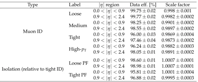
Table 3: Efficiencies for several reconstruction+ID algorithms and isolation criteria (relative to tight ID) for muons with pT >20 GeV. The corresponding scale factors are for 2015 data relative
to simulation. The uncertainties in the scale factors stem from the statistical uncertainties in the fitting procedure. Systematic uncertainties are described in the text.
Type Label |η|region Data eff. [%] Scale factor
Muon ID Loose 0.0< |η| <0.9 99.75±0.02 0.998±0.001 0.9< |η| <2.4 99.77±0.02 0.9982±0.0002 Medium 0.0< |η| <0.9 98.25±0.02 0.9901±0.0002 0.9< |η| <2.4 98.55±0.02 0.9897±0.0002 Tight 0.0< |η| <0.9 96.00±0.03 0.9869±0.0004 0.9< |η| <2.4 97.46±0.04 0.9873±0.0002 High-pT 0.0 < |η| <0.9 96.24±0.02 0.9882±0.0003 0.9< |η| <2.4 98.05±0.01 0.9891±0.0002
Isolation (relative to tight ID)
Loose PF 0.0< |η| <0.9 98.60±0.01 1.0007±0.0001 0.9< |η| <2.4 98.98±0.01 1.0007±0.0001
Tight PF 0.0< |η| <0.9 95.81±0.02 1.0001±0.0004 0.9< |η| <2.4 96.88±0.02 0.9995±0.0003
spectrum. The uncertainties are estimated to be at the level of 1% for ID and 0.5% for isolation. For muons with pT >20 GeV, Table 3 shows the data efficiency and the data/simulation scale
factors for the muon ID and isolation working points described in Section 3. For all entries, the agreement between data and simulation is better than 1.5%. The efficiencies, systematic uncertainties, and scale factors between data and simulation for 2015 are similar to those found in the 2010 data. The statistical uncertainties, however, have been reduced by a factor of 10 and become negligible in comparison with the systematic uncertainties.
7
Momentum scale and resolution
Many searches for new physics are characterized by signatures involving prompt muons with high pT. For muons with pT > 200 GeV, combining information from the muon system with
information from the inner tracker significantly improves the momentum measurement [28]. On the other hand, for muons with lower pT the momentum measurement is dominated by
the performance of the inner tracker. To assess the performance of the momentum scale and resolution, data from both cosmic rays and collisions have been analyzed.
7.1 Low and intermediate pT: scale and resolution with collisions
For muons with low and intermediate pT, two different methods are utilized in Run 2 to correct
the muon momentum scale and to estimate the resolution. One method derives the corrections from the mean value of the distribution of 1/pµT,1/pTµ , for tight muons from Z decays, with further tuning performed using the mean of the dimuon invariant mass spectrum, Mµµ [29].
Another method determines corrections using a Kalman filter on tight muons from J/ψ and Υ(1S) decays [30]. The magnitudes of the momentum scale corrections are about 0.2% and 0.3% in the barrel and endcap, respectively. After the scale is corrected, the resolution is de-termined either as a function of η (first method) or as a function of η and pT(second method),
including contributions from multiple scattering, position error, and additional smearing to make the simulation match the data. The resolution for muons with momenta up to approxi-mately 100 GeV is 1% in the barrel and 3% in the endcap. For both techniques, over all η and pT
values, the uncertainty in the resolution is estimated to be about 5% of its value. Compared to the 2010 results [2], the 2015 resolution has improved, primarily because of the improvements to the tracker alignment [27].
7.2 Momentum resolution with cosmic rays
Cosmic ray muons passing through the CMS detector are used to estimate the momentum resolution at high pTby comparing the momentum measured in the upper half of the detector
with the momentum measured in the lower half [2, 15]. Events are selected with muons that cross the detector close to the interaction point and have at least one hit in the pixel detector, so that each leg of the cosmic ray mimics a muon from a collision. To ensure good reconstruction, the tracker track of each muon leg is required to have at least one pixel hit as well as five strip layers. The relative q/pTresidual, R(q/pT), is computed as
R(q/pT) = 1 √ 2 (q/pT)upper− (q/pT)lower (q/pT)lower , (3)
where q is the muon charge, and upper and lower refer to the muon tracks reconstructed in the upper and lower halves of the CMS detector, respectively. The quantity q/pT, proportional to
the muon trajectory curvature, has a symmetric, approximately Gaussian, resolution distribu-tion. The factor of √2 accounts for the fact that the q/pT measurements of the two tracks are
independent.
Figure 9 shows the RMS of R(q/pT)as a function of pT for cosmic rays recorded in 2015 for
fits using only the inner tracker and for fits that include the muon system using the Tune-P algorithm. The uncertainty in the last bins is dominated by the small number of cosmic rays collected in 2015 (66 events with pT > 500 GeV). The improvement in resolution from
exploit-ing the muon chamber information in the momentum assigment is clearly visible. The simu-lation of cosmic rays with pT > 500 GeV reproduces this result within statistical uncertainties.
7.3 HighpT: momentum scale with collisions 21
as a result of the modifications to the Tune-P algorithm in addition to the improved alignment of both the inner tracker [27] and the muon system [1].
10 102 103
(GeV)
Tp
0 0.02 0.04 0.06 0.08 0.1 0.12rel. residual)
TRMS(q/p
200
400
600
1000
800
1200
1400
1600
1800
2000
00.02
0.04
0.06
0.080.1
0.12
Inner trackerInner tracker + muon system (Tune-P)
cosmic ray data 2015
CMS
|
η
| < 0.9
Figure 9: The RMS of R(q/pT) as a function of pT for cosmic rays recorded in 2015, using
the inner tracker fit only (squares) and including the muon system using the Tune-P algorithm (circles). The vertical error bars represent the statistical uncertainties of the RMS.
7.3 High pT: momentum scale with collisions
Biases in the scale of the momentum measurement at high pT arising from an inaccurate
mea-surement of the track curvature are probed by looking for distortions in the shape of the q/pT
spectrum. A technique called the “endpoint method” was developed and used extensively in Run 1, using cosmic ray data to quantify the bias at high pT[1, 2]. However, since cosmic rays
predominantly cross the barrel region of the detector, they cannot be used effectively to deter-mine the momentum scale in the endcaps. Therefore, a generalized version of the endpoint method has been developed to be used with collisions.
The generalized endpoint method uses prompt dimuons selected from a sample of events col-lected with the single-muon trigger (see Section 9). Both muons must satisfy the loose tracker relative isolation criteria and at least one of the muons is required to have pT > 200 GeV. This
sample is primarily composed of muons from Z/γ∗ decays, with a minor contribution from dileptonic decays of tt pairs and from diboson production.
Each muon from the event that has pT >200 GeV is used to fill a binned distribution of q/pT.