Dynamic scenario simulation optimization

(1)

Dynamic Scenario Simulation Optimization

Andr´e Monteiro de Oliveira Restivo

A Thesis presented for the degree of

Master in Artificial Intelligence and Intelligent Systems

Supervisor: Prof. Lu´ıs Paulo Reis

Universidade do Porto

Faculdade de Engenharia

(2)

Dedicated to

My Parents, for the support

and

(3)

Dynamic Scenario Simulation Optimization

Submitted for the degree of Master in Artificial Intelligence and

Intelligent Systems

June 2006

Abstract

The optimization of parameter driven simulations has been the focus of many re-search papers. Algorithms like Hill Climbing, Tabu Search and Simulated Annealing have been thoroughly discussed and analyzed. However, these algorithms do not take into account the fact that simulations can have dynamic scenarios.

In this dissertation, the possibility of using the classical optimization methods just mentioned, combined with clustering techniques, in order to optimize parameter driven simulations having dynamic scenarios, will be analyzed.

This will be accomplished by optimizing simulations in several random static sce-narios. The optimum results of each of these optimizations will be clustered in order to find a set of typical solutions for the simulation. These typical solutions can then be used in dynamic scenario simulations as references that will help the simulation adapt to scenario changes.

A generic optimization and clustering system was developed in order to test the method just described. A simple traffic simulation system, to be used as a testbed, was also developed.

The results of this approach show that, in some cases, it is possible to improve the outcome of simulations in dynamic environments and still use the classical methods developed for static scenarios.

(4)

Optimiza¸

c˜

ao de Simula¸

c˜

oes em Cen´

arios

Dinˆ

amicos

Submetido para obten¸c˜ao do grau de

Mestrado em Inteligˆencia Artificial e Sistemas Inteligentes

Junho de 2006

Resumo

A optimiza¸cão de simula¸cões parametrizáveis tem sido o tema de variados artigos de investiga¸cão. Algoritmos, tal como o Hill Climbing, Tabu Search e o Simulated Annealing, foram largamente discutidos e analisados nesses mesmos artigos. No entanto, estes algoritmos não tomam em aten¸cão o facto das simula¸cões poderem ter cenários dinâmicos.

Nesta disserta¸cão, a possibilidade de usar os métodos de optimiza¸cão clássicos referidos, combinados com técnicas de clustering, de forma a optimizar simula¸cões parametrizáveis envolvendo cenários dinâmicos, vai ser analisada.

Para atingir este objectivo, as simula¸cões irão ser optimizadas em vários cenários estáticos gerados aleatoriamente. Os resultados óptimos encontrados para cada um destes cenários serão depois agregados de forma a obter-se um conjunto de solu¸cões t´ıpicas para cada simula¸cão. Estes resultados t´ıpicos, podem depois ser usados em simula¸cões com cenários dinâmicos, como referências que irão ajudar a simula¸cão a adaptar-se ao cenário actual.

Um sistema genérico de optimiza¸cão foi desenvolvido de forma a testar o método descrito. Um sistema de simula¸cão de tráfego, usado como caso de teste, foi também desenvolvido.

Os resultados desta técnica mostram que, em alguns casos, é poss´ıvel obter bons resultados em simula¸cões parametrizáveis com cenários dinâmicos usando na mesma os métodos clássicos de optimiza¸cão.

(5)

Acknowledgements

I read somewhere else, that nothing brings more joy than writing the acknowledg-ment section of any dissertation. It is indeed true.

I would like to thank my supervisor, Prof. Lu´ıs Paulo Reis, for helping me set my goals, reviewing what I wrote numerous times and helping me bring this thesis to an end. I also would like to thank Prof. Eug´enio Oliveira, for taking the time to discuss with me the main ideas of this thesis and also for showing new directions I could take in my research.

I also would like to thank my friends S´ergio Carvalho and Nuno Lopes for their support during the entire process. Nuno, for the lengthy phone conversations, in the late night hours, that helped me in the critical initial phase, when everything was still a little blurry. S´ergio, for being a great think-wall, reviewing some of my initial writings and for having the patience to listen to my ramblings over and over again.

Of course I must not forget to also thank all the people that I failed to mention in these few short paragraphs, specially those that kept asking when it be would finally be ready and kept me going all this time.

And finally, I cannot end without thanking Life, The Universe and Everything.

(6)

List of Figures

2.1 A Simulation with its intervening variables . . . 7

2.2 Mutation and Recombination Operators . . . 13

2.3 Nested Partition Example . . . 16

2.4 Objective Utility Functions . . . 20

3.1 Hierarchical Clustering . . . 32

4.1 Master-Slave Architecture . . . 37

4.2 System Modules Interaction . . . 38

4.3 Simulation Communication . . . 40

4.4 Evaluator Sample Communication . . . 42

4.5 Optimizer Project Classes . . . 45

4.6 Optimizer Classes . . . 45

4.7 Scattered Simulation Results . . . 52

4.8 Clustered Simulation Results . . . 53

4.9 Parameter and Scenario relations . . . 54

4.10 Aggregating Scenarios . . . 54

4.11 Scenario Adaptation . . . 58

5.1 Traffic Lights Schedule Example . . . 67

5.2 Traffic Light Coordinates . . . 70

5.3 Traffic Simulator Interface . . . 72

6.1 Solution Neighbourhood Structure . . . 77

6.2 Low Traffic Optimization Results . . . 79

6.3 Migration Traffic Optimization Results . . . 80

(11)

List of Figures xi

6.4 High Traffic Optimization Results . . . 80

6.5 Complete Scenario Set Results . . . 84

6.6 Clustered Scenario Set Results . . . 84

6.7 Single Scenario Set Results . . . 85

7.1 Single Variable Graphical Analysis Mock-up . . . 91

(12)

List of Tables

6.1 Comparison of Different Optimization Methods . . . 81

6.2 Adaptive Simulation Results . . . 83

A.1 Scenario Optimization Results . . . 100

B.1 Scenario Aggregation Results . . . 104

(13)

List of Algorithms

1 Random Search basic form . . . 9

2 Standard Hill Climbing Algorithm . . . 9

3 Standard Evolutionary Algorithm . . . 14

4 C-Means Fuzzy Clustering Algorithm . . . 29

5 Corrupted Clique Graph Clustering Algorithm . . . 31

6 Hill Climber Optimizer Algorithm . . . 47

7 Simulated Annealing Optimizer Algorithm . . . 48

8 Genetic Algorithm Optimizer Algorithm . . . 50

9 K-Means Clustering Algorithm . . . 57

10 Traffic Simulation . . . 68

(14)

Listings

C.1 Hill Climbing Optimizer (start) . . . 105

C.2 Hill Climbing (iteration) . . . 105

C.3 Simulated Annealing (start) . . . 107

C.4 Simulated Annealing (iteration) . . . 107

C.5 Genetic Algorithm (start) . . . 109

C.6 Genetic Algorithm (iteration) . . . 110

C.7 Genetic Algorithm (generator) . . . 111

C.8 K-Means Clustering Algorithm . . . 114

(15)

Chapter 1 Introduction

Many systems, in areas such as manufacturing, financial management and traffic control, are just too complex to be modeled analytically, but there is still a need to analyze their behaviour and optimize their performance. Discrete event simulations have long been used to test the performance of such systems in a variety of condi-tions. The use of simulations is normally related to the need of understanding how a certain system behaves under a definite set of environment variables and also to know how it can be changed in order to improve its performance.

Simulations are sometimes controlled by what can be called agents. These agents can have several levels of intelligence, ranging from simple agents to intelligent autonomous agents that can learn from their errors or even from one another. Im-proving a simulation can mean either making it more similar to the reality it is modelling, changing the configuration of the simulation in order to get better re-sults or improving the behaviour of these same agents. This dissertation will focus mainly in this last problem.

Agents controlling a simulation can be optimized by changing their algorithms, making them more intelligent, however this is not always easy or even possible. However, Agents have normally a set of parameters that can be fine tuned in order to get better results from the simulation.

(16)

1.1. Objectives 2

Simulations are important tools for studying how a system will react to parameter changes, but often, testing every single parameter combination, to evaluate which is the most suited set of values, is not affordable. To help solve this problem a great number of simulation optimization methods have been developed. These methods can be used to find the optimum parameters for a given simulation.

Simulation Optimization is a field where a great deal of work has been made but that is still very active. Several optimization algorithms have been developed and studied over the years such as: Stochastic Approximation, Simulated Annealing and Tabu Search. However, most of the times, these algorithms will only optimize a simulation for a certain static scenario. If the scenario being analyzed by the simulation changes, the optimum parameters will probably also change.

Simulation scenarios are often also defined by a set of parameters. In cases where this does not happen, parameters describing the scenario can sometimes be extracted. In this way, a simulation normally has two sets of parameters that will influence its outcome: environment, or scenario, parameters that normally can’t be controlled and system, or agent, parameters that can be changed in order to get better results. In cases where environment parameters exist, the optimization of a simulation will be even more complicated as it is necessary to optimize the system parameters for each possible scenario.

1.1 Objectives

The main objective behind this dissertation is to study how well known Simulation Optimization algorithms can be used in order to optimize simulations running in dynamic scenarios or that can be used with several different static scenarios. The motivation behind this objective resulted from the observation of several different simulations with these same characteristics that needed to be optimized and the lack of tools for the task.

(17)

1.1. Objectives 3

Several other secondary objectives will be addressed:

• Generic System - Even if most optimization algorithms are generic enough to be used with almost any simulation, a great deal of work, adapting and implementing the algorithm, still has to be done when we want to optimize a particular simulation. With a generic optimization system that required little effort to adapt to any simulation, a lot of this effort could be shifted to more important issues.

• Extendability - Each simulation has its own unique features that might re-quire different algorithms. The choice of the correct algorithm is not always obvious and can force the developer to test several of them before finding a suitable one. Each time a different algorithm is tested, it has to be adapted in order for it to work with the simulation being developed, hence more precious time is wasted. An optimization system with several optimization algorithms included and the possibility of adding new ones will allow the user to easily experiment which algorithm is more suited to the problem in hand.

• Optimization Process Analysis - Ironically most optimization algorithms also have a set of parameters that must be tweaked in order to get an optimal performance out of them. So tools that allow us to analyze the optimizer are often required. Developing these tools each time we study a new type of simulation is time consuming. The solution will be to create a set of generic tools that allow the optimization of any simulation with only a few changes in the simulation code. These should allow the user to monitor, tune and aid the optimization process.

• Distributed Optimization - Other main concern about using simulation optimizers is that each simulation run usually takes from a few seconds to minutes, hours or even days. All the optimization algorithms depend on run-ning the simulation with several different combinations of scenarios and system parameters. This may cause the use of optimization algorithms impracticable in some situations. The common solution for this problem is to run the

(18)

sim-1.2. Proposal 4

ulations in more than one computational unit thus distributing the load and shortening the time of the optimizing process.

1.2 Proposal

This dissertation proposes the creation of a generic optimization system that will address the points just mentioned:

• The system should be able to use different algorithms and the addition of new algorithms should be easily accomplished;

• It should be easy to adapt any simulation in order to use the system;

• The system should be able to run simulations in more than one computational unit, at the same time, saving computational costs;

• The user should have access to the optimization process as it runs and adjust any parameter in order to improve the system performance;

• The output of the system should take in consideration that there might not be an optimal global set of parameters for the simulation but several sets of parameters optimal for different scenarios.

One way of implementing the last of these points is to optimize the simulation against several different scenarios and then use the optimum parameters found for the scenario that most resembles the current one. As will be explained in the subsequent chapters this solution has several drawbacks. One of these drawbacks is the overhead caused by the constant changing of parameters. The solution proposed in this dissertation is to use clustering algorithms to minimize the number of different parameter sets, thus minimizing the number of times parameters need to be changed.

(19)

1.3. Thesis Structure 5

1.3 Thesis Structure

This dissertation will be structured into the following chapters:

• Chapters 2 and 3 will evaluate the current state of optimization and clustering algorithms.

• Chapter 4 will present the structure of a generic simulation optimization sys-tem and its implementation will be addressed.

• Chapter 5 will present the test case scenario. • Chapter 6 will present and analyze the results.

• Chapter 7 will contain a brief summary of the dissertation, the final conclusions and also some references to possible evolutions and future work.

(20)

Chapter 2 Simulation Optimization

A great amount of research has been done in the areas of Parameter Optimization and of Simulation Optimization. In this section the current state of the art of these two subjects will be presented with the following issues being discussed: what is a simulation optimization problem; challenges posed by this kind of problems; different kinds of parameter optimization scenarios; specific problems that each of these scenarios pose and several ways of tackling them.

2.1 Parameter Optimization

An optimization problem normally consists on trying to find the values of a vector −

→_{x = (x}₁_{, . . . , xnx}_{) ∈ M, of free parameters of a system, such that a criterion} f : M → < (the objective function) is maximized (or in some cases minimized): f (~x) → max. Most of the times there also exists a vector ~y = (y1, . . . , yny_{) ∈ N, a set} of stochastic parameters, that also influence the objective function. This second set of parameters defines different scenarios the simulation can run in. These parameters are not in our control but they still can be monitored and simulations can adapt to its changes.

Often these free parameters are subject to a set of constraints ~m = M1_{× . . . × M}nm 6

(21)

2.1. Parameter Optimization 7

by functions gj : M1 _{× . . . × M}nm. A more complete mathematical definition of an optimization problem can be found at [B¨ack 96].

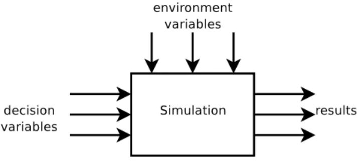
A Parameter Optimization Problem can be defined as having:

• A set of decision variables ~(x) whose values will influence the result of the objective function.

• A set of constraints on the decision variables (gj).

• A set of environment (~y) variables that can not be controlled but influence the result of the simulation.

• An objective function (f(~x, ~y))that needs to be maximized or minimized. The objective function is often a weighted sum of the set of results from the simu-lation (see Section 2.4 for Multiple Response Simusimu-lations).

In Figure 2.1 it can be seen how decision and environment variables interact in a simulation.

Figure 2.1: A Simulation with its intervening variables

Simulation Optimization procedures are used when our objective function can only be evaluated by using computer simulations. This happens because there is not an analytical expression for our objective function, ruling out the possibility of using differentiation methods or even exact calculation of local gradients. Normally these functions are also stochastic in nature, causing even more difficulties to the task

(22)

2.2. Discrete Variables Optimization Algorithms 8

of finding the optimum parameters, as even calculating local gradient estimates becomes complicated.

Running a simulation is always computationally more expensive than evaluating analytical functions thus the performance of optimization algorithms is crucial.

In the following sections, some of the algorithms that have been developed over the years, to solve simulation optimization problems, will be analyzed.

2.2 Discrete Variables Optimization Algorithms

The most simple scenarios in parameter optimization problems happen when de-cision variables are discrete in nature. In these scenarios, and when the subset of possible values for the decision variables is small, one could test every set of values in order to find the optimum solution for the problem. This would be easily accom-plished if the simulation was deterministic. However, as noticed by [Olafsson 02], in the stochastic world, further analysis would have to be done in order to better com-pare each possible solution. [Goldsman 94, Goldsman 98] described several methods to perform this analysis in order to increase the confidence in selecting the optimum result.

The cases that will be analyzed in detail are those where it is infeasible to test every possible solution. The algorithms used in these kind of scenarios are usually called Random Search algorithms (or Meta-Heuristics). [Olafsson 02] noticed that Random Search algorithms usually follow the structure depicted in Algorithm 1.

Random Search algorithms are variations of this algorithm with different neighbour-hood structures, different methods of selecting new candidate solutions and different acceptance and stopping criteria.

In discrete decision variable optimization problems, the neighbouring solutions to a particular set of decision values can be calculated easily, making Random Search

(23)

Algorithm 1 Random Search basic form

1. Select an initial solution and test its performance

2. Select a candidate solution from the neighborhood of that solution and test its performance

3. If the performance of the new solution is better than that of the current solu-tion then set the current solusolu-tion as being the new solusolu-tion

4. If stopping criterion is met stop else go back to step 2

methods ideal for these kind of scenarios.

In the following sections, different Random Search algorithms, that can be found in optimization literature, will be described.

2.2.1 Hill Climbing

Hill Climbing (HC), in its basic form, is the simpler of the optimization methods for discrete variable optimization problems. The method starts with an initial random solution and searches amongst its neighbours for better ones. If a better solution is found the algorithm resumes its search from that new solution. The algorithm stops when it cannot find a better solution close to the current one. A description of a standard HC algorithm can be found in Algorithm 2.

Algorithm 2 Standard Hill Climbing Algorithm

1. Generate an initial solution, randomly or by means of an heuristic function 2. Loop until a stop criterion is met or there are no untested neighbour solutions:

(a) Test a neighbour solution to the current that hasn’t yet been tested (b) If the new solution is better than the current solution make it the current

solution

3. Return the current solution

HC has some well-known limitations as stated by [Russell 02]:

(24)

neigh-2.2. Discrete Variables Optimization Algorithms 10

bours solutions but is not the highest value of the function. The HC algorithm will stop at these points.

• Plateau - A plateau is an area where the objective function is essentially flat. HC will search erratically in these kind of areas.

• Ridges - A ridge is an area with a point, where even without it being a local maximum, all available moves will make the solution worse. Ridges depend on the method chosen to calculate neighbour solutions.

A solution to the Local Maximum problem is to restart the HC process when it stops from a random location. This method, called Random Start Hill Climbing (RSHC), works well when there are only a few local maximums but in more realistic problems it will take an exponential amount of time to find the best solution to the problem ( [Russell 02]).

A variation of the Hill Climbing method is the Steepest Ascent Hill Climbing (SAHC) algorithm ( [Rich 90]). The difference between these two methods is that the first tests all current solution neighbours in order to find the best solution amongst them, while the SAHC algorithm changes its current best solution as soon as a better one is found. SAHC normally converges quicker than HC but still does not guarantee the best solution is found.

Some other methods, loosely based on HC, have been later proposed by other au-thors. In the following sections some of these methods will be analyzed.

2.2.2 Simulated Annealing

Originally described by [Kirkpatrick 83] Simulated Annealing (SA) tries to emulate the way in which a metal cools and freezes into a minimum energy crystalline struc-ture (the annealing process) and compares this process to the search for a minimum in a more general system.

(25)

At that time, it was well known in the field of metallurgy that slowly cooling a material (annealing) could relieve stresses and aid in the formation of a perfect crystal lattice ( [Fleischer 95]). [Kirkpatrick 83] realized the analogy between energy state values and objective function values, creating an algorithm that emulated that process.

The SA algorithm tries to solve the Local Maximum problem described in 2.2.1. It does so by allowing the search to sometimes accept worst solutions with a probability (p), that would diminish with the temperature of the system (t). In this way, the probability of accepting a solution that resulted in a certain increase in the objective function (∆f ), at a certain temperature, would be given by the following formula described in the original paper by [Kirkpatrick 83]:

p(∆f, t) =    e−∆f t ∆f ≤ 0 1 ∆f > 0 (2.1)

Observing the formula, it is clear that downhill transitions are possible, with the probability of them occurring decreasing with the height of the hill and inversely related to the temperature of the system.

In order to implement the SA algorithm, the initial temperature of the system, and how that temperature is going to be lowered, still has to be decided. The slower the temperature is decreased, the greater the chance an optimal solution is found. In fact [Aarts 89] showed that running the simulation an infinite number of times is needed to be sure the optimal solution to the problem has been found.

Most times a reasonably good cooling schedule can be achieved by using an ini-tial temperature (T0), a constant temperature decrement (α) and a fixed number of iterations at each temperature. These kind of cooling schedules are called fixed schedules. The problem with these schedules is that it is often impractical to cal-culate the ideal values for T0 and α. Another approach is to use a scheduling that can automatically adapt to the problem at hand. These are called self-adaptive

(26)

schedules and were first presented by [Huang 86].

2.2.3 Tabu Search

Tabu Search (TS) is another optimization method created to solve the local max-imum problems revealed by the Hill Climbing algorithm. The main idea behind the TS algorithm is to use the search history in order to impose restrictions, and additions, on the neighbourhood of the solution currently being analyzed.

There are two main ways of taking advantage of the search history in order to im-prove the choice of the next solutions to be explored: recency memory and frequency memory ( [Glover 93]).

Recency memory is a short term memory where recent solutions or recent moves between solutions are labeled as being tabu-active. The TS algorithm avoids going through those same solutions, or backtracking those moves, in order to better explore the space of feasible solutions.

Frequency memory is a longer term strategy that discourages moves to solutions whose components have been frequently visited or encourages moves to solutions whose components have rarely been evaluated. Another form of longer term strat-egy is achieved by recording which components appear most in elite solutions and encouraging moves towards solutions containing those components.

Shorter and longer term strategies can be used at the same time and often yield good results. [Glover 93] has written a very comprehensive explanation on the uses of Tabu Search.

2.2.4 Evolutionary Computation

Not uncommonly, computer scientists grab their ideas from biological phenomena. Evolutionary Computation (EC) is just one of many examples of the benefits of this

(27)

Figure 2.2: Mutation and Recombination Operators

interdisciplinary cooperation.

As seen in the last sections, the SA and TS algorithms are variations of the HC algorithm where the notion of neighbourhood has been slightly distorted in order to escape from local maximums. EC has a somewhat different approach as its methods deal with populations of solutions, instead of a single current solution from where moves to better (or sometimes worse) solutions can be made. It is loosely based in the biological mechanism of evolution, where the fittest organisms have a greater probability of generating offspring making each new generation better than the previous one.

Three major methods have been established in literature: Genetic Algorithms (GA), Evolution Strategies (ES) and Evolutionary Programming (EP). These three meth-ods follow, nevertheless, the same basic strategy: A population of solutions, each one of them having a certain fitness (calculated by evaluating the objective func-tion for each solufunc-tion), to whom a series of probabilistic operators, like mutafunc-tions, selections and recombinations, are applied (see Figure 2.2).

The mutation operator is used to introduce innovation in the current population allowing the algorithms to explore areas of the search space that are not being explored at the moment. The selection operators are those that make the method

(28)

reach better results with each new generation, selecting the solutions with an higher fitness value over the ones with a lower one. The recombination operator allows some information exchange between current solutions by introducing a new solution into the population from the merge of two previous selected solutions . The beauty of the algorithm lies in the fact that, although it is extremely simple, it has been used by mother nature, with remarkable success, for millions of years.

Algorithm 3 is a simple outline of what a standard Evolutionary Computation al-gorithm looks like ( [Holland 75, Pierreval 00]).

Algorithm 3 Standard Evolutionary Algorithm 1. Start with the generation counter equal to zero.

2. Initialize a population of individuals (either randomly or by means of an heuris-tic function).

3. Evaluate fitness of all initial individuals in population. 4. Increase the generation counter.

5. Select a subset of the population for children reproduction (selection). 6. Recombine selected parents (recombination).

7. Perturb the mated population stochastically (mutation). 8. Evaluate the mated population’s fitness (evaluation).

9. Test for termination criterion (number of generations, fitness, etc.) and stop or go to step 4.

As has already been stated, the three different approaches to evolutionary computing share the same basic structure. The main differences between them lie in their objectives, the way their population is coded and the way they use the different evolutionary operators.

EP has been initially developed having in mind machine intelligence. Its main particular characteristic is the fact that solutions are represented in a form that is tailored to each problem domain. EP tries to mimic evolution at the level of reproductive populations of species, and recombinations do not occur at this level, so EP algorithms seldom use it.

(29)

On the other hand GAs use a more domain independent representation (normally bit strings). The main problem with GA is how to code each solution into meaningful bit strings. Its advantages are that mutation and recombination operators are easily implemented as bit flips (mutations) and string cuts followed by concatenations (recombination).

The main difference between ES and the other two methods just discussed are the fact that selection in ES is deterministic (the worst N solutions are discarded) and that ES uses recombination as opposed to EP.

A more complete description about the differences between these three methods and their uses can be found at [Spears 93, Fogel 95].

2.2.5 Nested Partitions

The Nested Partitions method is a relatively recent (when compared to other) method for parameter optimization first proposed by [Shi 97, Shi 00]. The basic idea behind this particular method is the continuous partitioning of the solution space into smaller, and more promising, regions until a stopping criterion is met.

The algorithm runs in 4 simple steps: partitioning, sampling, promising index cal-culation and backtracking. The starting step is the creation of an initial, most promising, region (normally the complete solution space Θ). This region is then partitioned into M subregions (σ1, . . . , σM) using some previously chosen partition-ing method. The method then proceeds by randomly samplpartition-ing each one of the M subregions and then calculating the promising index of these subregions as, for in-stance, the best performance value from the samples taken of each subregion. The subregion with the best performance index becomes our most promising subregion and is partitioned even further. In the following steps each of the new subregions and also the surrounding of our most promising region is taken into account, thus calculating the promising index for M+1 regions. If the subregion with the most promising index is one of the subregions of our most promising region, the method

(30)

then continues partitioning even further, but if it is the surrounding region that is se-lected, it backtracks to the region which is the parent to the current most promising region.

Figure 2.3 contains an example of how the algorithm works. In the first step the solution space was partitioned in four subregions. Sub region σ2 was selected as the most promising, after sampling and calculating the promising index of each one of them. The the algorithm proceeded by partitioning region σ2 and evaluating its subregions and also the surrounding region Θ \ σ2 = {σ1, σ3, σ4}. This time subregion σ2.3 was selected as the most promising region. In the next step the promising indexes of our four subregions, plus the surrounding region Θ \ σ2.3, was calculated. As the surrounding region was found to be the most promising, the algorithm backtracked to the parent of subregion σ2.3 which is region σ2.

Figure 2.3: Nested Partition Example

A notable feature of the NP method is that it combines global and local search in a natural way. It is also highly suitable for parallel computer structures ( [Shi 97]).

(31)

2.3. Continuous Variables Scenarios 17

2.3 Continuous Variables Scenarios

Optimization of simulation parameters brings some new challenges when those same parameters are continuous instead of being discrete. In these cases the feasible solu-tions space becomes infinite. Methods for solving optimization problems with con-tinuous input parameters can be classified as either gradient-based or non-gradient-based ( [Swisher 00]). Gradient non-gradient-based methods are the most used ones and three sub-classes of these kind of methods can be identified: Gradient Based Search Methods (GBSM), Response Surface Methods (RSM) and Stochastic Approximation Methods (SAM).

2.3.1 Gradient Based Search Methods

GBSMs work by estimating the objective function gradient (5f) to determine the shape of the function and then employing deterministic mathematical techniques in order to find the maximum of that same function( [Carson 97]). Several dif-ferent methods of estimating the gradient have been developed like: Finite Differ-ences, Likelihood Ratios, Infinitesimal Perturbation Analysis and Frequency Domain Method.

The Finite Differences Method (FD), labeled by [Azadivar 92] as the crudest of all gradient estimation methods, works by calculating partial derivatives for each of the free parameters (−→x = (x1, . . . , xn_{) ∈ M):}

δf δxi =

f (x1, . . . , xi + ∆i, . . . , xn_{) − f(x}1, . . . , xi, . . . , xn)

∆i (2.2)

For a simulation with n free parameters at least n+1 runs of the simulation are needed, and if the simulation response happens to be stochastic in nature then several more runs are needed to obtain a more reliable value for each derivative making this method very inefficient.

(32)

2.3. Continuous Variables Scenarios 18

The Likelihood Ratio Estimation Method (LR) described in [Glynn 90] is a much more efficient method of estimating gradients in stochastic scenarios. However, the LR is not appropriate for every simulation and is not suitable for a generic optimization system.

The Infinitesimal Perturbation Analysis (IPA) method of calculating gradient esti-mates, yields a much more interesting approach for a generic optimization system. The IPA assumes that an infinitesimal perturbation, in an input variable, does not affect the sequence of events but only makes their occurrence times slide smoothly ( [Carson 97]). If this statement holds, then the objective function gradient could be estimated from a single simulation run. However gradients calculated with this method are usually biased and inconsistent.

Frequency Domain Analysis (FDA) is based in the following idea: if an output variable is sensitive to one of the input variables and if that same input variable is oscillated sinusoidally, at different frequencies, over a long simulation run, the output variable should show corresponding oscillations in the response. Those same oscillations can then be analysed using Fourier transforms in order to understand how each input variable influences the output variable of the simulation.

2.3.2 Response Surface Methods

Response Surface Methods (RSM) have the great advantage of requiring fewer simu-lations runs than the other methods described. They work by trying to fit regression models to the objective function of the simulation model. They start by trying to fit a first order regression model into the simulation results and searching that model using a Steepest Ascent approach. When it gets nearer to the solution, a higher order regression model is then used.

Although RSMs require few simulations runs, experiments have shown that for more complex functions the results provided are not very good ( [Azadivar 92]). The usage of regression models in simulation optimization have been described in [Biles 74].

(33)

2.4. Multiple Response Simulations 19

2.3.3 Stochastic Approximation Methods

Stochastic Approximation Methods (SAM) are recursive procedures that approach the maximum of a function also using regression functions. The relevant characteris-tic of this method over RSM is that SAM also work with noisy observations [Azadi-var 92]. The greatest problem is that a large number of iterations is required before reaching the optimum value. For multi-dimensional decision variables, n+1 obser-vations must be done in each iteration.

2.4 Multiple Response Simulations

Simulation models that output more than one result in each simulation run have their own difficulties. With these kind of simulations there is no longer a single objective function that as to be optimized, but several ones.

One simple approach to solve this problem is to consider one of the objective as the function to be optimized subject to certain levels of achievement by the other secondary objective functions [Azadivar 92].

Other obvious solution is to define a weight for each one of the objective functions thus defining a new objective function:

f (~x) = n P i = 1

wifi(~x) (2.3)

This solution, although effective at first glance, is in fact typically a poor solution. Normally each one of the objective functions has a different utility function. By just using the weighted sum of the objective functions, we are considering that these utility functions are linear and have the same zero value but, in fact, the normal case is the one depicted on the right part of Figure 2.4.

(34)

2.5. Non-Parametric Scenarios 20

Figure 2.4: Objective Utility Functions

2.5 Non-Parametric Scenarios

There is also a completely different class of optimization problems. Non-parametric simulations are those where the mathematical models we have seen in Section 2.1 cannot be applied. Examples of these problems are scheduling policies, layout prob-lems and part routing policies [Azadivar 92]. As the decision variables in these problems are not quantitative, classical optimization algorithms like Hill Climbing or Simulated Annealing cannot be used.

To approach this class of problems new model generators and optimization methods had to be developed from scratch. As these problems do not lie in the scope of this thesis no deep analysis will be done about them.

2.6 Conclusions

When having a simulation optimization problem at hand, the first thing one has to do is to analyze the nature of that same problem. This means that decision variables, environmental variables and results must be characterized. The characterization of these variables will automatically narrow the scope of choices one has to make.

In the event of it being a simple discrete variable optimization problem the choice of available algorithms will comprehend the classic Hill Climbing, Simulated Annealing, Tabu Search and several flavours of Evolutionary Computing algorithms, besides the

(35)

2.6. Conclusions 21

more recent Nested Partitions algorithms and also many more. The first three of these algorithms share the same structure having just a few variations. In fact, all of them imply the definition of solution neighbourhoods. One thing they all have in common is the need of evaluating the objective function for comparison purposes. This, as has been seen, brings new challenges when we have several objective functions.

Although having been under heavy research for many years, the studied Simula-tion OptimizaSimula-tion algorithms all fail in one single point. They all assume that the simulation environment is static when in fact it normally is not. The simulation environment is constantly changing and so, the parameters that control it also have to change.

In Chapter 4 some of the optimization algorithms that were just described, as well as clustering methods like the ones that will be analyzed in Chapter 3, will be used in order to develop an optimization system that assumes simulation can be dynamic.

(36)

Chapter 3 Clustering

Clustering can be defined as grouping sets of elements that are similar in some way. A simple way of achieving this objective is by obtaining maximum inter-cluster similarity and intra-cluster dissimilarity.

Clustering methods have to deal with two different problems: membership (whether an element belongs to a certain cluster or not) and how many clusters to create. Most methods only deal with the first of these problems but some strategies have been developed to determine the number of clusters and cluster membership at the same time ( [Fraley 98]).

To develop an optimization system as delineated in Chapter 1, solutions from an optimization problem must be grouped together, having in mind that different solu-tions apply to different initial condisolu-tions of the simulation. The objective is to find out which different kind of solutions exist and to which type of problems each one of them can be applied.

In this section, different clustering algorithms will be explained. The situations in which each algorithm can be used, their advantages and drawbacks will also be analyzed.

(37)

3.1. Clustering Methodology 23

3.1 Clustering Methodology

Clustering is normally done in 5 separate steps ( [Jain 99]):

1. Pattern Representation - This refers to preparing the data for the cluster-ing algorithm. Analyzcluster-ing which data elements are relevant to the clustercluster-ing process, their scales and types, and also transforming the data in order to emphasize more relevant features (e.g. transforming numbers into even and odd classes).

2. Definition of Pattern Proximity - Clustering is normally based in some kind of proximity function. This function can be simply the euclidean distance between each element or a somewhat more complex function.

3. Clustering - There are many methods for performing this step and those can be grouped, for example, as hard or fuzzy partitioning methods and hierarchi-cal or partitioning methods.

4. Data Abstraction - How the data will be presented after the clustering step.

5. Assessment of Output - Validating the clustering process output.

A vast number of clustering algorithms exist due to the fact that each specific clustering problem has its own requirements and benefits. However, an all-solving clustering algorithm is something that does not exist [Jain 99].

3.2 Patterns and Features

Patterns ( ~p) are a common clustering term that refer to vectors of d measurements. Patterns are the data items that a clustering algorithm will try to group. Each scalar component of a pattern is called a feature (pi).

(38)

3.3. Clustering Techniques Classification 24

~

p = (p1, . . . , pd) (3.1)

Features can be divided into the following categories ( [Gowda 91]):

• Quantitative Features: continuous values, discrete values or interval values; • Qualitative Features: nominal (unordered) or ordered.

To cluster the data retrieved from the optimization model described in Chapter 1, focus will be given mainly to clustering methods appropriated for continuous or discrete values.

3.3 Clustering Techniques Classification

As stated before clustering techniques can be classified from several different point of views. Classifying these algorithms can help in the choice of a suitable clustering algorithm. Following, we present a classification of clustering algorithms based on the one proposed by [Jain 99]:

• Agglomerative / Divisive - Agglomerative methods start with each pattern in its own cluster and work by merging clusters until a stopping criterion is met. Divisive methods start with a single cluster containing all patterns and work by dividing the initial cluster into smaller clusters, also until a stopping criterion is met. Agglomerative methods memory requirements are usually proportional to the square of the number of groups in the initial partition, normally the size of the data set [Fraley 98].

• Monothetic / Polythetic - Most clustering methods use all features at once when computing distances between patterns. These kind of methods are referred as polythetic methods. Monothetic methods considers features sequentially as they divide or agglomerate clusters.

(39)

3.4. Cluster Distance Heuristics 25

• Hard / Fuzzy - Clustering algorithms can have hard or fuzzy result sets. In hard result sets each pattern belongs to only one cluster while in fuzzy result sets each pattern is assigned a degree of membership to more than one cluster.

• Incremental / Non-incremental - Incremental clustering algorithms allow the introduction of new patterns into the result set without forcing a complete rebuild of the pattern set. This is of extreme importance when the pattern set is large and dynamic.

• Hierarchical / Partitioning - Hierarchical clustering algorithms can output a dendogram of nested clusters as a result, while partitioning algorithms output single-level partitions.

3.4 Cluster Distance Heuristics

Most of the clustering methods we will discuss use some heuristic form of determin-ing the distance between clusters. In fact, the existdetermin-ing methods normally concen-trate their efforts in determining the dissimilarity between clusters rather than their similarity.

The most appropriate heuristic to be applied is something that depends strongly on the dataset, so a best than all method is something that does not exist. Besides that, a criteria to find which method is the best for a certain dataset is not known. The most used heuristic variations are the following ( [Fung 01]):

• Average linkage - In this method dissimilarity is calculated as the average distance between each element in a cluster and all elements of the other cluster.

• Centroid linkage - The centroid of a cluster is defined as the center of a cloud of points. Dissimilarity is calculated as the the distance between cluster centroids.

(40)

3.4. Cluster Distance Heuristics 26

• Complete linkage - The distance between two clusters is determined by the distance between the most dissimilar elements of both clusters. This method is also referenced as the furthest-neighbour method.

• Single linkage - This method is a variation of the previous one where the dissimilarity between two clusters is based on the two most similar elements instead of the two most dissimilar ones.

• Ward’s method - A somewhat different method from the previous ones. Cluster membership is assigned by calculating the total sum of squared devi-ations from the mean of the cluster.

Another problem regarding distances is that the various features normally do not use the same scale. Normalization has to be performed in order to get meaningful distance values.

[Luke 02] defined a method that ensures all features will have a mean value of 0.0 and a standard deviation of 1.0 over the entire range of patterns to be analyzed. His method can be easily explained using these four simple steps to be applied to each feature:

1. Sum the values of the feature over all patterns and divide the sum by the number of different patterns.

2. Subtract this average value from the feature in all patterns.

3. Sum the square of these new values over all patterns, divide the sum by the total number of patterns, and take its square-root. This is the standard devi-ation of the new values.

4. Divide the feature by the standard deviation in each pattern.

Only after applying this simple procedure will all patterns be ready for comparison and distance evaluation.

(41)

3.5. Initial Clustering Centers 27

3.5 Initial Clustering Centers

Some of the methods we are describing in the next section require a set of initial empty clusters and their respective centers. The choice of these initial centers is crucial to the quality of the obtained clusters, as noticed by [Fung 01]. The same author proposed some heuristic methods for choosing these initial parameters:

• Bins - Divide the space into bins and choose random initial clusters in each of those bins.

• Centroid - Choose initial centers near to the dataset centroid. • Spread - Chose random centers across the entire dataset.

• PCA - Project the dataset into the most important component as to form a one-dimensional dataset. Then perform a clustering algorithm and use the obtained clusters centers as the initial centers.

3.6 Clustering Methods

In the next sections several clustering methods described in the literature will be presented.

3.6.1 K-Means

The K-Means clustering algorithm was one of the first clustering algorithms ever described. Although very easy to implement, it has some drawbacks that will be discussed later in this Section.

The algorithm starts with the creation of k clusters with initial centroids estimated using, for example, one of the algorithms explained in Section 3.5. Patterns are then assigned to the cluster with the nearest centroid (usually using simple euclidean

(42)

3.6. Clustering Methods 28

distance measurements). New cluster centroids are then calculated and the process repeats until convergence is met (i.e. no pattern changes cluster).

The major drawbacks of this method are: the fact that the number of clusters must be predetermined; having a poor performance as distances to the cluster centroids must always be recalculated in each step; and its results being very dependent of the initial choice of cluster centroids.

[Fayyad 98] showed that the dependency of the initial clusters choice could be easily surmounted by iteratively applying the K-Means algorithms to various subsamples of the initial set of patterns and observing which initial clusters fail to have any elements in it. Other problem with this method is that it favours circular clusters (as most clustering methods do), however clusters can have different forms like, for example, strips or ellipsoids.

3.6.2 C-Means Fuzzy

Fuzziness is a term often used in artificial intelligence literature that breaks the traditional approach of an object x having, or not having, a certain characteristic y. Instead of that, fuzzy methods state that the object x has the characteristic y to a certain degree z. This approach is able to represent reality in a much accurate form.

When it comes to clustering, fuzziness means that patterns no longer belong un-doubtedly to a single cluster but have a certain degree of membership to a number of different clusters. This creates the notion of fuzzy boundaries. The C-Means Fuzzy algorithm, first described by [Pal 95], works like depicted in Algorithm 4.

The C-Means algorithm usually has a parameter q (a real number greater than 1) that refers to the amount of fuzziness applied to the cluster boundaries. The degree of membership to each cluster (uij) is computed using the following formula:

(43)

Algorithm 4 C-Means Fuzzy Clustering Algorithm

1. Estimate K initial empty clusters with estimated centroids (using a method like those exposed in Section 3.5).

2. Calculate the degree of membership of every pattern to every cluster. 3. Recalculate cluster centroids.

4. Update the degree of membership (same as step 2).

5. Go to step 3 unless a stopping criterion is met (usually when the biggest change in membership is below a certain tolerance value).

uij = 1 d(pj,Ci) 1 q−1 PK k=1 d(pj1,Ck) 1 q−1 (3.2)

Where the pj refers to pattern j, Ci refers to cluster i and d is a distance estimator as defined in Section 3.4.

To update the cluster centroids we just have to take into account the degree of membership of each of the M patterns to each cluster:

˙ Ci = PM j=1(uij)qpj PM j=1(uij)q (3.3)

The objective of the algorithm is to minimize the following cost function:

E(U, C) = M X j=1 K X i=1 (uij)q_d(pj_{, Ci)} _(3.4)

3.6.3 Deterministic Annealing

The deterministic approach to clustering, first introduced by [Rose 90], follows much of the principles of the SA algorithm described in Section 2.2.2. In this case the energy of the system, that we want to minimize, is given by the following expression (extremely similar to the cost function seen in equation 3.4):

(44)

3.6. Clustering Methods 30 E = M X j=1 K X i=1 (uij)d(pj, Ci) (3.5)

In the original paper, the problem is formulated as a fuzzy clustering problem and the association probability distribution is obtained by maximizing the entropy at a given average variance .

3.6.4 Clique Graphs

The recent popularity of clustering in the domain of bio-informatics, as a tool for studying DNA micro-array data, has yield some interesting new results [Fasulo 99].

One of the most interesting results being a new clustering algorithm based on clique graphs, or, more precisely, on corrupted clique graphs. Clique graphs are graphs with every vertex connected to every other vertex.

The algorithm, first described by [Ben-Dor 99], tries to maximize intra-cluster sim-ilarity and inter-cluster dissimsim-ilarity. In this way the simsim-ilarity graph, within a cluster, should be represented by a clique graph.

However the similarity measurements are usually approximations and errors are prone to occur. So similarity is normally represented by a clique graph with some edges missing and some extra edges. This kind of graphs are what are called cor-rupted clique graphs.

In the corrupted clique graph model it is assumed that the similarity graph is a clique graph with edges removed and added with a probability α. The goal of the algorithm is to find the ideal clique graph given the corrupted one [Fasulo 99].

The theory behind the algorithm states that if α is not to large and M is not to small, meaning that we have a sufficiently large number of patterns, and similarity errors are not to big, then, we can choose a subset of the initial patterns p0 _with high probability of it containing a core that correctly classifies all patterns in the

(45)

Algorithm 5 Corrupted Clique Graph Clustering Algorithm 1. Pick a random subset p0 _{of p.}

2. Consider all ways of partitioning p0 _{into non-empty clusters (core candidates).} 3. Classify all remaining patterns into these candidates.

4. Keep the core candidate with the clique graph more similar to the original clique graph.

initial dataset. The theoretical algorithm base on this assumption is described in Algorithm 5.

3.6.5 Hierarchical Clustering

Hierarchical Clustering is a common class of clustering algorithms, suitable for sce-narios where there is not a obvious separation by well-defined clusters. Instead, these algorithms, output clusters that are represented as a tree where the root node is a cluster containing all patterns and sub-sequential nodes are divisions of that node.

Hierarchical clustering methods come in two flavours: divisive and agglomerative. The first start with a big cluster containing all patterns and work down the tree by breaking it into smaller ones, while the latest start with small uni-pattern clusters that are joined, creating increasingly larger clusters. Agglomerative hierarchical clustering algorithms are much more common and are the ones that will be described next.

The idea behind the algorithm is to start by creating a cluster for each pattern in the dataset, then, find out which pair of clusters is less costly to merge, and merge it. The merging process then repeats until there is only one cluster left (see Figure 3.1). To estimate the cost to merge two clusters any of the methods described in Section 3.4 can be used.

(46)

Figure 3.1: Hierarchical Clustering

a certain number of clusters as been achieved or when the merging cost crosses a determined tolerance value (see Figure 3.1 - stopping at dashed line creates the clusters with a thicker border in the image).

3.6.6 Local Search

The same optimization techniques studied in Section 2.2 can be easily adapted to provide clustering algorithms. The main idea behind this technique is to look at a cluster configuration as a solution for the clustering problem. This solution can then be optimized using, for instance, the SA algorithm. In this case, swapping patterns from a cluster to another could be used to create neighbouring solutions.

An even better utilization of optimization techniques can be achieved if, instead of creating an initial random solution, we apply a simple clustering algorithm (i.e. k-means) prior to trying any optimization.

[Kanungo 02] has a good overview of various swap strategies that can be applied to local search methods in order to improve the k-means method.

(47)

3.7. Conclusions 33

3.6.7 Dynamic Local Search

Recently a new clustering method was developed, called Dynamic Local Search ( [Karkkainen 02]), that claims to be able to solve, simultaneously, the two main questions clustering algorithms try to answer: how many clusters exist and to which cluster each pattern belongs to.

The original idea behind the method is that Local Search can be used, in a brute force manner, to generalize the problem to one where we do not know the number of existing clusters. This is done by applying the method to every reasonable number of clusters and choosing the one that minimizes the cost function. This method has the obvious drawback of being terribly inefficient.

[Karkkainen 02] rationalized that it was possible to use the Local Search method-ology to solve both problems at the same time simply by adding the removal and creation of clusters to the operations that generate neighbouring solutions.

3.7 Conclusions

In this Chapter several clustering algorithms have been addressed. The clustering problem and its variants have also been explained and listed.

Clustering is a much harder problem than what can be supposed at first glance. The vast number of different clustering algorithms that can be found in literature is a reflex of the great number of different problems, with each one requiring different approaches.

Besides having to choose from a great variety of algorithms, several small details have to be decided when applying clustering techniques like how to calculate distances between elements and clusters. There is also a major problem found with every clustering algorithm: without any sense of scale it is impossible to assign elements to clusters without any user input.

(48)

3.7. Conclusions 34

In Chapter 4 some of the clustering algorithms that were just presented, as well as optimization methods like the ones that were analyzed in Chapter 2, will be used in order to develop a optimization system like the one presented in Chapter 1.

(49)

Chapter 4 Project and Implementation

A generic optimization system has been implemented to validate the ideas behind this dissertation. Four main points are behind the construction of this prototype:

• In the simulation optimization field, researchers often develop their own opti-mization systems. This happens mainly because it is relatively easy to develop a fairly decent optimizer from scratch. However having a generic optimization system available would allow the researcher to optimize his simulation with several, and perhaps more advanced, optimization methods and use some al-ready developed analysis tools.

• No system is ever generic enough for everyone. So, having the possibility of extending a system is crucial when developing a generic system. In particular this optimization system should allow new optimization methods to be added easily.

• Simulation based optimizations are always, or almost always, CPU intensive. This happens because optimization algorithms need to run simulations, which sometimes are already CPU intensive, numerous times, in order to achieve good results. An usable optimization system must take this into account. Distribution is the most obvious way of working around this problem, so a

(50)

4.1. Architecture 36

good optimization system should allow the distribution of workload across different machines.

• Simulations are used many times to optimize a set of parameters that will be later used in the real world. Most optimization systems approaches do not take into account the fact that there are environment changes occurring every time in real life applications.

• A much needed feature in todays optimization systems, that will help un-derstand and cope with changing environments, would be a scenario/result analyzer. This tool would help users understand what kind of solutions there are to the problem and in which scenario each can be applied successfully.

The next sections will explain how a system based in this previous ideas could be, and was, developed.

4.1 Architecture

As already explained in Chapter 2, a simulation normally receives a set of parameters and outputs a set of results. Besides that, most simulations have a set of environment parameters that can be user adjusted or randomly selected.

A generic optimization system must to cover as many different configurations as possible. However, creating a system that is to complicated to use should be avoided. So, a few concessions had to be made in order to keep the system simple. However, the system should allow different simulation configurations to be used by means of system extensibility.

The system will be composed of several modules that will be introduced in the following paragraphs and explained in full detail in the subsequent sections.

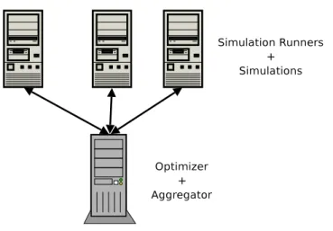
To begin, a module that will interact with the different type of simulations will be needed. This module should, first of all, be distributable so we can have several

(51)

4.1. Architecture 37

Figure 4.1: Master-Slave Architecture

instances of it running in different machines (see Figure 4.1). It should also be able to receive a binary file for a certain simulation, instructions on how to run it with different parameters and how to gather results from it.

A second module, that will work closely with the one just described, will be respon-sible for evaluating simulation runs. Another task of this module will be to mask the fact that simulations are normally stochastic in nature.

Optimization is obviously the major goal of the system so an optimization module is essential. This module will use the evaluator module in order to get the results from various simulation runs and use these results to find the optimum parameters for a given scenario.

A final module will aggregate and analyze results from the optimizer, in order to create a dynamic optimization schedule for the simulation, and allow the user to better understand how parameters and scenarios influence each others. The aggre-gator module will talk to the optimizer as well as with the evaluator. Figure 4.2 captures the various modules and their interaction.

(52)

4.2. Technology 38

Figure 4.2: System Modules Interaction

4.2 Technology

The most important choices made when deciding the technology to be used in the project, were selecting the programming language and the communication proto-cols to be used. The choice was the Java programming language because of its multi-platform characteristics, as it would make it easier to find a large set of com-puters available for hosting simulation runners, and the XML-RPC communication protocol for its excellent Java implementation, easiness of use and multi-platform characteristics.

4.3 Modules

In the next sections we will take a more detailed look into the inner workings of each of the modules that compose the optimization system.

4.3.1 Simulation Runners

Simulation Runners are responsible for the interaction between the optimization system and the simulations being optimized. Three particular aspects have to be dealt with:

(53)

4.3. Modules 39

• Simulation version awareness and differentiation; • Communication with the optimization system; • Interaction with a diversity of simulations.

Simulation runners have to be able to differentiate between simulation projects and even between versions from the same project. One solution could be to send the project code every time a simulation run was demanded from a simulation runner. This solution has obviously a great drawback, as sometimes the simulation code can be quite large and time would be wasted in communications.

The solution found to this problem was a simple one. Every time the server starts working on a new project it calculates a fingerprint for that specific project. The fingerprint is calculated simply by means of a MD5 hash function applied to the name of the simulation file and its size in bytes. This solutions assumes that two different projects with the same filename and the same file size are very uncommon.

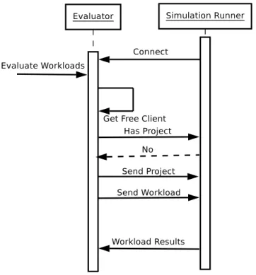
To allow the simulation runners to receive orders from the optimization system a simple communication protocol had to be developed. The protocol consists of three simple messages:

• hasProject(String hash) - This method will allow the optimizer to query the simulation runners if they already have the code for a certain project, thus preventing unnecessary communications. The single parameter of this function is the hash code of the project.

• createProject(String hash, String filename, byte[] contents) - If the simulation runner does not have the code for the project the optimizer will then issue a request for the project creation. The parameters for this request will be the hash code of the project, the filename where the project code has to be stored and the contents of the project themselves.

• receiveWorkloadRequest(String hash, String commandline, Vector params, Vec-tor values) - After the simulation runner receives the code of the project the

(54)

4.3. Modules 40

Figure 4.3: Simulation Communication

optimizers can start issuing requests for the execution of workloads. Besides sending the hash of the project to be executed, the optimizer will also send the command line that the simulation runner should use and two vectors con-taining the parameters for this concrete execution and their respective values.

Simulation runners would also have to communicate the results of the simulations back to the optimizer system. This communication will be detailed in the following section.

Another situation that had to be dealt with the simulation runners was how to com-municate the different parameter values to diverse simulations. Each simulation will, of course, expect to receive their parameters in a different form. As it is impossible to imagine all the forms of interfacing with different simulations we resorted to the possibility of extension.

An abstract class (see Figure 4.3) was created with a single method: communi-cateParameters. This method would receive the parameters, and their respective values, that are to be communicated to the simulation. The several implementa-tions of this class could then write to the correct files, and in the correct form, the values to be passed to the simulation. The possibility of this method chang-ing the command line, in order to communicate the values by that mean, was also contemplated by adding a return value.

For testing purposes, a simulation communicator capable of writing to property files (a common file type used in the Java language) was implemented.

Dynamic scenario simulation optimization

Dynamic Scenario Simulation Optimization

A Thesis presented for the degree of

Master in Artificial Intelligence and Intelligent Systems

Universidade do Porto

Faculdade de Engenharia

Dedicated to

Dynamic Scenario Simulation Optimization

Submitted for the degree of Master in Artificial Intelligence and

Intelligent Systems

June 2006

Abstract

Optimiza¸

c˜

ao de Simula¸

c˜

oes em Cen´

arios

Dinˆ

amicos

Submetido para obten¸c˜ao do grau de

Mestrado em Inteligˆencia Artificial e Sistemas Inteligentes

Junho de 2006

Resumo

Acknowledgements

Contents

List of Figures

List of Tables

List of Algorithms

Listings

Chapter 1

Introduction

1.1

Objectives

1.2

Proposal

1.3

Thesis Structure

Chapter 2

Simulation Optimization

2.1

Parameter Optimization

2.2

Discrete Variables Optimization Algorithms

2.2.1

Hill Climbing

2.2.2

Simulated Annealing

2.2.3

Tabu Search

2.2.4

Evolutionary Computation

2.2.5

Nested Partitions

2.3

Continuous Variables Scenarios

2.3.1

Gradient Based Search Methods

2.3.2

Response Surface Methods

2.3.3

Stochastic Approximation Methods

2.4

Multiple Response Simulations

2.5

Non-Parametric Scenarios

2.6

Conclusions

Chapter 3

Clustering

3.1

Clustering Methodology

3.2

Patterns and Features

3.3

Clustering Techniques Classification

3.4

Cluster Distance Heuristics

3.5

Initial Clustering Centers