Prediction of extreme floods based on CMIP5 climate models: a case study in the Beijiang River basin, South China

(1)

HESSD

11, 9643–9669, 2014

Prediction of extreme floods based on

CMIP5 climate models

C. H. Wu et al.

Title Page

Abstract Introduction

Conclusions References

Tables Figures

◭ ◮

Back Close

Full Screen / Esc

Printer-friendly Version Interactive Discussion

Discussion

P

a

per

|

Discus

sion

P

a

per

|

Discussion

P

a

per

|

Discussion

P

a

per

|

Hydrol. Earth Syst. Sci. Discuss., 11, 9643–9669, 2014 www.hydrol-earth-syst-sci-discuss.net/11/9643/2014/ doi:10.5194/hessd-11-9643-2014

This discussion paper is/has been under review for the journal Hydrology and Earth System Sciences (HESS). Please refer to the corresponding final paper in HESS if available.

Prediction of extreme floods based on

CMIP5 climate models: a case study in the

Beijiang River basin, South China

C. H. Wu1, G. R. Huang1,2, and H. J. Yu1

1

School of Civil Engineering and Transportation, South China University of Technology, Guangzhou 510640, China

2

State Key Laboratory of Subtropical Building Science, South China University of Technology, Guangzhou 510640, China

Received: 4 August 2014 – Accepted: 6 August 2014 – Published: 13 August 2014

Correspondence to: G. R. Huang ([email protected])

(2)

HESSD

11, 9643–9669, 2014

C. H. Wu et al.

Title Page

Tables Figures

◭ ◮

Back Close

Full Screen / Esc

Discussion

P

a

per

|

Discus

sion

P

a

per

|

Discussion

P

a

per

|

Discussion

P

a

per

|

Abstract

The occurrence of climate warming is unequivocal, and is expected to be experienced through increases in the magnitude and frequency of extreme events, including flood-ing. This paper presents an analysis of the implications of climate change on the future flood hazard in the Beijiang River basin in South China, using a Variable Infiltration Ca-5

pacity (VIC) model. Uncertainty is considered by employing five Global Climate Models (GCMs), three emission scenarios (RCP2.6, RCP4.5, and RCP8.5), ten downscaling simulations for each emission scenario, and two stages of future periods (2020–2050, 2050–2080). Credibility of the projected changes in floods is described using an uncer-tainty expression approach, as recommended by the Fifth Assessment Report (AR5) 10

of the Intergovernmental Panel on Climate Change (IPCC). The results suggest that the VIC model shows a good performance in simulating extreme floods, with a daily

runoffNash and Sutcliffe efficiency coefficient (NSE) of 0.91. The GCMs and emission

scenarios are a large source of uncertainty in predictions of future floods over the study region, although the overall uncertainty range for changes in historical extreme precipi-15

tation and flood magnitudes are well represented by the five GCMs. During the periods 2020–2050 and 2050–2080, annual maximum 1-day discharges (AMX1d) and annual maximum 7-day flood volumes (AMX7fv) are projected to show very similar trends, with the largest possibility of increasing trends occurring under the RCP2.6 scenario, and the smallest possibility of increasing trends under the RCP4.5 scenario. The projected 20

ranges of AMX1d and AMX7fv show relatively large variability under different future

(3)

HESSD

11, 9643–9669, 2014

C. H. Wu et al.

Title Page

Tables Figures

◭ ◮

Back Close

Full Screen / Esc

Discussion

P

a

per

|

Discus

sion

P

a

per

|

Discussion

P

a

per

|

Discussion

P

a

per

|

1 Introduction

Recent research indicates that extreme precipitation is very likely (greater than 90 % probability) to become more intense and more frequent over most of the mid-latitude land masses and wet tropical regions (IPCC, 2013). Increases in extreme precipitation are expected to trigger floods, and the associated impacts will exceed those of eco-5

nomic damage and cause loss of life. It is therefore extremely important to gain an understanding of the projected changes in extreme flood events under climate change. The most useful tool for investigating the impacts of climate change on floods is a hydrological model driven by outputs from global climate models (GCMs). GCMs are considered to be the most essential and feasible tools for use in supplying useful 10

climate information on global or large scales. However, GCMs generate outputs at a relatively coarse grid scale (of a few hundred kilometres), and therefore their outputs cannot be directly used in climate impact studies at a catchment scale (Sachindra et al., 2014a). Downscaling techniques (e.g., dynamical downscaling and statistical down-scaling) are therefore normally used to link coarse resolution GCM outputs with catch-15

ment scale climatic variables (Sachindra et al., 2014b). Dynamical downscaling is per-formed through regional climate models (RCMs) or limited-area models (LAMs) (Fowler et al., 2007), whereas statistical downscaling defines the empirical relationships be-tween large-scale variable fields (e.g., climate model outputs) and local-scale surface conditions, and translates large-scale GCM outputs onto a finer resolution (Fowler et 20

al., 2007; Tisseuil et al., 2010). Because of the lower computational requirement of statistical downscaling in comparison with those required of dynamical downscaling, it has been widely used in climate impact related research work (Sachindra et al., 2014a, b; Tisseuil et al., 2010). However, despite the increase in resolution, downscal-ing simulation results (e.g. RCM) often remain too biased to be used directly in impact 25

(4)

HESSD

11, 9643–9669, 2014

C. H. Wu et al.

Title Page

Tables Figures

◭ ◮

Back Close

Full Screen / Esc

Discussion

P

a

per

|

Discus

sion

P

a

per

|

Discussion

P

a

per

|

Discussion

P

a

per

|

cumulative distribution functions of observations and model simulations have been de-veloped to produce corrected GCM/RCM simulations (e.g. Bennett et al., 2014; Li et al., 2010). Based on the data provided by GCMs, numerous studies have investigated

the effects of climate change on regional floods over the world, including in Europe

(Feyen et al., 2012), Germany (Huang et al., 2013), Bangladesh (Mirza et al., 2003), 5

Britain (Kay and Jones, 2012), and China (e.g. Liu et al., 2013; Wu et al., 2014; Xiao et al., 2013; and Xu et al., 2013).

In southern China, there is a proven increase in the frequency of flood occurrence since the 1980s, particularly in the Beijiang River basin, a northeastern tributary of the Zhujiang River (Wu et al., 2013b). To our knowledge, only two studies have previously 10

investigated the e_ffects of climate change on extreme floods over the Beijiang River

basin (Wu et al., 2014; Xiao et al., 2013). Furthermore, a large uncertainty is apparent in the projected values of these studies. It is well known that a multitude of sources of uncertainty are involved in analysis of the impact of climate change, including GCM structure, downscaling from GCMs, emission scenarios, and the hydrological models 15

used and their parameters (Chen et al., 2011; Kay et al., 2009; Liu et al., 2013). Among these, GCM structure uncertainty is likely to be the largest source of uncertainty in relation to the hydrological impacts of climate change (Kay et al., 2009; Prudhomme and Davies, 2009). It is therefore necessary to perform additional comparative analyses on the prediction of future floods over the Beijiang River basin to lower the uncertainty 20

of future climate projections.

As a case study, we use a typical high-risk flooding area of the Beijiang River basin, and aim to explore the response of floods to climate change as derived from the CMIP5 climate models, using a large-scale semi-distributed hydrological model. However, this

study differs from previous studies, as it focuses on a comparison of the different GCMs

25

and di_fferent climate change scenarios using di_fferent stages of the future period. In

(5)

HESSD

11, 9643–9669, 2014

C. H. Wu et al.

Title Page

Tables Figures

◭ ◮

Back Close

Full Screen / Esc

Discussion

P

a

per

|

Discus

sion

P

a

per

|

Discussion

P

a

per

|

Discussion

P

a

per

|

2 Data and methodology 2.1 Study area

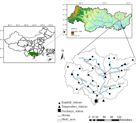
The study area called the Feilaixia catchment is located in the upstream of the Beijiang

River (Fig. 1). It has a drainage area of 34 097 km2and accounts for 73 % of the

Bei-jiang River basin. The Feilaixia catchmen consists of four main tributaries, the WuBei-jiang 5

River, Zhenjiang River, Lianjiang River and Wengjiang River (Fig. 1). The region is an important water source for the Guangdong province, one of the most developed areas of China. The climate of the region is warm wet tropical to subtropical, and precipita-tion during the flood season (April to September) accounts for 70–80 % of the annual precipitation. Location of hydro-meteorological stations used in the study is shown in 10

Fig. 1.

2.2 Datasets

Data used in this study include digital elevation model (DEM), vegetation cover, soil properties, and observed hydro-meteorological data. The DEM (at a resolution of 90 m) was derived from the International Scientific & Technical Data Mirror Site, Com-15

puter Network Information Center, Chinese Academy of Sciences. Vegetation cover-age datasets were collected from the University of Maryland (UMD), and provide in-formation on global land classification at a 1 km resolution (Hansen et al., 2000). The classification of soil texture at a resolution of 1 km based on the Harmonized World Soil Database (HWSD) was provided by the Food and Agriculture Organization of 20

the United Nations (FAO) and the International Institute for Applied Systems Analy-sis (IIASA).

Daily hydrological data as recorded at 27 rainfall stations and 1 discharge station were provided by the Hydrology Bureau of the Guangdong Province, China. Daily max-imum and minmax-imum temperature data from 4 stations were provided by Meteorological 25

(6)

Me-HESSD

11, 9643–9669, 2014

C. H. Wu et al.

Title Page

Tables Figures

◭ ◮

Back Close

Full Screen / Esc

Discussion

P

a

per

|

Discus

sion

P

a

per

|

Discussion

P

a

per

|

Discussion

P

a

per

|

teorological Administration (http://cdc.cma.gov.cn/home.do). The data sets from all the stations spanned over the period from 1969 to 2011.

2.3 CMIP5 climate models

CMIP5 is the Coupled Model Intercomparison Project Phase 5, which provides a frame-work for coordinated climate change experiments for the next several years, and thus 5

includes simulations for assessment in the AR5, as well as for others that extend be-yond the AR5 (Taylor et al., 2012). Relative to earlier phases, CMIP5 focuses on a set of experiments that include higher spatial resolution models, improved model physics, and a richer set of output fields (Gulizia and Camilloni, 2014; Taylor et al., 2012). Addi-tionally, the CMIP5 climate change projections are driven by new climate scenarios that 10

use a time series of emissions and concentrations from the representative concentra-tion pathways (RCPs) described in Moss et al. (2010). Accordingly, GCMs provided by the CMIP5 have been widely used in the assessment of climate change (Gulizia and Camilloni, 2014; Pierce et al., 2013; Smith et al., 2013).

When using multiple GCMs to assess future climate change, the underlying assump-15

tion is that different models provide statistically independent information. In fact, models

usually share physical parameterization schemes, and at times, even large parts of the same code (Pincus et al., 2008), which could lead to similar weaknesses among the models. Pennell and Reichler (2011) evaluated 24 state-of-the-art models of the CMIP3 and their ability to simulate broad aspects of twentieth-century climate, and found that 20

the e_ffective number of models (the amount of statistically independent information

in the simulations) was significantly less than the actual number of models. Xiao et al. (2013) applied the Hierarchical Cluster Analysis (HCA) to analyse the precipitation simulation similarity of 47 CMIP5 GCMs over the Zhujiang River basin, and suggested that the 47 GCMs can be classified into five types.

25

(7)

HESSD

11, 9643–9669, 2014

C. H. Wu et al.

Title Page

Tables Figures

◭ ◮

Back Close

Full Screen / Esc

Discussion

P

a

per

|

Discus

sion

P

a

per

|

Discussion

P

a

per

|

Discussion

P

a

per

|

basin, were used in this study. The GCMs data (precipitation and temperature) used include: (1) an historical simulation for the period 1970–2000 and (2) three new

sce-narios (RCP2.6, RCP4.5, and RCP8.5) for two different future periods (2020–2050 and

2050–2080). The model data and observations used in the study were interpolated to

the same resolution on a 0.25◦

×0.25◦ grid of the study area using bilinear

interpola-5

tion. To reduce system errors in GCM simulations, the bias between the monthly pre-cipitation and temperature of the observed and GCM output data was corrected using a quantile-based mapping method (Li et al., 2010). A stochastic weather generation method was then employed to temporally disaggregate the monthly downscaled cli-mate projections into the daily weather forcings required by the hydrological model. To 10

consider the range of variability that this randomness could induce, multiple

downscal-ing simulations were performed for each projection (Raffet al., 2009). The simulation

set size of this study was arbitrarily set to ten simulations.

2.4 Methodology

Variable Infiltration Capacity (VIC) model developed by Liang et al. (1994) is a macro-15

scale physical hydrological model based on a spatial distribution grid. It can simu-late the physical exchange of water and energy among the soil, vegetation, and at-mosphere in a surface vegetation-atmospheric transfer scheme (Wang et al., 2012). Further detailed information relating to the VIC can be obtained from University of Washington’s website (http://www.hydro.washington.edu/Lettenmaier/Models/VIC/ 20

SourceCode/Download.shtml). As a typical land surface hydrological model, the VIC model has been successfully applied to assess the impact of climate change on hy-drology over the Zhujiang River basin (Wu et al., 2014; Xiao et al., 2013). In this study, the model VIC 4.1.2b is used to simulate only the water balance, and is run over a

regional domain consisting of 69 grid points at a spatial resolution of 0.25◦

×0.25◦.

25

(8)

statis-HESSD

11, 9643–9669, 2014

C. H. Wu et al.

Title Page

Tables Figures

◭ ◮

Back Close

Full Screen / Esc

Discussion

P

a

per

|

Discus

sion

P

a

per

|

Discussion

P

a

per

|

Discussion

P

a

per

|

tical significance of trends in future streamflow series as projected by GCMs. Here, two styles of trends tested are considered: trends tested without considering a level of significance and statistically significant trends at the 0.1 level.

The qualifier of “likelihood”, which provides calibrated language for describing quan-tified uncertainty, can be used to express a probabilistic estimate of the occurrence of 5

a single event or of an outcome (IPCC, 2013). In this study, a total of 50 simulations for each projection of five GCMs were considered as a whole, and then likelihood terms associated with outcomes were defined as (IPCC, 2013):

Very likely: 90–100 %; Likely: 66–90 %; More likely than not: 50–66 %; About as likely as not: 33–50 %; Unlikely: 10–33 %; Very unlikely: 0–10 %.

10

We also use the qualifier “very likely” when, for example, the percentage of samples for one emission scenario shows increasing or decreasing trends of up to 90 %, we conclude that this trend (either increasing or decreasing) is “very likely” to occur.

3 Results and analysis 3.1 VIC model validation

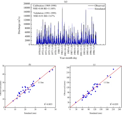
15

Observed forcing data required by VIC model were generated based on 27 rainfall sta-tions with daily precipitation data, and 4 temperature stasta-tions with daily maximum and minimum temperatures data. The recorded data series was divided into two periods: the period 1969–1990 for model calibration and the period 1991–1999 for model

val-idation. The efficacy of the simulation results was evaluated using the Nash–Sutcliffe

20

efficiency coefficient (NSE) and relative error (RE).

As shown in Fig. 2a, the values of the NSE for the calibration and validation stages are 0.88 and 0.91, respectively, while the values of the RE are 11.88 and 3.67 %, re-spectively. The VIC model is accurate in simulating daily stream flow, with a high simu-lation precision of the flood peak in the flood season. In addition, VIC is also successful 25

(9)

HESSD

11, 9643–9669, 2014

C. H. Wu et al.

Title Page

Tables Figures

◭ ◮

Back Close

Full Screen / Esc

Discussion

P

a

per

|

Discus

sion

P

a

per

|

Discussion

P

a

per

|

Discussion

P

a

per

|

above 0.95 (Fig. 2b and c). These results indicate that the model has a good perfor-mance in simulating both daily stream flow and extreme floods in the selected catch-ment, and can therefore be used to estimate the potential impacts of climate change on floods.

3.2 Comparison of GCM simulations with observations

5

To assess the performance of the downscaling outputs from GCMs in simulating extreme precipitation, we compared the Empirical Cumulative Distribution Functions (ECDFs) of simulated maximum 1-day and 7-day precipitation (AMX1p and AMX7p, respectively) against the corresponding observations (Fig. 3a and b). The ECDFs of the ten simulations for each GCM are able to encompass a relatively wide distribu-10

tion of AMX1p and AMX7p. In terms of the five models, BCC-CSM1.1 and

MPI-ESM-LR perform better than the others, but there are relatively large differences between

the performances of all the models. For example, CanESM2 underestimates AMX1p for non-exceedance probabilities up to approximately 0.8, and underestimates AMX7p for non-exceedance probabilities up to approximately 1.0. In addition, some models 15

have a tendency to overestimate maximum values. For example in the case of CSIRO-Mk3.6.0, the tail of the distribution of projection-driven extreme precipitation begins to deviate significantly at the non-exceedance probability of approximately 0.9 to 1.0. Nev-ertheless, overall the five GCMs are able to simulate the range of extreme precipitation variability.

20

3.3 Evaluation of flood simulations by GCMs

This section is devoted to an evaluation of the flood simulation ability of each GCM based on the VIC model driven by historical resampling. Figure 3c and d show the ECDFs of observed and simulated annual maximum 1-day discharges (AMX1d) and maximum 7-day flood volumes (AMX7fv) at the Hengshi hydrologic station during the 25

(10)

HESSD

11, 9643–9669, 2014

C. H. Wu et al.

Title Page

Tables Figures

◭ ◮

Back Close

Full Screen / Esc

Discussion

P

a

per

|

Discus

sion

P

a

per

|

Discussion

P

a

per

|

Discussion

P

a

per

|

Compared to the Fig. 3a and b, it can be seen that the frequency distribution of extreme floods is very similar to that of precipitation. In contrast, results from

individ-ual model ensembles show different characteristics. For example, an overestimation

of floods is present in CSIRO-Mk3.6.0, while an underestimation of floods is found

in CanESM2 and GISS-E2-R; such differences can be explained by the patterns of

5

temperature and precipitation behavior in each model. However, overall, the simulation sequences from the five GCMs proficiently capture the observed historical extreme floods in the study catchment (five GCMs simulation in Fig. 3c and d); the uncertainty range for changes in flood magnitude is well-represented by the five GCMs as a whole.

3.4 Trend analysis for extreme floods in future periods

10

To understand the trends in projected extreme flood events, the Mann–Kendall method was used to test the presence of monotonic trends in the AMX1d and AMX7fv

se-quences in two different future periods (Fig. 4). Overall, the range in the number of

samples for AMX1d and AMX7fv has very similar characteristics during both future periods. Furthermore, the samples projected by the five GCMs mostly show increas-15

ing trends over the two future periods, but rarely show significant trends at the 0.1 level. GCMs are often considered to produce a large uncertainty in predictions of

fu-ture floods, and as expected, there is a di_fference in projected trends over the study

area from the different GCMs. Using the RCP4.5 scenario for example, only one

sam-ple of AMX1d experiences increasing trends in the BCC-CSM1.1 and MPI-ESM-LR 20

models during the period 2020–2050. However, five samples with increasing trends can be found in the CanESM2 and GISS-E2-R models, and ten samples in the CSIRO-Mk3.6.0 model. Additionally, the uncertainty produced by the emission scenarios is also large here. For the same GCM, the number of samples with increasing trends varies from scenario to scenario. If we examine the BCC-CSM1.1 model for example, 25

(11)

HESSD

11, 9643–9669, 2014

C. H. Wu et al.

Title Page

Tables Figures

◭ ◮

Back Close

Full Screen / Esc

Discussion

P

a

per

|

Discus

sion

P

a

per

|

Discussion

P

a

per

|

Discussion

P

a

per

|

Table 1 shows the percentage of samples with increasing trends of AMX1d and

AMX7fv in the two different future periods, based on five GCMs. According to the

def-inition of assessed likelihood in Sect. 2.4, the credibility of occurrence of the trends in AMX1d and AMX7fv can be described here. In terms of emission scenarios, the largest possibility of increasing trends in AMX1d and AMX7fv is found for the RCP2.6 5

scenario. In this case, the increasing trends are projected to be “more likely than not” to occur from 2020–2050, and “likely” to occur from 2050–2080. In contrast, there is the smallest possibility (“about as likely as not”) of increasing trends under the RCP4.5

scenario during two different future periods. Under the RCP8.5 scenario, both AMX1d

and AMX7fv are “more likely than not” to show increasing trends in 2020–2050, but 10

in 2050–2080 they are “likely”, and “more likely than not” to show increasing trends, respectively.

It should be noted here that the uncertainty analysis above focuses on the trend direction without considering the significance level. However, if we consider the trends with a significance level, it can be seen that among the samples with increasing trends, 15

few (no more than 10 % probability) pass the significance test at the 0.1 level, indicating that most of trends in this study are not significant.

3.5 Uncertainty range for extreme floods in future periods

This section discusses the uncertainty range for changes (relative to the baseline pe-riod 1970–2000) in extreme floods during two future pepe-riods. Each simulated projec-20

tion is a 31-year time period for a total of 310 simulated years per scenario. All 310 simulated AMX1d and AMX7fv were pooled to create an uncertainty range for each scenario.

The main impression gained from Fig. 5 is that the projected ranges of AMX1d and

AMX7fv display very similar characteristics in all of the different future scenarios of five

25

GCMs. However, there is a relatively large difference in projected changes from diff

(12)

sce-HESSD

11, 9643–9669, 2014

C. H. Wu et al.

Title Page

Tables Figures

◭ ◮

Back Close

Full Screen / Esc

Discussion

P

a

per

|

Discus

sion

P

a

per

|

Discussion

P

a

per

|

Discussion

P

a

per

|

nario in 2020–2050, the maximum value of AMX1d projected by CanESM2 is less than

18 000 m3s−1_{, whereas the maximum value of AMX1d projected by CSIRO-Mk3.6.0}

even exceeds 42 000 m3s−1_{. In addition, overall, the largest and smallest ranges of}

AMX1d and AMX7fv are projected by CSIRO-Mk3.6.0 and GISS-E2-R, respectively. Compared to the baseline period 1970–2000, the boxes in Fig. 5 are located in the 5

higher position for most future scenarios of five GCMs, especially for BCC-CSM1.1 and MPI-ESM-LR. This means that the possibility of a projected increase in extreme

floods is bigger than that of a projected decrease. When comparing two different future

periods, it can be found that the projected changes in 2050–2080 would be larger than those in 2020–2050 for most of future scenarios.

10

3.6 Average changes in extreme floods in future periods

Based on ten simulations for each emission scenario, the average changes in extreme floods for each future scenario are analysed in this section. Here, the “average” for each future scenario is the arithmetic average of ten simulations. To compare the frequency of extreme floods between baseline and future periods, P-III frequency distributions are 15

plotted for comparison (Fig. 6). When the frequency is less than 10 %, most of future scenarios of the five models suggest a rather similar increasing trend in AMX1d and AMX7fv, where the largest projected increases (absolute change) are found for the CSIRO-Mk3.6.0 model, and the smallest increases for the GISS-E2-R model. In terms

of two different future periods, the projected increases in 2050–2080 are larger than

20

those in 2020–2050 for most future scenarios. In particular, the BCC-CSM1.1 model

projects a maximum increase (p< 10 %) in AMX1d and AMX7fv for the RCP4.5 and

RCP8.5 scenarios during 2050–2080 and a minimum increase for the RCP2.6

sce-nario during 2020–2050. For the CanESM2 model, a maximum increase (p< 10 %) is

found for the RCP4.5 scenario during 2020–2050, while the opposite tendency (de-25

(13)

HESSD

11, 9643–9669, 2014

C. H. Wu et al.

Title Page

Tables Figures

◭ ◮

Back Close

Full Screen / Esc

Discussion

P

a

per

|

Discus

sion

P

a

per

|

Discussion

P

a

per

|

Discussion

P

a

per

|

clear reduction for the RCP4.5 scenario in 2020–2050. Compared to other models, the GISS-E2-R model projects a relatively small change in future periods, where there is a maximum increase for the RCP2.6 scenario during 2050–2080 and a maximum decrease for the RCP8.5 scenario during 2020–2050. For MPI-ESM-LR model, the

projected increases are found for all of the different future scenarios, which is similar to

5

that of the BCC-CSM1.1 model.

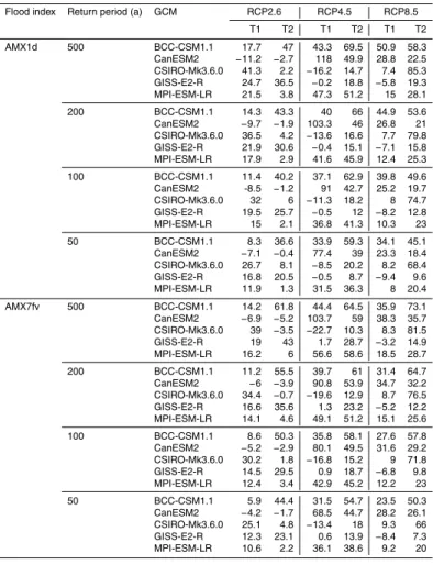
To further investigate the percentage changes in AMX1d and AMX7fv, four different

return periods (500a, 200a, 100a and 50a) were chosen (Table 2). Due to the uncer-tainty from GCMs, there is a relatively large variability in the results from the five GCMs. Nevertheless, most of GCMs project an increase during two future periods. As shown 10

in Table 2, the largest percentage change in AMX1d is found for the RCP4.5 scenario of the CanESM2 model in 2020–2050, with an increase of 118 % in the 500a return period, 103.3 % in the 200a return period, and 91.0 % in the 100a return period. In comparison, the largest percentage decline in AMX1d is mainly found for the RCP4.5 scenario of the CSIRO-Mk3.6.0 model in 2020–2050, with a decrease of 16.2 % in the 15

500a return period, 13.6 % in the 200a return period, and 11.3 % in the 100a return period. When considering the results from all future scenarios of the five models, the range of percentage changes are described here. For AMX1d, the percentage changes

in the 500-year return period range from -16.2 to 118 % in 2020–2050, and from−2.7

to 85.3 % in 2050–2080. For AMX7fv, the percentage changes in the 500-year return 20

period for AMX7fv range from−22.7 to 103.7 % in 2020–2050, and from−5.2 to 81.5 %

in 2050–2080 (Table 2).

4 Discussion

The impact of climate change on extreme floods in the Beijiang River basin were an-alyzed in this study, and the majority of modelling results informed by the five CMIP5 25

(14)

HESSD

11, 9643–9669, 2014

C. H. Wu et al.

Title Page

Tables Figures

◭ ◮

Back Close

Full Screen / Esc

Discussion

P

a

per

|

Discus

sion

P

a

per

|

Discussion

P

a

per

|

Discussion

P

a

per

|

Beijiang River basin would be “more likely than not” to increase under the RCP4.5 sce-nario. Based on four emission scenarios (A1B, RCP2.6, RCP4.5, and RCP8.5), Wu et al. (2014) found an increase of 4.35–9.18 % in the 500-year return period for daily discharge in the upstream of the Beijiang River basin. Evidence has been obtained to show that the Beijiang River basin is likely to experience an increase in episodes of 5

flooding in the following several decades.

In this study, we used five GCMs, three emission scenarios, ten downscaling simula-tions for each emission scenario, two stages of the future period and one hydrological model to discuss the possible range of projected changes in extreme floods. The re-sults indicate that GCMs and emission scenarios produce a large range of uncertainty 10

in flood projections in future climate conditions, which corroborates the previous find-ings of Chen et al. (2011), Kay et al. (2009), and Prudhomme and Davies (2009). In other words, the inconsistency in the projected changes (as produced by the various GCMs and the emission scenarios) highlights the impact of potential misleading con-clusions if only one GCM scenario were to be used for impact studies. Meanwhile, 15

it should be kept in mind that some other uncertainty sources, such as downscaling techniques and the hydrological model structure and its parameters, were overlooked in this study. Several previous studies have shown that the uncertainty sourced from the GCMs is much larger than those in downscaling techniques and hydrological mod-els (Prudhomme and Davies, 2009; Teng et al., 2012), although this does not imply that 20

uncertainty stemming from downscaling techniques and hydrological models should be ignored in impact studies. Taking the VIC model used in this study as an example, daily estimations of evapotranspiration (ET) in the model are made according to information received for relative humidity, wind speed, and long- and short-wave incoming radiation (Bohn et al., 2013). However, due to the limited coverage of meteorological data, VIC 25

is normally forced by daily data of maximum and minimum temperatures and precipi-tation, which is a common practice in many studies worldwide (e.g., Wu et al., 2014; Xiao et al., 2013). Pierce et al. (2013) found that this approach can result in opposite

(15)

HESSD

11, 9643–9669, 2014

C. H. Wu et al.

Title Page

Tables Figures

◭ ◮

Back Close

Full Screen / Esc

Discussion

P

a

per

|

Discus

sion

P

a

per

|

Discussion

P

a

per

|

Discussion

P

a

per

|

In addition, when using a hydrological model to assess the impact of climate change, there is an implicit assumption that the hydrological model parameters calibrated from observations remain valid for future climatic conditions (Xu et al., 2013). However, Merz et al. (2011) pointed that hydrological model parameters may potentially change if

cal-ibrated to different periods, and such a concept has important implications in climate

5

impact analyses. Therefore, a next step of this study is a thorough investigation of the uncertainty produced by hydrological model (VIC) structure and its parameters in the projection of impact of climate change on floods.

To highlight the uncertainty of the results, this paper attempts to describe the cred-ibility of projected flood changes with an approach using uncertainty expressions, as 10

recommended by the AR5. This provides a quantitative basis for estimating likelihoods for many aspects of future climate change. However, the results should be taken with care, as the likelihood scheme itself is inappropriate for use in subjective evaluation and needs to be supplemented with a qualitative framework (Risbey and Kandlikar, 2007). Use of a best combination of levels of confidence with likelihood, which pro-15

vides more powerful means for analysts to express uncertainty, should be considered in future work.

5 Conclusions

Based on five CMIP5 GCMs, this paper discusses the potential impacts of climate change on extreme floods in the Beijiang River basin. Two flood indexes (AMX1d and 20

AMX7fv) were chosen for use in analysis, and uncertainty in future flood trends was considered by using an uncertainty expressions approach.

Modeling results indicate that there are large uncertainties sourced from GCMs and emission scenarios. Overall, the uncertainty range for changes in historical extreme precipitation and flood magnitude can be well represented by the five GCMs. The 25

(16)

in-HESSD

11, 9643–9669, 2014

C. H. Wu et al.

Title Page

Tables Figures

◭ ◮

Back Close

Full Screen / Esc

Discussion

P

a

per

|

Discus

sion

P

a

per

|

Discussion

P

a

per

|

Discussion

P

a

per

|

creasing trends were found for the RCP4.5 scenario. There is a relatively large

variabil-ity in the projected ranges of AMX1d and AMX7fv under the different future scenarios

in the five GCMs, but most projected an increase during the two future periods (relative to the baseline period 1970–2000). Overall, the percentage changes in the 500-year

return period AMX1d ranged from −16.2 to 118 %, while the percentage changes in

5

the 500-year return period AMX7fv ranged from−22.7 to 103.7 %.

Acknowledgements. This study was supported by the National Basic Research Program of China (2010CB428405) and the Special Funds for Public Welfare Projects of the Ministry of Water Resources of China (201301093). The GCMs data were kindly provided by Zhiyong Wu and Heng Xiao from Hohai University.

10

References

Bennett, J. C., Grose, M. R., Corney, S. P., White, C. J., Holz, G. K., Katzfey, J. J., Post, D. A.,

and Bindoff, N. L.: Performance of an empirical bias-correction of a high-resolution climate

dataset, Int. J. Climatol., 34, 2189–2204, 2014.

Bohn, T. J., Livneh, B., Oyler, J. W., Running, S. W., Nijssen, B., and Lettenmaier, D. P.: Global 15

evaluation of MTCLIM and related algorithms for forcing of ecological and hydrological mod-els, Agric. For. Meteorol., 176, 38–49, 2013.

Chen, J., Brissette, F. P., Poulin, A., and Leconte, R.: Overall uncertainty study of the hydrolog-ical impacts of climate change for a Canadian watershed, Water Resour. Res., 47, W12509, doi:10.1029/2011WR010602, 2011.

20

Feyen, L., Dankers, R., Bódis, K., Salamon, P., and Barredo, J. I.: Fluvial flood risk in Europe in present and future climates, Clim. Change, 112, 47–62, 2012.

Fowler, H. J., Blenkinsop, S., and Tebaldi, C.: Linking climate change modelling to impacts stud-ies: recent advances in downscaling techniques for hydrological modelling, Int. J. Climatol., 27, 1547–1578, 2007.

25

(17)

HESSD

11, 9643–9669, 2014

C. H. Wu et al.

Title Page

Tables Figures

◭ ◮

Back Close

Full Screen / Esc

Discussion

P

a

per

|

Discus

sion

P

a

per

|

Discussion

P

a

per

|

Discussion

P

a

per

|

Hansen, M. C., Defries, R. S., Townshend, J. R. G., and Sohlberg, R.: Global land cover classi-fication at 1 km spatial resolution using a classiclassi-fication tree approach, Int. J. Remote Sens., 21, 1331–1364, 2000.

Huang, S., Hattermann, F. F., Krysanova, V., and Bronstert, A.: Projections of climate change

impacts on river flood conditions in Germany by combining three different RCMs with a

re-5

gional eco-hydrological model, Clim. Change, 116, 631–663, 2013.

IPCC: Climate Change 2013: The Physical Science Basis. Contribution of Working Group I to the Fifth Assessment Report of the Intergovernmental Panel on Climate Change, edited by: Stocker, T. F., Qin, D., Plattner, G.-K., Tignor, M., Allen, S. K., Boschung, J., Nauels, A., Xia, Y., Bex, V., and Midgley, P. M., Cambridge University Press, Cambridge, United Kingdom and 10

New York, NY, USA, 1535 pp., 2013.

Kay, A. L., Davies, H. N., Bell, V. A., and Jones, R. G.: Comparison of uncertainty sources for climate change impacts: flood frequency in England, Clim. Change, 92, 41–63, 2009. Kay, A. L. and Jones, D. A.: Transient changes in flood frequency and timing in Britain under

potential projections of climate change, Int. J. Climatol., 32, 489–502, 2012. 15

Kendall, M. G.: Rank Correlation Methods, 4th edn. Charles Griffin: London, UK, 1–202, 1975.

Li, H., Sheffield, J., and Wood, E. F.: Bias correction of monthly precipitation and temperature

fields from Intergovernmental Panel on Climate Change AR4 models using equidistant quan-tile matching, J. Geophys. Res.-Atmos., 115, D10101, doi:10.1029/2009JD012882, 2010. Liang, X., Lettenmaier, D. P., Wood, E. F., and Burges, S. J.: A simple hydrologically based 20

model of land surface water and energy fluxes for general circulation models, J. Geophys. Res.-Atmos., 99, 14415–14428, 1994.

Liu, L. L., Fischer, T., Jiang, T., and Luo, Y.: Comparison of uncertainties in projected flood frequency of the Zhujiang River, South China, Quatern. Int., 304, 51–61, 2013.

Mann, H. B.: Non-Parametric tests against trend, Econometrica, 13, 245–259, 1945. 25

Merz, R., Parajka, J., and Blöschl, G.: Time stability of catchment model param-eters: Implications for climate impact analyses, Water Resour. Res., 47, W02531, doi:10.1029/2010WR009505, 2011.

Mirza, M. M. Q., Warrick, R. A., and Ericksen, N. J.: The implications of climate change on floods of the Ganges, Brahmaputra and Meghna rivers in Bangladesh, Clim. Change, 57, 30

287–318, 2003.

(18)

HESSD

11, 9643–9669, 2014

C. H. Wu et al.

Title Page

Tables Figures

◭ ◮

Back Close

Full Screen / Esc

Discussion

P

a

per

|

Discus

sion

P

a

per

|

Discussion

P

a

per

|

Discussion

P

a

per

|

N., Riahi, K., Smith, S. J., Stouffer, R. J., Thomson, A. M., Weyant, J. P., and Wilbanks, T. J.:

The next generation of scenarios for climate change research and assessment, Nature, 463, 747–756, 2010.

Pennell, C. and Thomas, R.: On the Effective Number of Climate Models, J. Clim., 24, 2358–

2367, 2011. 5

Pierce, D. W., Westerling, A. L., and Oyler, J.: Future humidity trends over the western United States in the CMIP5 global climate models and variable infiltration capacity hydrological modeling system, Hydrol. Earth Syst. Sci., 17, 1833–1850, doi:10.5194/hess-17-1833-2013, 2013.

Pincus, R., Batstone, C. P., Hofmann, R. J. P., Taylor, K. E., and Glecker, P. J.: Evaluating the 10

present-day simulation of clouds, precipitation, and radiation in climate models, J. Geophys. Res.-Atmos., 113, D14209, doi:10.1029/2007JD009334, 2008.

Prudhomme, C. and Davies, H. N.: Assessing uncertainties in climate change impact analyses on river flow regimes in the UK. Part 2: future climate, Clim. Change, 93, 197–222, 2009.

Raff, D. A., Pruitt, T., and Brekke, L. D.: A framework for assessing flood frequency based on

15

climate projection information, Hydrol. Earth Syst. Sci., 13, 2119–2136, doi:10.5194/hess-13-2119-2009, 2009.

Risbey, J. S. and Kandlikar, M.: Expressions of likelihood and confidence in the IPCC uncer-tainty assessment process, Clim. Change, 85, 19–31, 2007.

Sachindra, D. A., Huang, F., Barton, A., and Perera, B. J. C.: Statistical downscaling of general 20

circulation model outputs to precipitation–part 1: calibration and validation, Int. J. Climatol., doi:10.1002/joc.3914, in press, 2014a.

Sachindra, D. A., Huang, F., Barton, A., and Perera, B. J. C.: Statistical downscaling of general circulation model outputs to precipitation–part 2: bias-correction and future projections, Int. J. Climatol., doi:10.1002/joc.3915, in press, 2014b.

25

Smith, I., Syktus, J., McAlpine, C., and Wong, K.: Squeezing information from regional climate change projections-results from a synthesis of CMIP5 results for south-east Queensland, Australia, Clim. Change, 121, 609–619, 2013.

Taylor, K. E., Stou_ffer, R. J., and Meehl, G. A.: An Overview of CMIP5 and the Experiment

Design, B. Am. Meteorol. Soc., 93, 485–498, 2012. 30

Teng, J., Vaze, J., Chiew, F. H. S., Wang, B., and Perraud, J.: Estimating the Relative Uncer-tainties Sourced from GCMs and Hydrological Models in Modeling Climate Change Impact

(19)

HESSD

11, 9643–9669, 2014

C. H. Wu et al.

Title Page

Tables Figures

◭ ◮

Back Close

Full Screen / Esc

Discussion

P

a

per

|

Discus

sion

P

a

per

|

Discussion

P

a

per

|

Discussion

P

a

per

|

Tisseuil, C., Vrac, M., Lek, S., and Wade, A. J.: Statistical downscaling of river flows, J. Hydrol., 385. 279–291, 2010.

Wang, G. Q., Zhang, J. Y., Jin, J. L., Pagano, T. C., Calow, R., Bao, Z. X., Liu, C. S., Liu, Y. L., and Yan, X. L.: Assessing water resources in China using PRECIS projections and a VIC model, Hydrol. Earth Syst. Sci., 16, 231–240, doi:10.5194/hess-16-231-2012, 2012.

5

Wu, C. H., Huang, G. R., Yu, H. J., Chen, Z. Q., and Ma, J. G.: Spatial and temporal distributions of trends in climate extremes of the Feilaixia catchment in the upstream area of the Beijiang River Basin, South China, Int. J. Climatol., doi:10.1002/joc.3900, in press, 2013a.

Wu, Z. Y., Lu, G. H., Liu, Z. Y., Wang, J. X., and Xiao, H.: Trends of Extreme Flood Events in the Pearl River Basin during 1951–2010, Adv. Climate Change Res., 4, 110–116, 2013b. 10

Wu, C., Huang, G., Yu, H., Chen, Z., and Ma, J.: Impact of climate change on reservoir flood control in the upstream area of the Beijiang River Basin, South China, J. Hydrometeor., doi:10.1175/JHM-D-13-0181.1, in press, 2014.

Xiao, H., Lu, G. H., Wu, Z. Y., and Liu Z. Y.: Flood response to climate change in the Pearl River basin for the next three decades, J. Hydraul. Eng., 12, 1409–1419, 2013 (in Chinese). 15

(20)

HESSD

11, 9643–9669, 2014

C. H. Wu et al.

Title Page

Tables Figures

◭ ◮

Back Close

Full Screen / Esc

Discussion

P

a

per

|

Discus

sion

P

a

per

|

Discussion

P

a

per

|

Discussion

P

a

per

|

Table 1.Percentage of samples with increasing trends of AMX1d and AMX7fv in future periods

based on five GCMs.

Flood index Emissions scenarios 2020–2050 2050–2080

IT SIT IT SIT

AMX1d

RCP2.6 60 10 74 10

RCP4.5 44 2 38 2

RCP8.5 54 2 72 8

AMX7fv

RCP2.6 60 8 68 10

RCP4.5 44 2 44 0

RCP8.5 58 2 62 10

(21)

HESSD

11, 9643–9669, 2014

C. H. Wu et al.

Title Page

Tables Figures

◭ ◮

Back Close

Full Screen / Esc

Discussion

P

a

per

|

Discus

sion

P

a

per

|

Discussion

P

a

per

|

Discussion

P

a

per

|

Table 2.Percentage changes (%) in AMX1d and AMX7fv under different scenarios (relative to

the baseline period 1970–2000).

Flood index Return period (a) GCM RCP2.6 RCP4.5 RCP8.5 T1 T2 T1 T2 T1 T2 AMX1d 500 BCC-CSM1.1 17.7 47 43.3 69.5 50.9 58.3 CanESM2 −11.2 −2.7 118 49.9 28.8 22.5

CSIRO-Mk3.6.0 41.3 2.2 −16.2 14.7 7.4 85.3

GISS-E2-R 24.7 36.5 −0.2 18.8 −5.8 19.3 MPI-ESM-LR 21.5 3.8 47.3 51.2 15 28.1 200 BCC-CSM1.1 14.3 43.3 40 66 44.9 53.6 CanESM2 −9.7 −1.9 103.3 46 26.8 21

CSIRO-Mk3.6.0 36.5 4.2 −13.6 16.6 7.7 79.8 GISS-E2-R 21.9 30.6 −0.4 15.1 −7.1 15.8 MPI-ESM-LR 17.9 2.9 41.6 45.9 12.4 25.3 100 BCC-CSM1.1 11.4 40.2 37.1 62.9 39.8 49.6 CanESM2 -8.5 −1.2 91 42.7 25.2 19.7

CSIRO-Mk3.6.0 32 6 −11.3 18.2 8 74.7 GISS-E2-R 19.5 25.7 −0.5 12 −8.2 12.8 MPI-ESM-LR 15 2.1 36.8 41.3 10.3 23 50 BCC-CSM1.1 8.3 36.6 33.9 59.3 34.1 45.1 CanESM2 −7.1 −0.4 77.4 39 23.3 18.4

CSIRO-Mk3.6.0 26.7 8.1 −8.5 20.2 8.2 68.4 GISS-E2-R 16.8 20.5 −0.5 8.7 −9.4 9.6 MPI-ESM-LR 11.9 1.3 31.5 36.3 8 20.4 AMX7fv 500 BCC-CSM1.1 14.2 61.8 44.4 64.5 35.9 73.1 CanESM2 −6.9 −5.2 103.7 59 38.3 35.7

CSIRO-Mk3.6.0 39 −3.5 −22.7 10.3 8.3 81.5

GISS-E2-R 19 43 1.7 28.7 −3.2 14.9 MPI-ESM-LR 16.2 6 56.6 58.6 18.5 28.7 200 BCC-CSM1.1 11.2 55.5 39.7 61 31.4 64.7 CanESM2 −6 −3.9 90.8 53.9 34.7 32.2

CSIRO-Mk3.6.0 34.4 −0.7 −19.6 12.9 8.7 76.5 GISS-E2-R 16.6 35.6 1.3 23.2 −5.2 12.2 MPI-ESM-LR 14.1 4.6 49.1 51.2 15.1 25.6 100 BCC-CSM1.1 8.6 50.3 35.8 58.1 27.6 57.8 CanESM2 −5.2 −2.9 80.1 49.5 31.6 29.2

CSIRO-Mk3.6.0 30.2 1.8 −16.8 15.2 9 71.8 GISS-E2-R 14.5 29.5 0.9 18.7 −6.8 9.8 MPI-ESM-LR 12.4 3.4 42.9 45.2 12.2 23 50 BCC-CSM1.1 5.9 44.4 31.5 54.7 23.5 50.3 CanESM2 −4.2 −1.7 68.5 44.7 28.2 26.1 CSIRO-Mk3.6.0 25.1 4.8 −13.4 18 9.3 66 GISS-E2-R 12.3 23.1 0.6 13.9 −8.4 7.3 MPI-ESM-LR 10.6 2.2 36.1 38.6 9.2 20

(22)

HESSD

11, 9643–9669, 2014

C. H. Wu et al.

Title Page

Tables Figures

◭ ◮

Back Close

Full Screen / Esc

Discussion

P

a

per

|

Discus

sion

P

a

per

|

Discussion

P

a

per

|

Discussion

P

a

per

|

115° E 110° E

105° E 27° N

26° N 25° N 24° N 23° N 22° N 21° N

DEM (m) High : 2800 Low : 0

130° E 120° E 110° E 100° E 90° E 80° E 50° N

40° N

30° N

20° N

(23)

HESSD

11, 9643–9669, 2014

C. H. Wu et al.

Title Page Abstract Introduction Conclusions References Tables Figures ◭ ◮ ◭ ◮ Back Close

Full Screen / Esc

Printer-friendly Version Interactive Discussion Discussion P a per | Discus sion P a per | Discussion P a per | Discussion P a per | 1 9 7 0 -8 -2 3 1 9 7 2 -4 -1 4 1 9 7 3 -1 2 -5 1 9 7 5 -7 -2 8 1 9 7 7 -3 -1 9 1 9 7 8 -1 1 -9 1 9 8 0 -7 -1 1 9 8 2 -2 -2 1 1 9 8 3 -1 0 -1 4 1 9 8 5 -6 -5 1 9 8 7 -1 -2 6 1 9 8 8 -9 -1 7 1 9 9 0 -5 -1 0 1 9 9 1 -1 2 -3 1 1 9 9 3 -8 -2 2 1 9 9 5 -4 -1 4 1 9 9 6 -1 2 -4 1 9 9 8 -7 -2 7 0 2000 4000 6000 8000 10000 12000 14000 16000 18000 20000 Validation (1991-1999) NSE=0.91 RE=3.67% Disc ha rge ( m 3/s) Year-month-day Observed Simulated (a) Calibration (1969-1990) NSE=0.88 RE=11.88%

0 10 20 30 40 50

0 10 20 30 40 50 Obse rve d ( mm ) Simulated (mm) (b) R2 =0.9053 1:1 line

0 30 60 90 120 150 180 210 240

0 30 60 90 120 150 180 210 240 Obse rve d ( mm ) Simulated (mm) (c) R2 =0.9295 1:1 line

Figure 2. Comparison of the simulated and observed runoff during the period 1969–1999.

(a)A comparison of simulated and observed discharges;(b) a comparison of simulated and

observed maximum 1-day runoffdepth and(c)a comparison of simulated and observed

(24)

HESSD

11, 9643–9669, 2014

C. H. Wu et al.

Title Page

Tables Figures

◭ ◮

Back Close

Full Screen / Esc

Discussion

P

a

per

|

Discus

sion

P

a

per

|

Discussion

P

a

per

|

Discussion

P

a

per

|

Figure 3. ECDFs for observed and simulated (a) AMX1p, (b) AMX7p, (c) AMX1d and (d)

(25)

HESSD

11, 9643–9669, 2014

C. H. Wu et al.

Full Screen / Esc

Printer-friendly Version Interactive Discussion Discussion P a per | Discus sion P a per | Discussion P a per | Discussion P a per | B C C -C S M 1 .1 -R C P2 .6 B C C -C S M 1 .1 -R C P4 .5 B C C -C S M 1 .1 -R C P8 .5 C an E S M 2 -R C P2 .6 C an E S M 2 -R C P4 .5 C an E S M 2 -R C P8 .5 C S IR O -M k 3 .6 .0 -R C P2 .6 C S IR O -M k 3 .6 .0 -R C P4 .5 C S IR O -M k 3 .6 .0 -R C P8 .5 G IS S -E 2 -R -R C P2 .6 G IS S -E 2 -R -R C P4 .5 G IS S -E 2 -R -R C P8 .5 M PI -E S M -L R -R C P2 .6 M PI -E S M -L R -R C P4 .5 M PI -E S M -L R -R C P8 .5 0 1 2 3 4 5 6 7 8 9 10 11 Number of samples GCM-scenario (a) B C C -C S M 1 .1 -R C P 2 .6 B C C -C S M 1 .1 -R C P 4 .5 B C C -C S M 1 .1 -R C P 8 .5 C an E S M 2 -R C P 2 .6 C an E S M 2 -R C P 4 .5 C an E S M 2 -R C P 8 .5 C S IR O -M k 3 .6 .0 -R C P 2 .6 C S IR O -M k 3 .6 .0 -R C P 4 .5 C S IR O -M k 3 .6 .0 -R C P 8 .5 G IS S -E 2 -R -R C P 2 .6 G IS S -E 2 -R -R C P 4 .5 G IS S -E 2 -R -R C P 8 .5 M P I-E S M -L R -R C P 2 .6 M P I-E S M -L R -R C P 4 .5 M P I-E S M -L R -R C P 8 .5 0 1 2 3 4 5 6 7 8 9 10 11 Num be r of sa m pl e s GCM-scenario

IT in 2020-2050 SIT in 2020-2050 IT in 2050-2080 SIT in 2050-2080 (b)

Figure 4.Number of the samples with increasing trends for(a)AMX1d and(b)AMX7fv under

different scenarios. IT indicates increasing trend. SIT indicates significant increasing trend at

(26)

HESSD

11, 9643–9669, 2014 Prediction of e xtreme floods based on CMIP5 c limate models C . H. W u et al. Title P age Abstr act Introduction Conclusions Ref erences T ab les Figures ◭ ◮ ◭ ◮ Bac k Close Full Screen / Esc Pr inter-fr iendly V ersion Inter activ e Discussion DiscussionP aper | Discussion Pa per | DiscussionP aper | DiscussionP aper | BCC-CSM1.1-Baseline BCC-CSM1.1-RCP2.6 BCC-CSM1.1-RCP4.5 BCC-CSM1.1-RCP8.5 CanESM2-Baseline CanESM2-RCP2.6 CanESM2-RCP4.5 CanESM2-RCP8.5 CSIRO-Mk3.6.0-Baseline CSIRO-Mk3.6.0-RCP2.6 CSIRO-Mk3.6.0-RCP4.5 CSIRO-Mk3.6.0-RCP8.5 GISS-E2-R-Baseline GISS-E2-R-RCP2.6 GISS-E2-R-RCP4.5 GISS-E2-R-RCP8.5 MPI-ESM-LR-Baseline MPI-ESM-LR-RCP2.6 MPI-ESM-LR-RCP4.5 MPI-ESM-LR-RCP8.5 -6 0 0 0 0

6000 12000 18000 24000 30000 36000 42000 48000

(

a)

2020-2050

Discharge (m3

/s) BCC-CSM1.1-Baseline BCC-CSM1.1-RCP2.6 BCC-CSM1.1-RCP4.5 BCC-CSM1.1-RCP8.5 CanESM2-Baseline CanESM2-RCP2.6 CanESM2-RCP4.5 CanESM2-RCP8.5 CSIRO-Mk3.6.0-Baseline CSIRO-Mk3.6.0-RCP2.6 CSIRO-Mk3.6.0-RCP4.5 CSIRO-Mk3.6.0-RCP8.5 GISS-E2-R-Baseline GISS-E2-R-RCP2.6 GISS-E2-R-RCP4.5 GISS-E2-R-RCP8.5 MPI-ESM-LR-Baseline MPI-ESM-LR-RCP2.6 MPI-ESM-LR-RCP4.5 MPI-ESM-LR-RCP8.5 -2

0 0 20 40 60 80 100 120 140 160 180 200 220

(

b)

2020-2050

100 million m3 BCC-CSM1.1-Baseline BCC-CSM1.1-RCP2.6 BCC-CSM1.1-RCP4.5 BCC-CSM1.1-RCP8.5 CanESM2-Baseline CanESM2-RCP2.6 CanESM2-RCP4.5 CanESM2-RCP8.5 CSIRO-Mk3.6.0-Baseline CSIRO-Mk3.6.0-RCP2.6 CSIRO-Mk3.6.0-RCP4.5 CSIRO-Mk3.6.0-RCP8.5 GISS-E2-R-Baseline GISS-E2-R-RCP2.6 GISS-E2-R-RCP4.5 GISS-E2-R-RCP8.5 MPI-ESM-LR-Baseline MPI-ESM-LR-RCP2.6 MPI-ESM-LR-RCP4.5 MPI-ESM-LR-RCP8.5 -6000 0

6000 12000 18000 24000 30000 36000 42000 48000 54000 60000 66000

2050-2080

Discharge (m3

/s) BCC-CSM1.1-Baseline BCC-CSM1.1-RCP2.6 BCC-CSM1.1-RCP4.5 BCC-CSM1.1-RCP8.5 CanESM2-Baseline CanESM2-RCP2.6 CanESM2-RCP4.5 CanESM2-RCP8.5 CSIRO-Mk3.6.0-Baseline CSIRO-Mk3.6.0-RCP2.6 CSIRO-Mk3.6.0-RCP4.5 CSIRO-Mk3.6.0-RCP8.5 GISS-E2-R-Baseline GISS-E2-R-RCP2.6 GISS-E2-R-RCP4.5 GISS-E2-R-RCP8.5 MPI-ESM-LR-Baseline MPI-ESM-LR-RCP2.6 MPI-ESM-LR-RCP4.5 MPI-ESM-LR-RCP8.5

-20 ₀ 20 40 60 80 100 120 140 160 180 200 220 240

2050-2080

100 million m3

(27)

HESSD

11, 9643–9669, 2014

C. H. Wu et al.

Full Screen / Esc

Printer-friendly Version Interactive Discussion Discussion P a per | Discus sion P a per | Discussion P a per | Discussion P a per |

0.01 1 10 40 70 95 99.5

0 5000 10000 15000 20000 25000 30000 35000 40000 45000 50000 (a) BCC-CSM1.1 Disc ha rge ( m 3/s) P (%) Baseline RCP2.6 2020-2050 RCP2.6 2050-2080 RCP4.5 2020-2050 RCP4.5 2050-2080 RCP8.5 2020-2050 RCP8.5 2050-2080

0.01 1 10 40 70 95 99.5

0 20 40 60 80 100 120 140 160 180 200 (b) BCC-CSM1.1 100 mi ll ion m 3 P (%) Baseline RCP2.6 2020-2050 RCP2.6 2050-2080 RCP4.5 2020-2050 RCP4.5 2050-2080 RCP8.5 2020-2050 RCP8.5 2050-2080

0.01 1 10 40 70 95 99.5

0 5000 10000 15000 20000 25000 30000 35000 40000 45000 50000 CanESM2 Disc ha rge ( m 3/s) P (%) Baseline RCP2.6 2020-2050 RCP2.6 2050-2080 RCP4.5 2020-2050 RCP4.5 2050-2080 RCP8.5 2020-2050 RCP8.5 2050-2080

0.01 1 10 40 70 95 99.5

0 20 40 60 80 100 120 140 160 180 200 CanESM2 100 mi ll ion m 3 P (%) Baseline RCP2.6 2020-2050 RCP2.6 2050-2080 RCP4.5 2020-2050 RCP4.5 2050-2080 RCP8.5 2020-2050 RCP8.5 2050-2080

0.01 1 10 40 70 95 99.5

0 10000 20000 30000 40000 50000 60000 70000 80000 CSIRO-Mk3.6.0 Disc ha rge ( m 3/s) P (%) Baseline RCP2.6 2020-2050 RCP2.6 2050-2080 RCP4.5 2020-2050 RCP4.5 2050-2080 RCP8.5 2020-2050 RCP8.5 2050-2080

0.01 1 10 40 70 95 99.5

0 50 100 150 200 250 300 350 400 CSIRO-Mk3.6.0 100 mi ll ion m 3 P (%) Baseline RCP2.6 2020-2050 RCP2.6 2050-2080 RCP4.5 2020-2050 RCP4.5 2050-2080 RCP8.5 2020-2050 RCP8.5 2050-2080

0.01 1 10 40 70 95 99.5

0 5000 10000 15000 20000 25000 30000 35000 40000 GISS-E2-R Disc ha rge ( m 3/s) P (%) Baseline RCP2.6 2020-2050 RCP2.6 2050-2080 RCP4.5 2020-2050 RCP4.5 2050-2080 RCP8.5 2020-2050 RCP8.5 2050-2080

0.01 1 10 40 70 95 99.5

0 20 40 60 80 100 120 140 160 GISS-E2-R 100 mi ll ion m 3 P (%) Baseline RCP2.6 2020-2050 RCP2.6 2050-2080 RCP4.5 2020-2050 RCP4.5 2050-2080 RCP8.5 2020-2050 RCP8.5 2050-2080

0.01 1 10 40 70 95 99.5

0 5000 10000 15000 20000 25000 30000 35000 40000 45000 50000 MPI-ESM-LR Disc ha rge ( m 3/s) P (%) Baseline RCP2.6 2020-2050 RCP2.6 2050-2080 RCP4.5 2020-2050 RCP4.5 2050-2080 RCP8.5 2020-2050 RCP8.5 2050-2080

0.01 1 10 40 70 95 99.5

0 20 40 60 80 100 120 140 160 180 200 MPI-ESM-LR 100 mi ll ion m 3 P (%) Baseline RCP2.6 2020-2050 RCP2.6 2050-2080 RCP4.5 2020-2050 RCP4.5 2050-2080 RCP8.5 2020-2050 RCP8.5 2050-2080

Figure 6.P-III frequency distributions of(a)AMX1d and(b)AMX7fv under different scenarios