NONLINEAR MODELS TO PREDICT NITROGEN MINERALIZATION IN AN OXISOL

NONLINEAR MODELS TO PREDICT NITROGEN

MINERALIZATION IN AN OXISOL

Janser Moura Pereira1_{; Joel Augusto Muniz}2_{*; Carlos Alberto Silva}3

1

UFLA - Pós-Graduando em Estatística e Experimentação Agropecuária. 2

UFLA - Depto. de Ciências Exatas, C.P. 37 - 37200-000 - Lavras, MG - Brasil. 3

UFLA - Depto. de Ciência do Solo.

*Corresponding author <joamuniz@ufla.br>

ABSTRACT: This work was carried out to evaluate the statistical properties of eight nonlinear models used to predict nitrogen mineralization in soils of the Southern Minas Gerais State, Brazil. The parameter estimations for nonlinear models with and without structure of autoregressive errors was made by the least squares method. First, a structure of second order autoregressive errors, AR(2) was considered for all nonlinear models and then the significance of the autocorrelation parameters was verified. Among the models, the Juma presented an autocorrelation of second order, and the model of Broadbent presented one of first order. In summary, these models presented significant autocorrelation parameters. To estimate the parameters of nonlinear models, the SAS procedure MODEL was used (SAS). The comparison of the models was made by measuring the fitted parameters: adjusted R-square, mean square error and mean predicted error. The Juma model with AR(2) best fitted for nitrogen mineralization without liming, followed by Cabrera, Stanford & Smith without autoregressive errors, for both with and without soil acidity correction.

Key words: autoregressive, estimators properties, mineralized nitrogen, variance, covariance matrices

MODELOS NÃO LINEARES PARA PREDIZER A MINERALIZAÇÃO

DE NITOGÊNIO NUM LATOSSOLO

RESUMO: Este trabalho teve por objetivo avaliar o grau do ajuste de oito modelos não lineares apresentados na literatura, utilizados para descrever a mineralização do nitrogênio em latossolo do sul de Minas Gerais incubado durante 28 semanas. A estimação dos parâmetros para os modelos de regressão não linear sem e com estrutura de erros autorregressivos foi feita pelo método de mínimos quadrados. A princípio, considerou-se para todos os modelos não lineares uma estrutura de erros autorregressivos de considerou-segunda ordem, AR(2) e, em seguida, verificou-se a significância dos parâmetros de autocorrelação. Apenas o modelo de Juma apresentou autocorrelação de segunda ordem, e o modelo de Broadbent apresentou autocorrelação de primeira ordem, ou seja, apenas estes modelos apresentaram parâmetros de autocorrelação significativos. Para estimação dos parâmetros dos modelos não lineares, utilizou-se o procedimento MODEL (SAS

). A comparação dos modelos foi feito por meio de critérios da qualidade do ajuste (coeficiente de determinação ajustado, quadrado médio do resíduo e erro de predição médio). O modelo de melhor ajuste foi o de Juma com AR(2), para a mineralização de N sem calagem, seguido pelos modelos de Cabrera, Stanford & Smith sem estrutura de erros autorregressivos, tanto para os dados com, quanto para aqueles obtidos sem a correção da acidez do solo.

Palavras-chave: autorregressivo, propriedades dos estimadores, nitrogênio mineralizado, matriz de variância, covariância

INTRODUCTION

Nitrogen is the most required nutrient by crops. The high cost and the large need of plants for nitrogen make N the most limiting nutrient for food production in the world. Nitrogen is found in soils predominantly in the organic form as a component of different soil or-ganic compounds. Compared to other nutrients, nitro-gen undergoes several transformations in soil which makes N availability to plants difficult to be evaluated. Mineralization is one of the N transformation processes in soils and it consists of the conversion of organic N into mineral N (ammonia), which under acid conditions

The evaluation of N availability may be achieved by means of short term biologic methods using soil sample incubation in laboratory as a basis for making N fertilizers recommendations for crops (Foth & Ellis, 1988). The incubation process consists of conditioning soils providing to the organisms associated to organic N conversion to ammonium the optimum conditions to ob-tain the maximum mineralization rates. Under controlled conditions, it is necessary to add water, nutrients, lime-stone and other inputs that limit the activity of izing organisms in order to evaluate the soil N mineral-ization potential as a function of time.

Mineralization of organic matter is higher during initial incubation periods due to the consumption by soil organisms of the most easily decomposable organic com-pounds (Gupta & Reuszer, 1967; Chew et al., 1976), and on account of the factors which may accelerate organic matter decomposition such as soil tillage processes, dry-ing, and grinding (Black, 1968).

Using empirical models it is possible to report and predict the relationships among events taking place in na-ture by fitting mathematical equations to experimental data (Camargo et al., 2002). To evaluate nitrogen mineraliza-tion dynamics in the soil, it is important to know which model best describes how this phenomenon is related to time. N mineralization in soil, according to Stanford & Smith (1972), may be described by a simple exponential model, which relates the mineralized N from a single po-tentially mineralizable N compartment to the incubation time, at a rate proportional to its concentration in soil. In other studies (Molina et al., 1980; Inobushi et al., 1985), the existence of two N compartments in the soil is taken into account, one with more and other with less mineral-ization potential, though Camargo et al., (2002) have re-jected the hypothesis of the existence of more than one N compartment in the soil, susceptible to mineralization.

In fertilization programs, most of the N required by crops is supplied by mineral fertilizers. When high amounts of N are added to soil, a great concern exists in relation to water and atmosphere pollution due to the in-efficient use of nitrogen fertilizers by plants which de-mands new alternatives that make possible the substitu-tion of all or part of those inputs (Scivittaro et al., 2000) and the better use of nitrogen supplied by soil through the mineralization process.

The prediction, by means of mathematical mod-els, of amounts of mineralized N over time, in soils un-der different management systems assumes great impor-tance relative to the following aspects: 1) allows the evaluation of soil capacity to supply N to plants; 2) makes the evaluation of mineral-N availability (nitrate + ammo-nia) possible in soils under different management sys-tems; 3) allows the determination of the best soil man-agement practices in order to increase the N use efficiency in the soil-plant system; 4) predicts the possibility of soil

contamination and quantificates nitrate fluxes to the wa-ter reservoirs; 5) furnishes the basis for defining correctly the N rates for different crops.

Based on Camargo et al. (2002), the present work proposes the matrix of variance and covariance param-eters of these models (Draper & Smith, 1998), consider-ing also autoregressive errors. To evaluate the degree of fitting of experimental data related to nitrogen mineral-ization in the Southern Minas Gerais State Oxisol incu-bated during 28 weeks in laboratory conditions, eight nonlinear models were chosen.

MATERIAL AND METHODS

Eight nonlinear models were evaluated by fitting experimental data associated with N mineralization in a Minas Gerais, (Brazil) Oxisol under the effect or not of liming. These data were obtained by Silva et al. (1994) and are related to the accumulated amounts of mineral-ized N during eleven incubation times (1, 2, 3, 4, 6, 8, 10, 12, 14, 21 and 28 weeks). Soil acidity correction was made in order to elevate the soil base saturation to 60% and the pH to values in the range of 6.0-6.2. Mineral N extraction (nitrate + ammonium) formed during incuba-tion was performed by periodic washing of the soil with a 0.01 mol L-1 CaCl₂ solution. The quantification of min-eralized N was performed in a steam draft distiller, with N-ammonium being quantified after addition of MgO in the CaCl₂ extract and nitrate after use of Devarda alloy in the remaining extract. Soil samples were incubated un-der laboratory conditions with air temperatures ranging between 21 and 28°C. The experimental design was com-pletely randomized with three replicates of 50 g of soil, with soil acidity corrected or not, mixed to 50 g of me-dium sand and incubated in funnels during 0 to 28 weeks. The mineralized amounts of N were accumulated in time (weeks). The nonlinear empirical models to predict N mineralization in relation to time (weeks) are presented in Table 1.

The description of the terms (parameters) in these models is as follows:

N_m is the mineralized nitrogen at time t; t is the incubation time (weeks); N₀ is the potentially mineraliz-able Nitrogen; h, k, k₀, k₁, k₂, k_q e k_s are mineralization rates; S is the least stable fraction of organic nitrogen; (1 - S) is the resistant fraction of organic nitrogen; N₁,

N_0q are the easily mineralizable N; N₂, N_0sare the hardly mineralizable N; A and b are constants; ε_~ a vector of er-rors with normal distributions with mean zero and vari-ance σ2_{. This structure of the errors was considered for}

the models with no autocorrelation in the residuals. For models which have residual autocorrelations a stationary autoregressive process of first order AR(1) was considered:

1 , 1 1,

t t t

in which

φ

t

ε

,the white noise (Hoffmann & Vieira, 1998).

If necessary a second order autoregressive pro-cess, AR(2), was considered (Morettin & Toloi, 2004):

1 2

1 2

t t t t

u =

φ

φ

ε

here

φ

2

φ

are autocorrelation parameters and

t

ε

is the white noise. The process is stationary if

1 2 1, 2 1 1 and 1 2 1.

φ φ

φ φ

φ

In studies using regression models, it is assumed that errors are independent. Generally the problem of autocorrelated errors appears with longitudinal data, in which the error of observation relative to one period is correlated with the error in the previous observation (Hoffman & Vieira, 1998). However, in the case of us-ing nonlinear models for the description of the index of soil nitrogen mineralization, it is important to consider autocorrelation since measures of accumulated nitrogen are taken at several times in the same plot, which make them likely to be correlated.

Simple exponential models consider the existence of only one “pool”, where the potentially mineralizable N, (N₀), is decomposed in a rate proportional to its concen-tration, while the double exponential models consider the existence of two “pools” or compartments. Thus, there are

two rates taking place in the process, one relative to the soil organic matter compartment that is more stable (resis-tant) and the other to the compartment that is less stable.

The hyperbolic model of Juma et al. (1984) pro-vides an estimate of the half life

( )

min-eralization (Camargo et al., 2002), while the parabolic model of Broadbent (1986) used by Stanford & Smith (1972) gives a pre-estimate of the potentially mineraliz-able nitrogen (N₀).

Estimates of the parameters for the nonlinear models with and without AR(1) and AR(2) error struc-tures were obtained only for the models that have shown autocorrelation in residuals. The least squares estimation of the parameters was made using the iterative algorithm of Marquardt (1963), implemented in the PROC MODEL (SAS®, 1999) statistic software. The nonlinear models were evaluated using the mean square error MSE (Draper & Smith, 1998), the adjusted coefficient of determination,

Adj R2, (Draper & Smith, 1998) and the mean prediction error, MPE, (Mazzini et al., 2005).

RESULTS AND DISCUSSION

After models were fitted to the experimental re-sults, with and without liming, first considering the mod-els without autoregressive errors, modmod-els AR(1) and

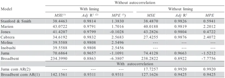
Table 2 - Nonlinear model fitting with and without structure of autoregressive errors, with and without liming.

1 _{MSE Mean Square Error;} 2 _{Adj R}2_{: Adjusted coefficient of determination;} 3_{MPE: Mean Predicted Error.}

l e d o M n o i t a l e r r o c o t u a t u o h t i W g n i m i l h t i

W Withoutliming

S

M E(1) _AdjR2(2) _MPE (3_{) MSE AdjR}2 _MPE

h t i m S & d r o f n a t

S 38.4463 0.9814 1.3830 38.4870 0.9826 0.5941 n

o i r a

M 43.0722 0.9791 1.7016 40.0188 0.9819 2.2012 s

e n o

J 41.4207 0.9799 -0.1028 43.2826 0.9804 0.4722 a r e r b a

C 34.6192 0.9832 2.5683 27.4255 0.9876 2.4072 a

n i l o

M 39.5588 0.9808 2.5496 --- --- --

-i h s u b o n

I 39.5588 0.9808 2.5456 --- --- --

-a m u

J 70.6864 0.9657 -1.1091 74.4128 0.9663 -1.5212 t n e b d a o r

B 234.3990 0.8863 -6.3807 238.2822 0.8922 -7.7756 n o i t a l e r r o c o t u a h t i W ) 2 ( R A m o c a m u

J --- --- --- 17.7257 0.9920 0.9920

) 1 ( R A m o c t n e b d a o r

B 142.1561 0.9311 0.9311 127.1626 0.9425 0.9425 l

e d o

M Equation Reference

l a i t n e n o p x e e l p m i S )

a N_m=N₀[1-exp(-kt)] +ε Stanford&Smith(1972) l a i t n e n o p x E e l p m i S )

b N_m=N₀[1-exp(-ktb_{)]+ε Marionetal.(1981)}

l a i t n e n o p x E e l p m i S )

c N_m=N₁+N₂-[N₂exp(-k₂t)]+ε _Jones(1984)

l a i t n e n o p x E e l p m i S )

d N_m=N₁[1-exp(-k₁t)]+k₀t+ε Cabrera(1993) l a i t n e n o p x E e l b u o D )

e N_m=N₀S[1-exp(-ht)]+N₀(1-S)[1-exp(-kt)] +ε Molinaetal. (1980) l a i t n e n o p x E e l b u o D )

f N_m=N_0q[1-exp(-k_qt)]+N_0s[1-exp(-k_st)]+ε Inobushietal. (1985) c i l o b r e p y H )

g N_m=(N₀t)/( +t)+ε _{Jumaetal. (1984)}

c i l o b a r a P )

h N_m=Atb_{+ε Broadbent(1986)}

Table 1 - Nonlinear models for the mineralization of soil N related to time (weeks).

t

t

ε

2

AR(2) for residuals were fitted, when necessary. The pro-cess verified whether a model contains autocorrelated er-rors, i.e., it analyzed the significance of the respective autocorrelation parameter.

Table 2 summarizes the analyses with and with-out autoregressive errors. Cabrera’s and Stanford & Smith’s models presented the lowest values for the MSE

for data with and without liming. In Juma’s AR(2) and Broadbent’s AR(1) models, with and without liming, there was a decrease in the MSE.

Values of Adj R2 for the models without autoregressive residuals, except for Juma and Broadbent, were superior to 0.97. This denotes a good fit. The al-lowance of the autocorrelation in residuals provided an

increase in Adj R2

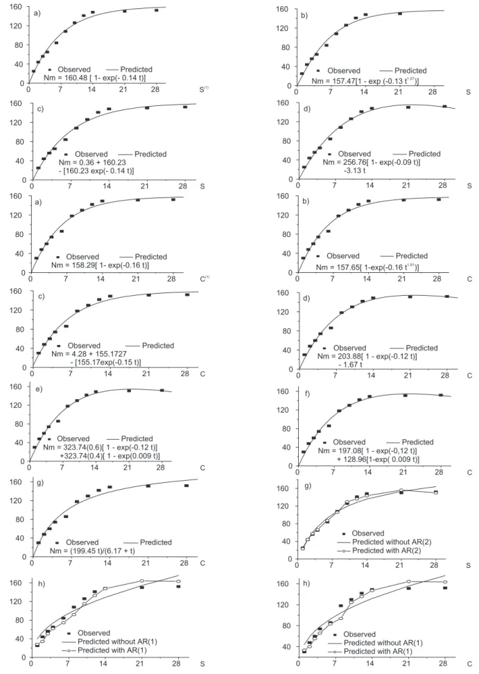
for Juma’s model with AR(2), without liming. It fitted well presenting an Adj R2 higher than 0.99. Broadbent’s model with AR(1) errors provided an increase in, but lower than 0.95, this is shown in Figure 1 (the two last plots (h)).

Accordingly to the mean predicted error (MPE) for the models without autoregressive errors (Table 2), Jones’ model, followed by Stanford & Smith’s for the cul-tivation situation without liming, presented the best fits, while Juma and Broadbent’s overestimated (negative sig-nal) the observed values. For cultivation with liming, Jones’ model presented the best fit. Cabrera, Molina, Inobushi, Marion and Stanford & Smith underestimated (positive signal) the observed values and the models of

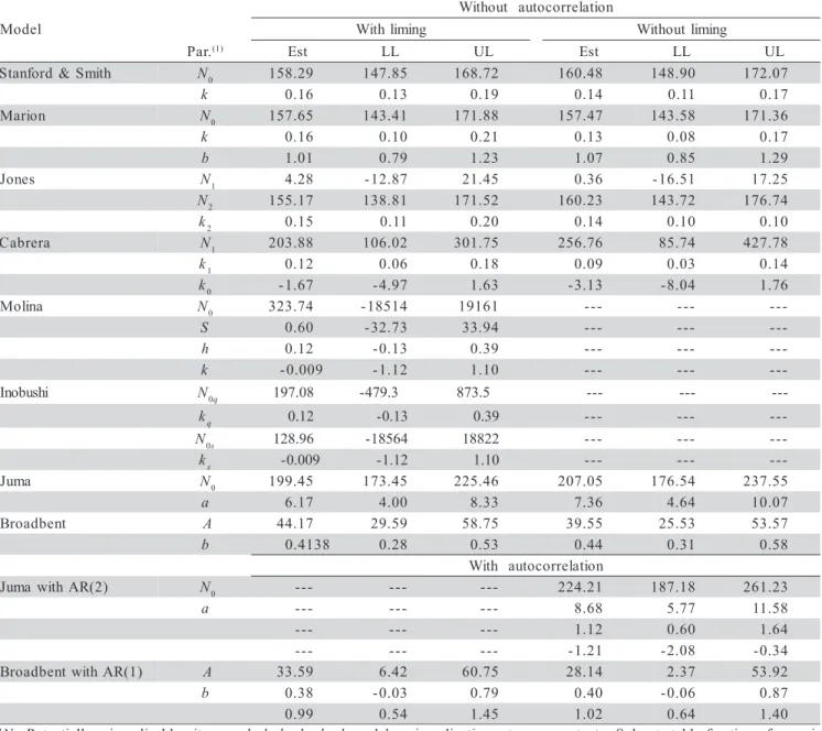
Table 3 - Parameters estimates (Est) lower confidence interval limits (LL), upper limits (UL) for models with and without structure of autoregressive errors, with and without liming.

1_N

0: Potentially mineralizable nitrogen; h, k, k0, k1, k2, kq and ks: mineralization rates or constants; S: least stable fraction of organic

nitrogen; N₁, N_0q: easily mineralizable nitrogen N; N₂, N_0s: N hardly mineralizable N; A and b: constants; φ1 and : autocorrelation

parameters. l e d o M

n o i t a l e r r o c o t u a t u o h t i W g n i m i l h t i

W Withoutliming

. r a

P (1) _{Est LL UL Est LL UL}

h t i m S & d r o f n a t

S N₀ 158.29 147.85 168.72 160.48 148.90 172.07

k 0.16 0.13 0.19 0.14 0.11 0.17

n o i r a

M N₀ 157.65 143.41 171.88 157.47 143.58 171.36

k 0.16 0.10 0.21 0.13 0.08 0.17

b 1.01 0.79 1.23 1.07 0.85 1.29

s e n o

J N₁ 4.28 -12.87 21.45 0.36 -16.51 17.25

N₂ 155.17 138.81 171.52 160.23 143.72 176.74

k₂ 0.15 0.11 0.20 0.14 0.10 0.10

a r e r b a

C N₁ 203.88 106.02 301.75 256.76 85.74 427.78

k₁ 0.12 0.06 0.18 0.09 0.03 0.14

k₀ -1.67 -4.97 1.63 -3.13 -8.04 1.76

a n i l o

M N₀ 323.74 -18514 19161 --- --- --

-S 0.60 -32.73 33.94 --- --- --

-h 0.12 -0.13 0.39 --- --- --

-k -0.009 -1.12 1.10 --- --- --

-i h s u b o n

I N_0q 197.08 -479.3 873.5 --- --- --

-k_q 0.12 -0.13 0.39 --- --- --

-N_0s 128.96 -18564 18822 --- --- --

-k_s -0.009 -1.12 1.10 --- --- --

-a m u

J N₀ 199.45 173.45 225.46 207.05 176.54 237.55

a 6.17 4.00 8.33 7.36 4.64 10.07

t n e b d a o r

B A 44.17 29.59 58.75 39.55 25.53 53.57

b 0.4138 0.28 0.53 0.44 0.31 0.58

n o i t a l e r r o c o t u a h t i W )

2 ( R A h t i w a m u

J N₀ --- --- --- 224.21 187.18 261.23

a --- --- --- 8.68 5.77 11.58

-- --- --- 1.12 0.60 1.64

-- --- --- -1.21 -2.08 -0.34 )

1 ( R A h t i w t n e b d a o r

B A 33.59 6.42 60.75 28.14 2.37 53.92

b 0.38 -0.03 0.79 0.40 -0.06 0.87

9 9 .

Figure 1 - Comparison of models to estimate potentially mineralizable N. Letters in lower case correspondent to the models reported in Table 1. 1_{C = with liming; S = without liming.}

Time (weeks)

S(1)

0 7 14 21 28

0 40 80 120 160

a)

Observed Predicted

Nm = 160.48 [ 1- exp(- 0.14 t)]

0 7 14 21 28

0 40 80 120 160

Observed Predicted

Nm = 157.47[1 - exp (-0.13 t1.07)] b)

S

0 7 14 21 28

0 40 80 120 160

Observed Predicted

Nm = 0.36 + 160.23 - [160.23 exp(- 0.14 t)] c)

S 00 7 14 21 28

40 80 120 160

Observed Predicted

Nm = 256.76[ 1- exp(-0.09 t)] -3.13 t

d)

S

0 7 14 21 28

0 40 80 120 160

Observed Predicted

Nm = 158.29[ 1- exp(-0.16 t)] a)

C(1)

0 7 14 21 28

0 40 80 120 160

Observed Predicted

Nm = 157.65[ 1-exp(-0.16 t1.01)] b)

C

C

0 7 14 21 28

0 40 80 120 160

Observed Predicted

Nm = 4.28 + 155.1727 - [155.17exp(-0.15 t)] c)

0 7 14 21 28

0 40 80 120 160

Observed Predicted

Nm = 203.88[ 1 - exp(-0.12 t)] - 1.67 t

d)

C

0 7 14 21 28

0 40 80 120 160

Observed Predicted

Nm = 323.74(0.6)[ 1 - exp(-0.12 t)] +323.74(0.4)[ 1 - exp(0.009 t)] e)

C

0 7 14 21 28

0 40 80 120 160

Observed Predicted

Nm = 197.08[ 1 - exp(-0,12 t)] + 128.96[1-exp( 0.009 t)] f)

C

C

0 7 14 21 28

0 40 80 120 160

Observed Predicted

Nm = (199.45 t)/(6.17 + t) g)

0 7 14 21 28

0 40 80 120 160

Observed

Predicted without AR(2) Predicted with AR(2) g)

S

0 7 14 21 28

0 40 80 120 160

Observed

Predicted without AR(1) Predicted with AR(1) h)

S 0 7 14 21 28

40 80 120 160

Observed

Predicted without AR(1) Predicted with AR(1) h)

C

Mineralized N, mg of N kg

Juma and Broadbent overestimated them. The models with autoregressive errors, Juma with AR(2) and Broadbent with AR(1), underestimated the observed val-ues, i.e., presented positive signal (Table 2).

Jones’ model, in both situations (with and with-out liming) has confidence intervals for the parameter in-cluding zero, which means that this parameter is not sig-nificant for the data under study (Table 3). Therefore, Jones’ model has a structural form equivalent to the Stanford & Smith’s model. Models of Molina and Inobushi also have confidence intervals of parameters containing zero (Table 3). From the standpoint of infer-ence, the parameters could be zero, with no fit. Another aspect of lack of fit is that the intervals of the parameters presented large ranges.

CONCLUSIONS

Autocorrelated errors were verified only in Juma’s model without liming and in Broadbent’s model, for soil samples with and without liming. The introduc-tion of autocorrelaintroduc-tion improved the fit only for Juma’s model with AR(2) without liming.

The mathematical model that best described the N mineralization dynamics is that one proposed by Juma with AR(2) in soils sample without soil acidity correc-tion followed by Cabrera’s, Stanford & Smith’s models without an autoregressive error structure, for both types of soil.

The model which provided the worst fit was Broadbent’s with and without autoregressive error struc-ture, with and without liming.

ACKNOWLEDGEMENTS

To CNPq for the financial support and scholar-ships.

REFERENCES

BLACK, C.A. Soil-plant relationships. New York: John Wiley, 1968. 792p. BROADBENT, F.E. Empirical modeling of soil nitrogen mineralization.

Soil Science, v.141, p.208-213, 1986.

CABRERA, M.L. Modeling the flush of nitrogen mineralization caused by drying and rewetting soils. Soil Science Society of America Journal, v.57, p.63-66, 1993.

CAMARGO, F.A. de O.; GIANELLO, C.; TEDESCO, M.J.; RIBOLDI, J.; MEURER, E.J.; BISSANI, C.A. Empirical models to predict soil nitrogen mineralization. Ciência Rural, v.32, p.393-399, 2002.

CHEW, W.Y.; WILLIAMS, C.N.; JOSEPH, K.T.; RAMLI, K. Studies on the availability to plants of soil nitrogen in Malaysian tropical oligotrophic peat. I – Effect of liming and pH. Tropical Agriculture,

v.53, p.69-78, 1976.

DRAPER, N.R.; SMITH, H. Applied regression analysis. 3.ed. New York: John Wiley & Sons, 1998. 706p.

FOTH, H.D.; ELLIS, B.G. Soil fertility. New York; John Wiley & Sons, 1988. 212p.

GUPTA, U.C.; REUSZER, H.W. Effect of plant species on the aminoacid content and nitrification of soil organic matter. Soil Science, v.104, p.395-400, 1967.

HAYNES, R.J. Mineral nitrogen in the plant-soil system. Orlando; Academic Press, 1986. 483 p.

HOFFMANN, R.; VIEIRA, S. Análise de regressão: uma introdução à econometria. 3.ed. São Paulo: HUCITEC, 1998. 379p.

INOBUSHI, K.; WADA, H.; TAKAI, Y. Easily decomposable organic matter in paddy soil. VI. Kinetics of nitrogen mineralization in submerged soils.

Journal of Soil Science and Plant Nutrition, v.34, p.563-572, 1985. JONES, A. Estimation of an active fraction soil nitrogen. Communications

in Soil Science and Plant Analysis, v.15, p.23-32, 1984.

JUMA, N.G.; PAUL, E.A.; MARY, B. Kinetic analysis of net mineralization in soil. Soil Science Society of America Journal, v.48, p.465-472, 1984. MARION, G.M.; KUMMEROW, J.; MILLER, P.C. Predicting nitrogen mineralization in chaparral soils. Soil Science Society of America Journal, v.45, p.956-961, 1981.

MARQUARDT, D.W. An algorithm for minimumsquares estimation of non-linear parameters. Journal of Society of Applied Mathematic, v.11, p.431-441, 1963.

MAZZINI, A.R. de A.; MUNIZ; J.A.; SILVA, F.F.; AQUINO, L.H. Curva de crescimento de novilhos Hereford: heterocedasticidade e resíduos autorregressivos. Revista Ciência. Rural, v.35, p.422-427, 2005. MOLINA, J.A.E.; CLAPP, C.E.; LARSON, W.E. Potentially mineralizable

nitrogen in soil: the simple exponential model does not apply for the first 12 weeks of incubation. Soil Science Society of American Journal,

v.44, p.442-443, 1980.

MORETTIN, P.A.; TOLOI, C.M. de C. Análise de séries temporais. São Paulo: Edgard Blucher, 2004. 534p.

NYBORG, M.; HOYT, P.B.; PENNY, D.C. Ammonification and nitrification of N in soils at 26 field sites one year after liming. Communications in Soil Science and Plant Analysis, v.19, p.1371-1379, 1988.

SAS INSTITUTE INC. SAS/STAT User‘s Guide. Version 18 Cary: SAS Institute, 1999.

SCIVITTARO, W.B.; MURAOKA, T.; BIARETTO, A.E.; TRIVELIN, P.C.O. Utilização de nitrogênio de adubos verde e mineral pelo milho.

Revista Brasileira de Ciência do Solo, v.24, p.917-926, 2000. SILVA, C.A.; VALE, F.R.; GUILHERME, L.R. Efeito da calagem na

mineralização do nitrogênio em solos de Minas Gerais. Revista Brasileira Ciência do Solo, v.18, p.471-476, 1994.

STANFORD, G.; SMITH, S.J. Nitrogen mineralization potentials of soils.

Soil Science of America Journal Proceedings, v.36, p.465-472, 1972.