*UEPA, Belém, PA, Brasil Received 07/03/2012, Accepted 10/02/2013
Network modelling of palm biodiesel plants to supply
the isolated electric power systems of Pará state
Thassyo Jorge Gonçalves Pereiraa*, Cláudio Mauro Vieira Serrab,
André Cristiano Silva Meloc, Najmat Celene Nasser Medeiros Brancod
a*[email protected], UEPA, Brasil b[email protected], UEPA, Brasil c [email protected], UEPA, Brasil d[email protected], PUC-Rio, Brasil
Abstract
Despite the great advance brought by the National Interconnected System (NIS), which is able to provide clean hydroelectric power to almost all Brazilian customers, there are still cities supplied by power generated from fossil fuel, which are subsidized by taxes, they are called Isolated Electric Power Systems (IEPS). Pará State, that has 34 cities with IEPS, also has potential to crop raw material (palm and sugar cane) to produce biodiesel for power generation. Our study analyzes the supply and distribution network of biodiesel under some scenarios of waterways availability, considering that they are also source of power to the NIS by the construction of hydroelectric dams. We develop specific demand and facility location models and apply them to the scenarios. Our results point to the efficiency of the generated models, the importance of three cities for the network, and to the little impact of some waterways in the total transportation costs.
Keywords
Capacitated facility location problem. Pará state isolated electric power systems. Palm biodiesel.
1. Introduction
The Brazilian National Electric Power System is divided into two geo-electric regions: the big one, with 60% of the national territory and 97.6% of the power market, referred as the National Interconnected System (NIS), and the little one, with 340 isolated power systems, 40% of the territory, and 2.4% of the power market, called Isolated Electric Power Systems (IEPS) (CONDE, 2006).
Most of NIS’s electric power comes from hydroelectric plants and is transmitted by high-voltage networks. These networks allow the power to be traded among the NIS’s subsystems: Southern Region, Southeastern Region, most of Northeastern and Central Western Region, and part of Pará State. IEPS’s power is mostly of thermal origin (diesel and fuel oil), transmitted by short power grids to no more than one city. There are IEPS in the States of Acre, Amazonas, Amapá, Rondônia, Roraima, part
of Pará and Mato Grosso and three locations in the Northeastern Region (SANTOS, 2008).
IEPS generally have low supply quality and high operation costs, mainly because of (CONDE et al., 2009):
a) Customers are very far from each other (average of 1 customer/km²);
b) Difficult supply logistics, with few roads in good conditions;
c) Poor communication system, which makes it hard to manage the system;
The recent growth in the IEPS’s fossil fuel consume has been discussed among the Government and power sector planners due to concerns about the Fuels Consume Tax (FCT). This federal subside aims to equalize the high generation costs of thermal power to the costs of NIS’s power (SANTOS, 2008). The FCT is considered the major tax in the NIS’s power bill (SANTOS, 2008). All the NIS electric power dealers must contribute to the FCT with a monthly share, proportional to its market size, in such a way that all the Brazilian customers pay for most of the IEPS’s fuel (CONDE, 2006).
The concerns over FCT and the IEPS’s low supply quality when associated with the global warning discussions motivate the search for alternative energy sources, able to reduce the regional dependency of fossil fuels and lower the national taxes. The fuels obtained from the extraction and processing of biomass, such as forest and agro-industry residues, vegetable oils, and biodiesel rank among the top alternatives to the IEPS of the Northern Region (SANTOS, 2008).
Biodiesel is an ester of fatty acids, substitute of mineral diesel. It has cleaner combustion and is obtained from renewable natural sources such as vegetable fats and oils. As the mineral diesel, it is used in internal combustion engines and can be blended with the latter (Bn, with n standing for the biodiesel percentage in the mixture) or pure (B100), requiring few modifications in the engine (UDAETA et al., 2004). B100’s efficiency is about 94% of the mineral diesel (SILVA et al., 2006).
Biodiesel is obtained mainly from transesterification, which is the reaction of vegetable oils with an active intermediate, created by the reaction of a short chain alcohol (ethanol or methanol) with a catalyst (UDAETA et al., 2004). The balance of the chemical equation with ethanol receives 954kg of vegetable oil (87% of the entrance) to react with 140kg of alcohol (13% of the entrance), yielding 1000kg of biodiesel and 94kg of glycerin (DAVARIZ, 2006).
Palm oil and sugar cane were the second and third agricultural commodities more produced in Pará State in 2007, with a production of about 870,000 and 667,000 tons, respectively. Tailândia (palm oil) and Ulianópolis (sugar cane) ranked as the main producers (FUNDAÇÃO..., 2009). There is at least one company producing ethanol in the latter (OLIVEIRA et al., 2007).
The raw material availability plus the existence of 34 IEPS fueled by diesel oil in Pará State creates the possibility for these systems to be supplied by local biodiesel. Our studies aims at modeling Pará’s IEPS’s biodiesel demand for 2011 and apply a facility
location model to determine optimal places and sizes of biodiesel plants to supply all the IEPS.
For the demand forecast, we will use a top-down approach of Holt-Winters multiplicative model to forecast the diesel demand, and use that to obtain the biodiesel demand forecast.
For the biodiesel plants location, we will develop, based on the Capacitated Facility Location Problem (CFLP), one model that considers the transportation costs from the plants to the customers, the transportation costs of the raw materials (palm oil and ethanol) to the plants, the size and fixed costs of the biodiesel plants.
The remainder of the paper is organized as follows. In Section 2 there is a literature review abut the demand forecast and facility location concepts used in our study. In Sections 3 and 4 we develop the demand forecast and the facility location models that we use, respectively. In Section 5 we present and treat the data to be inputted into the models. In Section 6 we present the results obtained in all the waterways availability scenarios, and discuss the impact of the hydroelectric plants’ dams over the transportation costs. In Section 7, we finish the paper with our conclusions and suggestions for future studies.
2. Literature review
Demand forecast and facility location are strategic decisions for the supply chain, having strong impact upon operational and tactical management levels. More specifically, facility location is the most important strategic decision, given its higher costs and its power to determine transportation conditions and inventory levels all over the network future operation (MONTEBELLER JÚNIOR; WANKE, 2009). Demand forecasting is the start point for the whole planning process, given that it defines which, how many and when the products will be consumed (DIAS, 2009).
2.1.
Time series forecast
The demand forecast models that consider the past demand, known as time series models, are suitable when the future demand is expected to follow historical patterns (CHOPRA; MEINDL, 2009). These models consider that the demand (Y) can be split into a systematic (Ŷ) and a random component (e), as (1).
Y – Ŷ + c (1)
smoothing constants, choosing the one that yields the smallest value of (6) (SEGURA; VERCHER, 2001). Whichever optimization method one wishes to use, the following problem must be solved:
( , , )
Minimizeϕ α β γ (6)
Subject to:
, , [0,1]
α β γ ∈ (7)
2.1.2.
Holt-Winters’ multiplicative
For this model, Koehler, Snyder and Ord (2001) define the Equations 8, 9, 10, and 11, that follow the same principles of the equations on Section 2.1.1.
^
( )
t n t t t n p
Y+ = E +nT S+ − (8)
(
1)
( 1 1)t
t t t
t p
Y
E E T
S
α α − −
−
= + − +
(9)
(
1)
(
1)
1t t t t
T =β E −E− + −βT− (10)
(
1)
t
t t p
t
Y
S S
E
γ γ −
= + −
(11)
2.1.3.
Forecast errors
The error measure of one forecast is important to: estimate its random component, identify whether the forecast model is inadequate (CHOPRA; MEINDL, 2009), and to determine the values of the smoothing constants. Segura and Vercher (2001) mention the root mean square error (RMSE), given by (12), as an often used error measure. This equation is what one wishes to minimize at (6).
2 1( )
n
t t
t Y Y
RMSE
n
= −
=
∑
(12)
The identification of whether the forecast model is inadequate, means to check if it is able to properly forecast the systematic component (e.g. if pessimist or optimistic errors are not being generated), and generate IID errors. The errors are the difference among the forecasted values and the actual values of all the t periods, which is given by (13). The Durbin-Watson statistic (d) analyzes the relationship among the errors considered random and independent variables – called
the random component (BROCKWELL; DAVIS, 2002). An often used method to obtain the systematic component is the exponential smoothing, which is very effective in reducing the amount of data to be handled and the computer effort. It is based on the periodic update of up to three systematic components through smoothing constants (SEGURA; VERCHER, 2001).
i) Level (E, constant mean horizontal demand), called simple exponential smoothing;
ii) Level and trend (T, when the mean demand increases or decreases with time), called double exponential smoothing or Holt’s method (HOLT, 1957, 2004); iii) Level, trend, and seasonality (S, when the demand
oscillates periodically), called triple exponential smoothing or Holt-Winters’ method (WINTERS, 1960).
The elements of Holt-Winters’ method can be arranged in two ways: additive or multiplicative. Each of them respectively represent the seasonality’s independency or dependency of the local mean (LAWTON, 1998).
2.1.1.
Holt-Winters’ additive
Considering the demand periodicity as p, and as n the number of periods ahead of the period t that one wishes to forecast, Lawton (1998) states that (2) yields the forecast value for the period t + n.
^
t n Et nTt t n p
Y+ = + +S+ − (2)
Level, trend and seasonality are given by (3), (4), and (5).
(
)
(
1)
( 1 1)t t t p t t
E =α Y−S− + −α E− +T− (3)
(
1)
(
1)
1t t t t
T =β E −E− + −βT− (4)
(
)
(
1)
t t t t p
S =γ Y−E + −γ S− (5)
data behavior, but also the forecast goal. Top-down is useful to look at the big-picture (strategic decisions), and bottom-up behaves well to operational decisions (FERREIRA, 2006).
2.2.
Facility location problems
Facility location models address questions like the quantity and location of facilities and the demand distribution among them. In this sense, two important strategic measures for facilities location are their proximity to the customers and their capacities (JAYARAMAN, 1998). In fact, the average transportation distance was one of the first measures of the quality of the facility location (OWEN; DASKIN, 1998): by weighting the distance of some facility and its customers and the customers’ demand, Hakimi (1964) defined his P-Median model, considering:
• j: index of some potential facility site, • k: index of the customer,
• hk: demand of k,
• djk: distance between j and k, • P: number of facilities to be located,
• Xj: 1 if some facility is opened at j, 0 otherwise,
• Yjk: 1 if k’s demand is covered by j’s facility, 0 otherwise.
We can state the following mixed integer programming model:
k jk jk
j k
Minimize
∑∑
h d Y(15)
Subject to:
j j
X =P
∑
(16)1 jk j
Y =
∑
(17)0
jk j
Y −X ≤ (18)
{ ,1}0 j
X ∈ (19)
{0,1} jk
Y ∈ (20)
The objective function (15) minimizes the total weighted distance among the facilities and the customers. Constraint (16) fixes at P the number of facilities to be located, (17) and (18) assure that all in all the t periods (13). The Equation 14 yields a
number that ranges between 0 and 4. Values under 1 indicate negative autocorrelations, IID errors tend to 2, and values near 4 indicate positive autocorrelations (MAKRIDAKIS; WHEELWRIGHT; HYNDMAN, 1998).
t t t
e =Y −Y (13)
2 1 2
2 1
( )
n
t t
t n
t t
e e d
e
− =
=
− =
∑
∑
(14)2.1.4.
Demand aggregation and
decomposition: top-down and
bottom-up approaches
The forecast can be developed under two approaches (BOWERSOX; CLOSS; COOPER, 2002):
• Bottom-up or aggregation method: individual, lowest level demands are forecasted, and then aggregated into the total demand forecast;
• Top-down or decomposition method: the total demand is forecasted and, based on historical proportions, the volume is divided to generate the low level forecasts.
The top-down approach is centralized and efficient when the demand is stable or varies in a similar fashion within all the markets, or when they share the same price policy. Instead, the bottom-up is decentralized and reflects more accurately each market’s fluctuations, although it handles a greater amount of data and can’t incorporate some systematic factors of the demand (e.g. the impact of the price policy) (BOWERSOX; CLOSS; COOPER, 2002). It is also possible to use a mixed approach of top-down and bottom-up (KAHN, 1998; FERREIRA, 2006).
Although the top-down approach tends to be more accurate, the bottom-up helps to identify some low level demand patterns that might be canceled with the aggregation (KAHN, 1998; FERREIRA, 2006). Thus, the proportion ratio (f) of some low level (A) in the aggregated demand and the correlation coefficient (ρAB) among A and the remaining aggregated low levels (B) are two efficient measures to determine which approach to use (WANKE; SALIBY, 2007; WANKE, 2008). When f varies with time, the top-down approach is less desirable. As ρAB becomes negative, it cancels off what Kahn (1998) calls “peaks and valleys”. A positive ρAB correlation is more desirable, given that A and B are more “alike” (LAPIDE, 1998).
considering an efficiency correction factor of 1.064 (to overcome biodiesel/diesel 94% loss of efficiency, mentioned in Section 1), obtain the demand forecast for the biodiesel.
The Appendix A presents the coefficient of variation (CVf) and correlation (ρAB) of each IEPS from 2006 to 2010, and their participation ratio in 2010’s demand. The appendix data and the fact that facility location is a strategic decision, allow us to consider the top-down approach as the ideal choice.
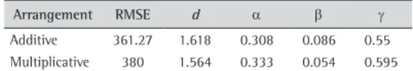
By analyzing the demand’s evolution (Figure 1), we are able to see a trend to go up (the pilling up of the series shows that) and seasonality (valleys and peaks that repeat themselves in all the series, remarkably February’s valley). Considering that both trend and seasonality are present, Holt-Winters’ model becomes the most suitable choice (Section 2.1). In order to choose the model arrangement (additive or multiplicative) and the values of the smoothing constants, we performed tests with both additive and multiplicative arrangements, obtaining RMSE and Durbin-Watson statistic (d) values for both of them (Table 1), the values of the smoothing constants where obtained with mathematical programming. The additive arrangement yielded better results, given its lower value for RMSE and Durbin-Watson statistic closer to 2.
4. Development of a model to Pará’s
IEPS’s biodiesel plant location
The traditional CFLP model is not quite adequate to locate biodiesel plants to supply Pará’s IEPS, mainly because it does not consider the transportation costs the demand will be covered by opened facilities only,
and (19) and (20) keep the variables binary. P-Median assumes that the facility will be able to supply all the demands assigned to it (DAVARIZ, 2006), but this assumption is only true if one knows in advance that the facility will operate below its capacity. To avoid that problem, some models use an upper bound of how much demand one facility can cover (MELKOTE; DASKIN, 2001). Such models are known as Capacitated Facility Location Problems (CFLP) (MIRANDA; GARRIDO, 2004), in which the constraint (16) is relaxed, fixed operating costs are added to (15), and the model is constrained to the facilities’ capacity (MONTEBELLER JÚNIOR; WANKE, 2009). Considering:
• α: transportation cost of one unit of the product, • cj:fixed operating costs the facility located at j, • Wj: capacity of j’s facility.
CFLP is derivate from the P-Median as:
j j k jk jk
j j k
Minimize
∑
c X +α∑∑
h d Y(21)
Subject to:
1 jk j
Y =
∑
(22)0
jk j
Y −X ≤ (23)
k jk j j
k
h Y ≤W X
∑
(24){0,1} j
X ∈ (25)
{0,1} jk
Y ∈ (26)
Equation 21 minimizes the facility-customer transportation costs and the fixed operating costs (assuming that the costs are proportional to the distances). Constraints (22), (23), (25), and (26) act similarly as in the P-Median model, and (24) prevents that more demand is assigned to a facility than its capacity can handle.
3. Modeling Pará’s 2011 biodiesel
demand
For our study, we will consider the 34 IEPS supplied by Pará’s electric power dealer. We will forecast the diesel demand based on Eletrobras (2011) and,
Figure 1. Aggregated demand evolution.
Table 1. Comparison between the arrangements and values of
the smoothing constants.
Arrangement RMSE d α β γ
0
jmk jm
Y −X ≤ (30)
k jmk m jm
k
Hf Y ≤W X
∑
(31){0,1} jm
X ∈ (32)
{0,1} jmk
Y ∈ (33)
The objective function (27) minimizes the annual operating costs of the plants and the total transportation costs. Constraint (28) assures that no more than one facility will be open at a specific location. Constraint (29) determines that all the demand will be covered by a single source. Constraint (30) assures that the demands will be assigned only to opened facilities. Constraint (31) defines the capacity limits of the facilities, and (32) and (33) assure that the variables remain binary.
5. Definition and treatment of input data
For the raw material (palm oil and ethanol), Tailândia and Ulianópolis will be considered as the shipping points, given that these cities are the largest producers, as discussed in Section 1. Another consideration drawn in Section 1 is that, for the sake of balancing the chemical equation, we must consider that: Poil = 0.87 and Pethanol = 0.13. To host biodiesel plants, we chose as candidates cities that have ports. They are: Belém (BRASIL, 2010a), Barcarena (BRASIL, 2010b), Santarém (BRASIL, 2010c), Itaituba (BRASIL, 2010d), Altamira (BRASIL, 2010e), and Marabá (BRASIL, 2010f).
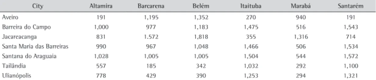
Considering the transportation costs proportional to the distance, one must obtain the distances between the cities and the unitary freight costs (R$/m³.km) to get Sij and Djk. For the arcs ij, we used the road distances from Pará’s Road Map (Table 2) and the freight costs were considered as following: for the palm oil as 0.21 R$/m³.km (Davariz (2006); corrected by Brasil (2011); IGP-M from 01/2006 to 01/2011; considering the oil’s density as 0.91 ton/m³) and to the ethanol as 0.19 R$/m³.km (mean of the values of SIFRECA (SISTEMA..., 2011)).
For the jk arcs, the distances were estimated by two ways: for the IEPS supplied by roads, we used the real distances in Table 2. For the cities supplied by waterways, we estimated it by multiplying the Euclidean distance by a sinuosity factor s. To do that we converted the geodesic coordinates to between the biodiesel plants and the raw material
plants (which is a very important factor in a State with great dimensions like Pará). Also, it is not able to choose among several types of facilities. Other small modification to the model is to include the direct account of the transportation costs instead of using a constant to obtain it.
First, let us add two new indexes to the model: • i: raw materials’ index,
• m: biodiesel plant type’s index.
For our biodiesel case study, the index i indicates palm oil and ethanol, and the index m indicates the plant type. Each plant type has specifics capacity and fixed operating costs.
New parameters also need to be added/modified: • Pi: proportion of the raw material i in the biodiesel
mixture,
• Sij: transportation cost (R$/m³) of the raw material i to the plant at location j (supply cost),
• Cm: annual fixed operating cost (R$) of a plant type
m,
• Wm: annual capacity (m³) of a plant type m, • Djk: transportation cost (R$/m³) of the biodiesel from
j to k (distribution cost),
• H: annual aggregated demand (m³) of biodiesel, • fk: participation of the IEPS k in the aggregated
demand,
The new decision variables are:
• Xjm: opening status of plant type m at j (1 if m is open at k, 0 otherwise),
• Yjmk: covering status of k’s demand by the plant of
type m located at j (1 if k is covered by j’s m plant, 0 otherwise).
The definitions above assert that k jmk
j k m
Hf Y
∑∑∑
isthe total amount of biodiesel needed in the system. We can obtain the biodiesel distribution cost and the raw materials supply cost by multiplying it by Djk and
i ij i
P S
∑
, respectively. Both of these costs sum up into the total transportation cost. Now, we can formulate the following mixed integer programming model:m jm k jmk i ij jk
j m j k m i
Min C X + Hf Y P S +D
∑∑
∑∑∑
∑
(27)
Subject to:
1 jm m
X ≤
∑
(28)1 jmk
j m
Y =
∑∑
results for the optimistic scenario (scenario 1), in which Tocantins and Xingu waterways are navigable. In Section 6.3 we show the current scenario (scenario 2), in which only Tocantins waterway is blocked by Tucuruí Dam. In Section 6.4 we present the scenario of the construction of the Tucuruí Lock, which makes the Tocantins waterway navigable, also the Belo Monte Dam is constructed, what makes Xingu not navigable (scenario 3). The scenario 4 is the pessimist one, with both Xingu and Tocantins not navigable. This scenario is shown in Section 6.5. In Section 6.6 we analyze and comment all the scenarios, focusing on the cost components and the local geography. The mathematical programming problems were solved using an electronic spreadsheet (demand forecast) and the AIMMS software (facility location problems), all the calculations were performed using an AMD Athlon X2 240 processor with 4 GB of RAM memory.
6.1.
IEPS’s demand forecast
First, we forecasted the aggregated diesel demand for 2011. Since we are interested in the Biodiesel demand, the diesel demand was multiplied by a 1.064 factor (discussed in Section 3) to take the diesel/biodiesel loss of efficiency into account. Those results (in m³) are shown in Table 5.
6.2.
Scenario 1: waterways full navegability
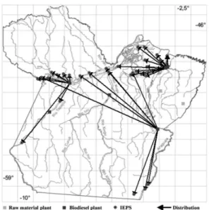
In this scenario, 3 middle-size plants were opened in the cities of Altamira (using 98.85% of the capacity), Cartesian coordinates using Tardelli and Wanke’s
(2009) Equations 34 and 35 (slight modifications to the author’s equations). To calculate s, we compared some actual distances given by Pará (2006) and the corresponding Euclidean distances, which yielded s = 1,31. It must be pointed that we believe that Eletrobras (2011) misclassified Cotijuba’s as road-accessible, given that this IEPS is an island of Belém City. Thus we will consider Cotijuba as waterway-accessible. The geodesic coordinates can be found at Table 3 and in the Appendix A.
(
)
{
}
1
3959 1, 609 cos cos[ ]
x= − × × − rad long (34)
( )
{
}
1
3959 1, 609 cos cos[ ]
y= − × × − rad lat (35)
The unitary road freight cost will be considered as 0.42 R$/m³.km (SISTEMA..., 2011; mean of the values for clear fuels) and the waterway freight will be considered as 0.24 R$/m³.km (58% below the former, as Caixeta-Filho (2001), mentions that waterway transportation is about 58% cheaper than road).
The annual capacity of the biodiesel plants and their annual fixed costs are in Table 4, and were obtained in Carvalho (2008) and corrected by the IGP-M (BRASIL, 2011; 01/2008 to 01/2011).
The total aggregated demand (H) will be shown in Section 6 and is the sum of the demand forecast for 2011. The participation of each IEPS in it (fk) will be considered as 2010’s f (Appendix A).
6. Results and comments
In this Section we present the results of the calculations yielded by the models developed in Sections 3 and 4. In Section 6.1 we show the results of the forecast model. In Section 6.2, we find the
Table 2. Road distances between the road-connected cities.
City Altamira Barcarena Belém Itaituba Marabá Santarém
Aveiro 191 1,195 1,352 270 940 191
Barreira do Campo 1,000 977 1,183 1,475 516 1,543
Jacareacanga 831 1.572 1,818 355 1,316 714
Santa Maria das Barreiras 990 967 1,048 1,466 506 1,534
Santana do Araguaia 1,028 1,005 1,005 1,504 544 1,572
Tailândia 557 185 342 1,032 292 1,100
Ulianópolis 778 429 390 1,253 294 1,321
Table 3. Coordinates of the supply and distribution cities.
Axis Altamira Barcarena Belém Itaituba Marabá Santarém
Lon(°) –3.2 –1.5 –1.45 –4,27 –5.36 –2.44
Lat(°) –52.2 –48.62 –48.5 –55.98 –49.11 –54.7
Table 4. Costs and capacities of the biodiesel plants.
Size Capacity (m³) Cost (R$)
Small 10,989 847,714
Middle 43,956 3,000,218
one small-size plant in Santarém (usage of 96.02%), 1 middle-size plant in Marabá (usage of 28.82%), and 1 large-size plant in Barcarena (usage of 97.37%). The R$ 38,936,354 total annual costs were divided into R$ 11,356,672 of fixed operating costs, R$ 9,402,034 of supply costs, and R$ 18,177,648 of biodiesel distribution costs.
6.6.
Comments on the results
When looking at the total annual costs, one cannot see much of a difference among the scenarios. There is a discrepancy of about 4% between the scenario 1 and 4, which are the ones with the greater and Barcarena (usage of 99.78%), and Marabá (usage of
88.13%) and 1 small-size was opened in Santarém (usage of 96.02%). The total cost was R$ 37,394,907, divided into R$ 9,848,368 of fixed operating costs, R$ 12,017,549 of raw material supply cost, and R$ 15,528,990 of biodiesel distribution cost. The network can be seen in Figure 2.
6.3.
Scenario 2: Tocantins’ navigability
blocked
In this scenario, only 2 plants were opened: one middle-size plant in Altamira (usage of 99.43%) and one large-size in Barcarena (usage of 84.53%). The fixed operating costs were R$ 9,661,244, and the supply and distribution costs were R$ 9,432,082 and R$ 19,041,306, summing a total annual cost of R$ 38,134,632. Figure 3 shows this network.
6.4.
Scenario 3: Xingu’s navigability blocked
The construction of Tucuruí Lock and Belo Monte Dam created the following network (Figure 4): 3 middle-size plants in Barcarena (usage of 99.84%), Marabá (usage of 86.62%), and Santarém (usage of 99.42%) and 1 small-size plant in Belém (usage of 99.54%). The total cost was R$ 38,430,208, of which R$ 9,848,368 were fixed operating costs, R$ 15,254,814 were supply costs, and R$ 13,327,026 were distribution costs.
6.5.
Scenario 4: both waterways not
navigable
The construction of Belo Monte Dam and Tucuruí Dam configured the network as follows (Figure 5): one small-size plant in Itaituba (usage of 58.03%),
Table 5. Biodiesel forecast for 2011 (m³).
Month Forecast
Jan 10,699
Feb 9,93
Mar 10,875
Apr 10,859
May 11,152
June 11,161
July 11,763
Aug 12,198
Sept 11,835
Oct 12,001
Nov 11,844
Dec 12,291
Total 136,608
Figure 2. Network of the scenario 1.
The raw material supply costs changed between the scenarios. Although, a 0.5% resemblance can be seen among the two scenarios with lowest supply costs (2 and 4), both of them differ 34% from the scenario with the highest supply cost (scenario 3) and differ 17% from the supply cost of scenario 4. The low supply costs of scenarios 2 and 4 can be explained by the opening of large-size plants in Barcarena, which is closer to Ulianópolis and Tailândia. The high cost of scenario 3 can be explained by the opening of a middle-size plant in Santarém, in the Northwestern region of the State. So far, Santarém had only received small-size plants, it uniquely supplied the IEPS of Jurutí, that has one of the highest participations in the aggregated demand.
In the distribution costs, we can see that the difference between the highest (scenario 2) and the lower (scenario 3) value is 30%, while the two highest values (scenarios 2 and 4) differ only 5% among themselves, and the two lowest (scenarios 1 and 3) are 14% different. The high values in scenarios 2 and 4 are given to the opening of large-size plants in Barcarena, what forces the centralized demand covering of far away customers. Meanwhile, the low costs of scenarios 1 and 3 can be explained by the decentralization of the demand covering, thanks to the opening the plants closer to the customers.
Despite the differences in the supply and distribution costs, there is some stability in their sum (the transportation cost): R$ 27,546,539 in scenario 1, R$ 28,473,388 in scenario 2, R$ 28,581,840 in scenario 3 and R$ 27,579,682 in scenario 4. This fact allows us to see a trade-off among the transportation costs, and that the difference among the total costs in the scenarios is due to the fixed operating costs.
The analyses allow us to conclude that the navigability of the waterways has a stronger impact in the facilities costs than in the transportation costs, given that the model tends to balance up the latter.
About the local geography, the importance of Barcarena is remarkable. This city is not only close to Ulianópolis and Tailândia, but also close to the demand points that are concentrated in the Northeastern and Northwestern regions of the State. However, Marabá’s importance must also be highlighted: it is the second closer city to the raw material plants, and the closer city to the Southeastern demand points (Santana do Araguaia, Santa Maria das Barreiras, and Barreira do Campo, that are supplied through roads), what allows the covering of these demands with low transportation costs, plus the covering of the demands at the North of the Tocantins waterway. This trade-off is not possible when the Tocantins waterway is blocked by the Tucuruí Dam, so the Northern demands are covered by a plant in either Altamira or Barcarena, and smaller total costs, respectively. Thus, a closer look is
necessary to analyze all the cost components. Scenarios 1 and 3 share the same value for operating costs, which is very close (2% smaller) to the operating cost of scenario 2. However, the fixed cost of the scenario 4 is 15% superior to the latter’s cost, thanks to the opening of plants with low usage (58% of Itaibuba’s plant and 28.82% of Marabá’s plant). The plant in Marabá is opened even though Tocantins waterway is blocked. It supplies by road the cities of Santana do Araguaia, Santa Maria das Barreiras, and Barreira do Campo. As it can be seen, the waterways restriction elevated the costs by busting the economies of scale in the biodiesel plants.
Figure 4. Network of the scenario 3.
by the construction of dams. This fact highlights the impact of the dam construction in the logistics of the region and the need to include locks in the dam’s projects.
Other questions of interest not addressed by this paper would include the improvement of our model to be also able to consider other logistic factors (as inventories). Studies like ours should also be performed with other commodities, to identify key cities and bottlenecks in this commodity network, optimizing the formulation of government projects.
References
BOWERSOX, D.; CLOSS, D.; COOPER, M. Supply chain logistics management. New York: McGraw-Hill, 2002. PMid:12829410.
BRASIL. Banco Central do Brasil. Correção de Valores. Disponível em: <https://www3.bcb.gov.br/CALCIDADAO/ publico/exibirFormCorrecaoValores.do?method=exibirFo rmCorrecaoValores>. Accesso em: 06 fev. 2011. BRASIL. Companhia Docas do Pará. Terminal de Miramar.
Disponível em: <http://www.cdp.com.br/porto. php?nIdPorto=10>. Accesso em: 11 jul. 2010a.
BRASIL. Companhia Docas do Pará. Porto de Vila do Conde. Disponível em: <http://www.cdp.com.br/porto. php?nIdPorto=6>. Accesso em: 11 jul. 2010b.
BRASIL. Companhia Docas do Pará. Porto de Santarém. Disponível em: <http://www.cdp.com.br/porto. php?nIdPorto=3>. Accesso em: 11 jul. 2010c.
BRASIL. Companhia Docas do Pará. Porto de Itaituba. Disponível em: <http://www.cdp.com.br/porto. php?nIdPorto=2>. Accesso em: 11 jul. 2010d.
BRASIL. Companhia Docas do Pará. Porto de Altamira. Disponível em: <http://www.cdp.com.br/porto. php?nIdPorto=4>. Accesso em: 11 jul. 2010e.
BRASIL. Ministério dos Transportes. Secretaria de Política Nacional de Transportes. Porto de Marabá - PA. Disponível em: <http://www.transportes.gov.br/bit/ Terminais_hidro/maraba/pfmaraba.htm>. Accesso em: 01 ago. 2010f.
BROCKWELL, P.; DAVIS, R. Introduction to time series and forecasting. New York: Springer-Verlag, 2002. http:// dx.doi.org/10.1007/b97391
CAIXETA-FILHO, J. Particularidades das modalidades de transportes. In: CAIXETA-FILHO, J.; GAMEIRO, A. (Ed.). Transporte e logística em sistemas agroindustriais. São Paulo: Atlas, 2001.
CARVALHO E. Biodiesel: Análise e dimensionamento da rede logística no Brasil usando programação linear. 2008. Dissertação (Mestrado)-Universidade de São Paulo, São Paulo, 2008.
CONDE, C. Análise de dados e definição de indicadores para a regulamentação de usinas termelétricas dos sistemas isolados. 2006. Tese (Doutorado)-Universidade Federal do Pará, Belém, 2006.
CONDE, C. et al. Regulatory actions due to small thermal plants of isolated systems using telemetering control. IEEE Latin America Transactions, v. 7, n. 2, p. 211-216, 2009. http://dx.doi.org/10.1109/TLA.2009.5256831
the Southeastern demands are covered by Barcarena. When the Xingu waterway is also blocked, a middle size plant is opened in Marabá and, even operating far below its capacity, covers the Southeastern IEPS.
Altamira is another important city in our analysis, it is in an intermediate position between the demands of Northwestern and Western regions and the raw material plants in the Northeastern region. However, if the Xingu waterway is blocked, the city does not receive any plant because the Western IEPS supplied through roads do not have demand enough to compensate the opening of a dedicated plant, as happened with Marabá. Altamira’s importance can be seen in the scenario 2: when the Tocantins waterway is blocked and only two plants are opened, Altamira’s plant covers a good share of the biodiesel demand.
Belém, capital of Pará, has little importance in the scenarios thanks to its proximity (16 km) to Barcarena, which is closer to the Western demands. Santarém, the most distant city from the raw material plants (but closer to the Northwestern demand), appears in two scenarios recieving one plant exclusively to Jurutí and supporting Marabá in the coverage of the Northwestern demands when Altamira does not receive any plant due to the blockage of the Xingu waterway. Itaituba, the second most distant city from the raw materials supply plants, is also relatively distant from the Northwestern demands, in such a way that it only recieves one plant in the worst scenario.
7. Final remarks
The biodiesel demand forecast has been easily obtainable through the diesel demand, needing only an efficiency correction factor. The Holt-Winters’ model returned a low error (RMSE = 361.27), which shows how effective it was to forecast the aggregated demand.
The developed facility location model has been proved to be efficient to consider more factors than the classic CFLP model, given that it was easily modified from the latter. It must be pointed the model’s tendency to level up the transportation costs by trading-off the supply and distribution components, in such a way that our scenarios differentiated themselves mostly in the fixed operating costs.
MIRANDA, P.; GARRIDO, R. Incorporating inventory control decisions into a strategic distribution network design model with stochastic demand. Transportation Research Part E, v. 40, p. 183-207, 2004. http://dx.doi. org/10.1016/j.tre.2003.08.006
MONTEBELLER JÚNIOR, E.; WANKE, P. Teoria e Prática. In: MONTEBELLER JÚNIOR, E.; WANKE, P. (Ed.). Introdução ao planejamento de redes logísticas: aplicações em AIMMS (Optimization Software for Operations Research Applications). São Paulo: Atlas, 2009.
OLIVEIRA, K. et al. Influência da razão molar óleo/etanol na transesterificação do óleo de palma bruto. In: CONGRESSO DA REDE BRASILEIRA DE TECNOLOGIA DO BIODIESEL, 2., 2007, Brasília. Online Procedings... 2007. Disponível em: <http://www.biodiesel.gov.br/ rede_arquivos/rede_publicacoes.htm#II>. Accesso em: 10 out. 2010.
OWEN, S.; DASKIN, M. Strategic facility location: A review. European Journal of Operational Research, v. 111, n. 1, p. 423-447, 1998. http://dx.doi.org/10.1016/S0377-2217(98)00186-6
PARÁ. Portaria nº 261, de 11 de setembro de 2006. Diário Oficial do Estado do Pará, Belém, set. 2006.
SANTOS, A. Análise do potencial do biodiesel de dendê para geração elétrica em sistemas isolados da Amazônia. 2008. Dissertação (Mestrado)-Universidade Federal do Rio de Janeiro, Rio de Janeiro, 2008.
SEGURA, J.; VERCHER, E. A spreadsheet modeling approach to the Holt-Winters optimal forecasting. European Journal of Operational Research, v. 131, p. 375-388, 2001. http://dx.doi.org/10.1016/S0377-2217(00)00062-X SILVA, F. et al. Avaliação do desempenho do motor de
combustão alimentado com diesel e biodiesel. In: CONGRESSO DA REDE BRASILEIRA DE TECNOLOGIA DO BIODIESEL, 1., 2006, Brasília. Online Procedings... Disponível em: <http://www.biodiesel.gov.br/docs/ congressso2006/Outros/AvaliacaoDesempenho8.pdf>. Accesso em: 18 out. 2010.
SISTEMA DE INFORMAÇÕES DE FRETE – SIFRECA. Fretes Rodoviários. Disponível em: <http://sifreca.esalq.usp.br/ sifreca/pt/fretes/rodoviarios/index.php>. Accesso em: 06 fev. 2011.
TARDELLI, R.; WANKE, P. Casos de Ensino. In: WANKE, P.; MONTEBELLER JÚNIOR, E.; TARDELLI, R. (Ed.). Introdução ao planejamento de redes logísticas: aplicações em AIMMS (Optimization Software for Operations Research Applications) São Paulo: Atlas. 2009.
UDAETA, M. et al. Comparação da produção de energia com diesel e biodiesel analisando todos os custos envolvidos. In: ENCONTRO DE ENERGIA NO MEIO RURAL, 5., 2004, Campinas. Online Procedings... Disponível em: <http:// www.proceedings.scielo.br/scielo.php?script=sci_arttext &pid=MSC0000000022004000100039&lng=en&nrm=a bn>. Accesso em: 02 out. 2010.
WANKE, P. Previsão top-down ou bottom-up? Impacto nos níveis de erro e de estoques de segurança. Gestão & Produção, v. 15, n. 2, p. 231-245, 2008. http://dx.doi. org/10.1590/S0104-530X2008000200003
WANKE, P.; SALIBY, E. Top-down or bottom-up forecasting? Pesquisa Operacional, v. 27, n. 3, p. 591-605, 2007. http://dx.doi.org/10.1590/S0101-74382007000300010 WINTERS, P. Forecasting sales by exponentially weighted
moving averages. Management Science, v. 6, p. 324-342, 1960. http://dx.doi.org/10.1287/mnsc.6.3.324
CHOPRA, M.; MEINDL, P. Supply chain management. New York: Pearson Prentice Hall, 2009.
DAVARIZ, R. Procedimento para análise de projeto de rede logística. 2006. Dissertação (Mestrado)-Instituto Militar de Engenharia, Rio de Janeiro, 2006.
DIAS, M. Administração de materiais: princípios, conceitos e gestão. São Paulo: Atlas, 2009.
ELETROBRAS. Programas Mensais de Operação. Disponível em: <http://www.eletrobras.com/ELB/data/Pages/ LUMISB4C86407PTBRIE.htm>. Accesso em: 01 jan. 2011.
FERREIRA, L. Comparação entre as abordagens top-down e bottom-up para previsão de vendas. In: WANKE, P.; JULIANELLI, L. (Ed.). Previsão de vendas: processos organizacionais e métodos quantitativos e qualitativos. São Paulo: Atlas, 2006.
FUNDAÇÃO INSTITUTO DE PESQUISAS ECONÔMICAS - FIPE. Plano estadual de logística e transportes do estado do Pará: análise espacial da agropecuária. São Paulo: FIPE, 2009.
HAKIMI, S. Optimum Locations of Switching Centers and the Absolute Centers and Medians of a Graph. Operations Research, v. 12, n. 13, p. 450-459, 1964. http://dx.doi. org/10.1287/opre.12.3.450
HOLT, C. Forecasting seasonal and trends by exponentially weighted moving averages. Arlington: Office of Naval Research, United States of America, 1957. Research Report 52.
HOLT, C. Forecasting seasonal and trends by exponentially weighted moving averages. International Journal of Forecasting, v. 20, p. 5-10, 2004. http://dx.doi. org/10.1016/j.ijforecast.2003.09.015
INSTITUTO BRASILEIRO DE GEOGRAFIA E ESTATÍSTICA - IBGE. Cidades@. Disponível em: <http:// www.ibge.gov.br/cidadesat/topwindow.htm?1>. Accesso em: 12 set. 2010.
JAYARAMAN, V. Transportation, facility, location and inventory issues in distribution network design: An investigation. International Journal of Operations & Production Management, v. 18, p. 471-494, 1998. http://dx.doi.org/10.1108/01443579810206299
KAHN, K. Revisiting top-down versus bottom-up forecasting. Journal of Business Forecasting, v. 17, n. 2, p. 14-19, 1998.
KOEHLER, A.; SNYDER, R.; ORD, J. Forecasting models and prediction intervals for the multiplicative Holt-Winters method. International Journal of Forecasting, v. 17, p. 269-286, 2001. http://dx.doi.org/10.1016/S0169-2070(01)00081-4
LAPIDE, L. A simple view of top-down versus bottom-up forecasting. The Journal of Business Forecasting, v. 17, n. 2, p. 28-29, 1998.
LAWTON, R. How should additive Holt-Winters estimates be corrected? International Journal of Forecasting, v. 14, p. 393-403, 1998. http://dx.doi.org/10.1016/S0169-2070(98)00040-5
MAKRIDAKIS, S.; WHEELWRIGHT, S.; HYNDMAN, R. Forecasting methods and applications. New York: John Wiley & Sons, 1998.
Appendix A.
IEPS 2006 2007 2008 2009 2010 Coordinates
CVf ρAB CVf ρAB CVf ρAB CVf ρAB CVf ρAB f Lon(°) Lat(°) M
Afuá 7.6% 0.78 5.0% 0.85 7.4% 0.84 7.4% 0.75 3.2% 0.94 1.8% –0.15 –50.38 W
Alenquer 7.4% 0.59 3.6% 0.92 3.8% 0.89 6.9% 0.73 10.2% 0.62 6.4% –1.94 –54.73 W
Almeirín 5.9% 0.71 7.5% 0.58 13.0% 0.30 11.5% 0.73 5.2% 0.84 2.8% –1.52 –52.38 W
Anajás 13.2% 0.42 19.1% 0.61 12.1% 0.75 6.7% 0.80 5.1% 0.93 1.2% –0.98 –49.93 W
Aveiro 12.4% 0.23 19.4% 0.17 11.6% 0.63 36.2% -0.17 17.1% 0.30 0.3% –3.6 –55.33 R
Bagre 5.9% 0.90 11.7% 0.75 14.0% 0.87 13.0% 0.38 4.3% 0.90 0.9% –1.89 –50.16 W B. do Campo 48.3% –0.20 35.5% –0.16 10.5% 0.61 11.7% 0.52 14.7% 0.81 0.2% –9.15 –49.92 R
Breves 5.7% 0.71 6.8% 0.68 7.5% 0.71 9.0% 0.53 5.4% 0.90 9.6% –1.68 –50.47 W
C. do Ararí 10.1% 0.40 8.1% 0.63 4.5% 0.88 5.8% 0.84 5.8% 0.84 1.0% –1.01 –48.96 W
Chaves 43.3% 0.26 18.7% 0.43 22.4% 0.53 17.3% 0.59 17.7% 0.34 0.3% –0.15 –49.98 W
Cotijuba 30.0% –0.16 25.3% 0.52 14.2% 0.48 13.8% 0.53 9.5% 0.69 0.9% –1.24 –48.54 R
Curralinho 6.1% 0.64 8.1% 0.56 14.0% 0.69 7.6% 0.86 4.4% 0.87 1.7% –1.41 –49.79 W Curuá 8.4% 0.60 8.4% 0.63 4.6% 0.90 4.0% 0.92 18.6% 0.1 1.1% –1.88 –55.11 W
Faro 7.2% 0.67 6.0% 0.78 4.5% 0.92 7.5% 0.90 10.5% 0.37 0.9% –2.17 –56.74 W
Gurupá 6.6% 0.60 10.7% 0.41 3.4% 0.94 6.4% 0.86 6.9% 0.82 1.6% –1.4 –51.63 W
Jacareacanga 6.7% 0.60 10.6% 0.24 7.8% 0.72 19.1% 0.41 8.4% 0.94 1.1% –6.22 –57.75 R
Jurutí 20.4% 0.70 10.3% 0.82 15.3% 0.02 37.8% 0.84 3.5% 0.90 7.7% –2.15 –56.09 W
Melgaço 13.6% 0.84 8.8% 0.77 15.9% 0.70 12.9% 0.73 7.9% 0.93 0.8% –1.8 –50.71 W
Monte Alegre 4.2% 0.89 6.3% 0.84 2.9% 0.93 5.7% 0.91 5.5% 0.84 8.5% –2 –54.06 W
Muaná 10.2% 0.34 3.6% 0.93 7.2% 0.85 6.3% 0.81 5.2% 0.86 1.9% –1.52 –49.21 W
Óbidos 5.8% 0.77 8.7% 0.76 5.9% 0.72 10.1% 0.49 5.8% 0.94 6.0% –1.91 –55.51 W
Oeiras do Pará 3.2% 0.90 12.1% 0.42 3.9% 0.90 4.8% 0.89 11.1% 0.64 1.5% –2 –49.85 W Oriximiná 6.1% 0.69 6.1% 0.96 8.2% 0.55 3.5% 0.93 2.8% 0.94 8.5% –1.76 –55.86 W
Ponta de Pedras 4.2% 0.82 4.0% 0.90 8.3% 0.56 7.4% 0.74 5.6% 0.77 2.0% –1.38 –48.87 W
Portel 15.5% 0.11 4.0% 0.94 12.2% 0.33 9.2% 0.64 6.5% 0.87 4.9% –1.93 –50.82 W
Porto de Moz 3.8% 0.92 15.5% –0.29 20.7% -0.4 12.7% 0.78 5.7% 0.90 2.6% –1.74 –52.23 W Prainha 10.1% 0.49 12.6% 0.74 11.1% 0.42 4.2% 0.92 9.0% 0.65 1.5% –1.79 –53.47 W
Salvaterra 5.0% 0.81 5.7% 0.80 6.9% 0.85 8.2% 0.69 4.6% 0.87 4.1% –0.75 –48.51 W
S. C. do Ararí 14.3% 0.68 10.5% 0.87 8.4% 0.76 9.9% 0.66 5.5% 0.96 0.6% –0.66 –49.16 W
S. M. Barreiras 12.2% 0.09 21.1% 0.33 8.1% 0.62 36.6% 0.03 14.6% 0.21 0.4% –8.85 –49.72 R
S. do Araguaia 5.8% 0.64 22.1% 0.64 32.7% 0.43 8.1% 0.64 11.9% 0.17 8.6% –9.5 –50.62 R
S. S. Boa Vista 9.3% 0.61 6.3% 0.90 4.3% 0.87 6.9% 0.77 11.6% 0.72 1.7% –1.71 –49.54 W
Soure 10.6% 0.71 6.0% 0.76 5.5% 0.82 9.7% 0.74 3.5% 0.91 4.3% –0.71 –48.52 W
Terra Santa 9.2% 0.80 6.2% 0.80 3.9% 0.92 5.7% 0.87 5.2% 0.85 2.3% –2.1 –56.48 W
Mean 11.4% 0.58 11.0% 0.63 9.9% 0.66 11.3% 0.68 8.0% 0.73 2.9% - - -