Todos os direitos reservados.
É proibida a reprodução parcial ou integral do conteúdo
deste documento por qualquer meio de distribuição, digital ou
impresso, sem a expressa autorização do
REAP ou de seu autor.
Age-dependent taxes with endogenous human
capital formation
Carlos E. da Costa
Marcelo R. Santos
Carlos E. da Costa
Marcelo R. Santos
Carlos E. da Costa
FGV-EPGE
Praia de Botafogo, 190 - Botafogo, Rio de Janeiro
Marcelo R. Santos
INSPER
formation
∗Carlos E. da Costa
FGV-EPGE
Marcelo R. Santos
INSPER
August 8, 2015
Abstract
We evaluate optimal age-dependent labor income taxes in an environment for which the age-efficiency profile is endogenously determined by human capital investment. The economy is one of overlapping generations in which heterogeneous individuals are exposed to idiosyncratic shocks to their human capital investments, a key element, along with the endogeneity of human capital itself in the determination of optimal age-dependent taxes. Our model is sufficiently rich to study the role of general equilibrium effects, credit market imperfections and different forms of human capital accumulation. The very large welfare gains we find to be generated by age-dependent are lost during the transition to the new steady state if human capital is endogenous. Keywords: Age-dependent taxes; Human Capital AccumulationJ.E.L. codes: E6; H3; J2.
1
Introduction
’Tag’ is how Akerlof [1978] called observable characteristics that agents possess which
should be taken into account in policy design in order to alleviate the distortions caused by
tax-ation. Age, a natural tag recognized inAkerlof’s [1978] original work, has recently drawn
con-siderable attention thanks to a wave of recent contributions on the realm of the New Dynamic
Public Finance (NDPF) literature —Weinzierl[2011],Farhi and Werning[2013], Findeisen
and Sachs[2015].1 The defining feature of the NDPF literature is its reliance on a mechanism
design approach to characterize constrained efficient allocations. This approach has the merit of showing all that is attainable for any given environment. Its main drawback is that char-acterization is often very difficult and important compromises in terms of the richness of the environment are almost always needed.
Inspired byWeinzierl’s [2011] important finding that age-dependent taxes lead to welfare
gains that are very close to those attained at the second best, we focus on age-dependent taxes from the outset. Because we aim not at finding second best allocations, we are able to enrich the environment, and provide a more thorough quantitative assessment of optimal age-dependent
∗Carlos da Costa gratefully acknowledges financial support from CNPq Proc. 307494/2013-6. Marcelo R. Santos
gratefully acknowledges financial support from CNPq Proc. 311437/2014-1. We thank Luis Araujo, Felipe Iachan, Pedro Teles seminar participants at IPEA, FEA-RP, the 2013 REAP, the 2014 LAMES and SBE meetings, the 2015 SED, EEA and Econometric Society meetings, for their invaluable comments. All errors are our sole responsibility.
1Age is free from most of the drawbacks that might have precluded the practical uses of other tags. SeeWeinzierl
[2012] for a discussion of possible reasons for the sub-optimal use of tags in current policies.
taxes.2
A central concern in our assessment is the role played by the assumption that the
age-efficiency profile is invariant to policy.3 The exogeneity of an agent’s productivity along his or
her life-cycle is clearly an inaccurate description of how one’s productivity evolves. Yet, the simplifications allowed for by this assumption is thought to outweigh its costs. This fact is
often explicitly recognized in the literature. Weinzierl[2011], for example, referring to the use
of an exogenous path for wages along the life-cycle, argues that “The specific results of this paper therefore require that a substantial portion of variation of wages with age is inelastic to taxes. A few considerations suggest that this requirement’s effects on the paper’s results may be limited.” The ’exogenous’ effect of the passage of time on the parameters of interest
for optimal taxation is however crucial for the usefulness of age as a tag. In fact, Kapička
[2006,2011],Best and Kleven[2013] introduce human capital formation in aMirrlees’s [1971]
framework and derive policy prescriptions which are the opposite of what Weinzierl [2011],
Farhi and Werning [2013],Findeisen and Sachs[2015] prescribe. While the latter find that
taxes ought to increase with age, the former suggest that they should decrease. Kapička[2006,
2011],Best and Kleven[2013] abstract from idiosyncratic uncertainty, a key element driving
Weinzierl’s [2011],Farhi and Werning’s [2013] andFindeisen and Sachs’s [2013b] results. At a
minimum, the endogeneity of human capital is a force towards weaker dependence than what
is suggested byWeinzierl[2011],Farhi and Werning[2013],Findeisen and Sachs[2015]. But
we cannot a priori discard the possibility that the endogeneity of human capital reverses their result. A careful quantitative assessment is needed.
The economy we study incorporates endogenous human capital formation to a setting which
is essentially that ofConesa et al.[2009]. We assume that age-efficiency profiles are generated
by a Learning-by-doing (LBD) technology of human capital formation and contrast our findings to those of a similar economy with exogenous age-efficiency profile.
We find that marginal tax rates ought to increase with age when human capital is
endoge-nous thus justifying, at least qualitatively, the overall findings ofWeinzierl[2011],Farhi and
Werning[2013],Findeisen and Sachs[2015]. If the age-efficiency profile were exogenous,
opti-mal taxes would be higher at all ages and display more progressivity than what we find when human capital endogeneity is taken into account.
In our main exercise, capital markets are imperfect and taxes are restricted to be positive. We find large welfare gains from a reform that introduces age-dependency on labor income
taxes. When these gains are decomposed using the methodology proposed byHeathcote et al.
[2008] we find that the optimal tax system produces large efficiency gains at the cost of worse risk sharing. Both efficiency gains and risk sharing losses are substantially larger when hu-man capital is endogenous: increased inequality is more tolerable when it is compensated by larger efficiency gains. Another important difference between the two models is that in the LBD model almost all of the gains accrue to the high productivity agents while, with an exogenous age-efficiency profile
The introduction of age dependence reduces the scope for progressivity, when taxes are
2A parallel literature has also emphasized the importance of age-dependent taxes. Starting from the early
contributions ofErosa and Gervais[2002],Garriga[2003] this literature has emphasized the role of capital income taxes and/or progressivity of labor income taxes to mimic age-dependent taxes – see alsoConesa et al.[2009],
Peterman[2011],Gervais[2012],Krueger and Ludwig[2013]. Most of this literature does not take seriously the possibility of using explicit age-dependence, focusing instead on more ’traditional’ instruments. We find these instruments to be poor substitutes for age-dependent taxes, which begs the question: ’why not age-dependent taxes?’
3Very recent works byFindeisen and Sachs[2013a],Stantcheva[2014,2015] have allowed for human capital
restricted to be positive.4 That is, the average and marginal tax rates faced by an agent of any given age vary less with his or her income than it would be the case if he or she were to face
an optimal age-independent schedule.5 Because both taxes and income increase with age, we
might still find more progressivity in the cross-section. This is not however, the case, income taxes are less concentrated in the upper income quantiles than at the benchmark. We also find that the tax system as a whole relies more heavily on labor income taxes than does the benchmark system.
The findings are very different when taxes are allowed to become negative. First, welfare gains are much larger. Indeed an order of magnitude larger than what is found elsewhere. Tax schedules at each age as progressive as the age-independent benchmark schedule. In the cross-section we find that all by the two top quintiles of the income distribution pay negative taxes. Using the welfare decomposition aforementioned, we find some extra efficiency gains from allowing taxes to be negative accompanied by a huge risk sharing improvement. These results regarding possibly unrestricted taxes should be taken with a grain of salt. They are very sensitive to our assumption regarding capital market imperfection.
Another important simplifying assumption adopted in the literature is that of a single co-hort inhabiting a small open economy. We, in contrast, consider a closed overlapping gener-ations economy. We find general equilibrium effects to be important for the distribution of welfare gains. In general equilibrium it is the high ability workers who benefit from the re-form, whereas in partial equilibrium it is low ability one who do. The rationale is easy to grasp. The efficient age-dependent tax system induces a shift of work and after tax income to early years of work. Savings and the stock of capital are increased as a consequence. If prices are allowed to adjust, wages increase and rental rate of capital declines. As labor income becomes more important high ability agents end up benefiting the most from the reform.
In our analysis we compare Steady State allocations, and find very large difference in the capital stock when we compare the optimal with the benchmark tax systems. It is, then, im-portant to ask what the costs for the transition are, a task for which our general equilibrium approach lends itself very naturally. When we take the transition into account, the welfare gains are dissipated when the age-efficiency profile is endogenous, and greatly reduced but not eliminated when it is exogenous.
Finally, we consider the Learning or Doing (LOD) specification for human capital formation
technology due toBecker[1964],Ben Porath[1967].6 With some qualifications, the
endogene-ity of human capital whether under a LBD or a Ben-Porath specification leads to greater re-sponse to policy changes thus making very progressive systems undesirable. As with the LBD model the gains attained in the steady-state induced by the optimal tax system are erased by the transition costs. The most salient difference between the two specifications is that with Ben-Porath human capital formation, the utility impact of allowing taxes to be negative are significantly larger.
A natural question that arises from our assessment is: what are the cost of ignoring the endogeneity of human capital? To address this question we take the schedule derived for the exogenous model and find the equilibrium allocations that arise when the age-efficiency profile is in reality endogenous. We find that about 18% of potential welfare gains are wasted by not taking learning-by-doing into account.
4We use the functional form adopted byHeathcote et al.[2008] both to calibrate the benchmark economy and
to find the optimal progressivity.
5This is in line withFarhi and Werning’s [2013] andWeinzierl’s [2012] findings.
6It is very hard to empirically distinguish which model of human capital formation is more appropriate - see
The rest of the paper is organized as follows. After a brief literature review, Section2 ex-plains the environment as well as the policy instruments available to the Government. The
definition of a recursive equilibrium for the economy is provided in2.5. Details of the
calibra-tion and the planner’s maximizacalibra-tion problem are presented in Seccalibra-tion??. Our main findings
are found in Section4 and we use section5 to address some of the specificities of our model
which make difficult the comparison with the rest of the literature. We find higher welfare
gains than those found elsewhere — Weinzierl[2011],Farhi and Werning[2013], Findeisen
and Sachs[2015] Section 5is intended to investigate potential sources of discrepancies. We
allow agents to borrow against future earnings in section5.2. Holding prices fixed, as we
de-rive optimal taxes, section5.1, we evaluate the contribution of general equilibrium effects to
our findings. Finally in section5.3, we consider an alternative, Ben-Porath specification for
human capital formation. Section6concludes the paper.
Closely Related Literature
After Weinzierl’s [2011] initial contribution, the literature that followed, e.g., Farhi and
Werning [2013], Findeisen and Sachs [2015], Stantcheva [2014], has confirmed his finding
that age-dependence captures the bulk of the gains from history-dependence — see also
Bas-tani et al.[2010]. None of these works include general equilibrium effects or transition costs.
Most have abstracted from human capital formation. Yet,Stantcheva[2014,2015],Findeisen
and Sachs [2013a], Kapička [2006], da Costa and Maestri [2007], Kapička [2011], Kapička
and Neira[2013] do take into account the impact of tax policies on human capital formation.
Kapička[2006,2011] do not allow for idiosyncratic shocks. Stantcheva[2014],Findeisen and
Sachs[2013a],Kapička and Neira[2013],da Costa and Maestri[2007] consider idiosyncratic
shocks but consider very simple settings to focus on the qualitative implications of human
capital endogeneity. Stantcheva[2015] does offer a quantitative assessment, but uses a
spec-ification of human capital for which accumulation takes place by direct monetary investment. Less fundamentally, but just as important, to keep tractability these papers in the NDPF tra-dition focus on very specific preferences and stochastic processes.
More closely related to our work are those which use the overlapping generation structure to connect the optimality of age-dependent taxes to capital income and progressive labor
in-come taxes.7 Gervais[2012], for example, shows that, despite all its efficiency shortcomings,
a progressive labor income tax schedule may be better than a flat tax due to its mimicking
an age-dependent system. Gervais[2012] derives optimal age dependent labor and capital
in-come taxes. He considers neither human capital endogeneity nor idiosyncratic risk. He finds
optimal labor income taxes whichdecreasewith age. Before him, Erosa and Gervais [2002],
Garriga[2003] had already noted that the absence of age-dependent taxes would lead to the
optimality of non-zero capital income taxation since it substitutes, however imperfectly, for the missing age-dependent labor income taxes. Using a representative agent for each cohort, and assuming away any form of uncertainty, they find positive taxes on capital to be optimal in
their setting, a findings are related to marginal tax rates which ought todecreasewith age.
These findings stands in contrast with those inWeinzierl[2011],Farhi and Werning [2013],
Findeisen and Sachs[2015]. A crucial difference is that these latter works is the
redistribu-7A direct application of Ramsey’s formulae —Lucas and Stokey[1983],Chari and Kehoe[1999],Judd[1985] —
tive/insurance provision role of taxes, absent in the former.
Conesa et al. [2009] incorporates both redistribution and insurance concerns to the
Gov-ernment’s objective. Their work addresses many of the central issues that arise in the type of environment we study, which makes it an important reference for our investigation. Their
focus is on capital income taxes, not age-dependent labor income taxes, however.8 As our
quan-titative findings indicate, these instruments are poor substitutes for age-dependent taxes. We take into account elements from this literature in our investigation. The overlapping generations structure separates the time from the age dimensions of policies. Idiosyncratic uncertainty is considered, to capture the insurance role of age-varying policy and we explicitly investigate the role of general equilibrium effects caused by the impact of policies on both human and physical capital accumulation in generating our results. Contrary to them, our
focus is on optimal age-dependent taxes, and we take human capital formation into account.9
2
The Environment
At each point in time, the economy is inhabited by multiple cohorts of individuals of differ-ent ages. Each cohort is comprised of a continuum of measure one of individuals who live for a finite, albeit random, number of periods.
2.1 Demography
Each period, j, a new generation is born. For an individual born in period j, uncertainty
regarding the time of death is captured by the fact that he or she faces a probabilityψt+1 of
surviving to the aget+ 1conditional on being alive at aget. Hence, an individual born injis
alive inj+twith probabilityQt
k=1ψk. We also assume that there isT >0such thatψT+1= 0.
Our focus is on one’s working life, hence an agents life starts at the aget= 16.
For most of our analysis we will focus on the steady-state allocations. Since it greatly
simplifies the presentation we shall drop all time indices from aggregate variables and uset
to represent age.
We may map the survival probability into the time invariant age profile of the population
denoted{µt}Tt=1. Lettinggn denote the population growth rate, the fraction of agents tyears
old in the population is found using the following law of motion
µt= ψt 1 +gn
µt−1,
withµt≥0,PTt=1µt= 1.
2.2 Technology
Technology is standard. The production side of the economy aggregates and the technology for producing the consumption good is summarized by a Cobb-Douglass production function with constant returns to scale,
Y =BKαN1−α,
8Only in Section V.B. do they explicitly discuss the role of age-dependent taxes, and relate the two (p. 41): “...a
positive capital income tax mimics a labor income tax that is falling in age.”
9Krueger and Ludwig[2013] study optimal progressive income taxation when there is endogenous human
whereKis aggregate capital,Nis aggregate efficient units of labor, andBis a scale parameter. Every period, the standing representative firm solves the static optimization problem
max K,N
BKαN1−α−δK−wN−rK ,
where r is the rental rate of physical capital and w is the rental rate of human capital, i.e.
the wage rate. Note that we assume that the rental rate of capital is net of depreciation costs which are born directly by the firm.
The first order conditions for the firm’s profit maximization problem are,
(1−α)BKαN−α=w, (1)
and
αBKα−1N−α−δ=r. (2)
2.3 Households
Preferences Individuals derive utility from consumption,c, and leisure,l.
Preferences defined over random paths of(ct, lt)are represented by the time-separable
von-Neumann Morgenstern utility,
E
" T X
t=1
βt−1
t Y
k=1
ψk !
Ut(ct, lt) #
, (3)
where β is the subjective discount factor, and E is the expectation operator conditional on
information at birth.
We allow preferences over consumption-leisure bundles to vary with age by indexing the
flow utility byt. More spesifically flow utility will be of the form
Ut(ct, lt) =
(ct1−ρtltρt)1−γ−1
1−γ , (4)
forρt∈(0,1)∀t,γ >0,γ 6= 1.
Note that this specification for preferences implies a Frisch elasticity of labor supply which
decreases with hours worked. Indeed, letǫfdenote the Frisch elasticity of labor supply. Then,10
ǫft = (1−γ)(1−ρt)−1
γ
1−nt
nt
.
Elasticities are, of course, crucial in the determination of optimal taxes. So, understanding
how hours vary along the life-cycle will be important in understanding policy prescriptions.11
The fact that we allow the marginal rate of substitution between leisure and consumption to vary with age gives us more degrees of freedom to try to match the behavior of hours along
the life-cycle. As ρ decreases, agents become more willing to forego leisure to obtain more
consumption. Since lowerρ implies higher (in absolute terms) Frisch elasticity of leisure our
the two effects compound to generate more variation in the Frisch elasticity of labor supply.
10The Frisch elasticity is calculated for the model without human capital accumulation. With endogenous human
capital the expressions for Frisch elasticity become much more involved. SeeKeane[2011]
11This property of preferences represented by (4) has played a role in the findings inErosa and Gervais[2002].
Since the data exhibits a pattern of decreasing hours along the life-cycle, Frisch elasticities and optimal taxes
Another issue raised by our choice of time-varying preferences is that for a given n, the marginal utility of consumption varies with age. A perfectly smooth profile would no longer be optimal even if hours were constant. Finally, this choice of preferences requires a different procedure for measuring welfare gains.
Labor Supply and Retirement Every period, individuals choose labor supply,
consump-tion, human capital investment and asset accumulation to maximize their objective, (3), sub-ject to a budget constraint which we shall explain momentarily.
Each person has a unit time endowment which can be directly consumed in the form of
leisure,l, or used in market related activities. An agent’s period-by-period time constraint is
lt+nt = 1. An individual of age t who works for n hours supplies to the market a total of
ntste(u+zt) efficiency units which are paid at a rental ratew. The variableu ∼ N(0, σ2u) is a
permanent component of an individual’s skills. It is realized at birth and retained throughout
one’s life. On the other hand, z evolves stochastically according to an AR(1) process, zt =
ϕzzt−1+εt, with innovationsεt∼N(0, σ2ε).
Whereasuaims at capturing the heterogeneity at birth, everyone’s most relevant lottery,z
is the main source of uncertainty that affects one’s choices. The parameterϕz accommodates
the empirically observed persistence of productivity shocks. stis what we call the age-efficiency
profile, the term which distinguishes the models of human capital we study.
Labor productivity shocks are independent across agents. As a consequence, there is no uncertainty regarding the aggregate labor endowment even though there is uncertainty at the individual level.
Retirement is mandatory at the age of 65, ort= 50.
Human Capital Accumulation At the center of our analysis is the process governing the
age-efficiency profilest. Absent uncertainty,st would be the only term leading individuals to
vary their choices along the life-cycle. It is the assumptions that we make about how st is
determined that will differentiate the three models we present here.
Most of the optimal taxation literature treatsstas exogenous.12 We shall consider a
learning-by-doingtechnology for human capital formation. Individuals accumulate human capital by
working. That is, the law of motion forsis given by
st+1=πsφst ntφn+ (1−δh)st, (5)
where(φs, φn)are parameters that govern both the persistence of the age-efficiency profile and
the impact of hours worked on its evolution.
Asset Accumulation Besides choosing how much leisure to consume individuals trade a
risk free asset which holdings we denoted byat.13
Asset holdings are subject to an exogenous lower bound. More precisely, for our main
ex-ercise, we followConesa et al.[2009] in assuming that agents are not allowed to contract debt
at any age, so that the amount of assets carried over from agettot+ 1is such thatat+1 ≥0.
Because no agent can hold a negative position in assets at any time, we assume without loss
12Notable exceptions areKapička[2011],Peterman[2011],Keane[2011].
13In a learning or doing specification one must also decide how to split the remaining time between work and
that asset takes the form of capital,at=kt, as inAiyagari[1994]. For sake of robustness, we
relax this constraint by allowing some borrowing. 14
Asset accumulation is, of course, an important aspect of life-cycle choices which we aim at capturing here. As we shall make clear, there is exogenous (as well as endogenous) variation in productivity along the life-cycle. Consumption smoothing thus provides a reason for one to accumulate assets. Another aspect of choices is that individuals may resort to self-insurance to protect themselves against the uncertainty on labor income. Savings will be, to some extent, motivated by precautionary reasons.
Budget Constraints To write each agent’s flow budget constraint we need to specify the
fiscal policy that is being used by the Government. In our case, it is important to distinguish the current fiscal policy, needed to calibrate the model, from the ones we evaluate. The current tax system will be the benchmark for our studies.
2.4 The Government
The Benchmark Tax System The government levies taxes on capital income, consumption,
and labor income. We assume that consumption is taxed at a rateτc and capital income at a
rate τk. The government also runs a social security system with contributions and benefits
that are equal in equilibrium.
Tax revenues are raised to finance an exogenous flow of expenditures,G.
We approximate the benchmark labor income tax with a tax schedule of the formT(y) =
min
y−ξ0y1−̺; 0 , whereξ0, ̺∈R.
Note that total tax are restricted not to exceed one’s income, i.e.,y > y−ξ0y1−̺, orξ0 >0,
and marginal tax cannot exceed100%, i.e.,T′(y) = 1−ξ
0(1−̺)y−̺<1, orξ0(1−̺)>0.
We approximate the current system with one for which benefits are independent of
contri-butions. Contributions are of the formTss(y) =τssmin{y, ymax}, whereymaxis the contribution
ceiling, and benefits are a fractionθof average income. We choose the parameters to guarantee
that the social security budget is always balanced.
Note, however, that under this specification for the social security important allocative effects remain. First, for many poorer or unlucky agents such social security scheme reduces the incentives to accumulate wealth and, in fact, to run assets down as retirements approaches. Also, with regards to labor supply distortions, the contribution structure is clearly regressive. The overall progressivity of the system should be taken into account when one evaluates the tax prescriptions we derive.
We finally assume that the government collects the accidental bequests and transfers to all agents in the economy on a lump-sum basis.
Optimal Systems We search for the optimal systems within a restricted class. That is our
candidate optimal systems are comprised of an age-dependent labor income tax of the form
Tt(y) = miny−ξty1−̺; 0
where ξtis the parameter that we allow to depend on age, an age-independent consumption
taxτc, and an age-independent capital income taxτk.
14The maximum amount of borrowing allowed is chosen to match the current level of indebtedness observed in
The restriction on consumption taxes is natural if we accept that taxes on consumption are anonymous. This is a reasonable assumption for the majority of goods due to negligible transaction costs. As for capital income taxation, one may argue that most savings are not anonymous since they require the existence of institutions that guarantee the enforcement of contracts. Therefore, we think of age independence as a true arbitrary restriction on taxes which we impose to focus on our main question.
The parameter ̺ aims at capturing progressivity in the tax schedule. There is no single
definition of progressivity. One possibility is to require marginal tax rates to be increasing,
which requires̺(1−̺)ξt>0, or average marginal tax rates to be increasing, which requires,
̺ξt>0.15 Due to the computational costs involved, we restrictξtto be such thatξt= (ξ0−ξ1t),
withξ0, ξ1 ∈R. Hence, taxes are increasing (resp. decreasing) in age ifξ1 >0(resp. ξ1 <0).
In our baseline evaluation we have restricted total taxes to be non-negative. By removing this restriction we endow the Government with a very powerful instrument for redistributing income and relaxing the borrowing constraints. We have also calculated the optima for the unrestricted instruments, and display all our findings for comparison.
Recursive Formulation of Households’ Problem
The flow budget constraint that individuals face in our model economy is, therefore,
kt+1+ (1 +τc)ct= [1 +r(1−τk)]kt+yt−Tt(yt)−Tss(yt) +ǫ∀t, (6)
fort≤T.
By assumptiona1 = 0. Moreover, given that there is no altruistic bequest motive and death
is certain at the ageT+1,agents who survive until ageTconsume all their available resources.
That is,aT+1 = 0, and
cT =
[1 +r(1−τk)]kT−1+ǫ
1 +τc
. (7)
In both (6) and (7),ǫis a lump sum transfer related to the involuntary bequests left by those
who die before reaching ageT + 1. Note that ǫis not age-dependent, i.e., we assume that the
lump sum transfer is identical across cohorts. Moreover, since in a steady-state time and age
can be treated identically,ǫneed not be indexed.
LetVt(ωt)denote the value function of an individual agedt < T+1, whereωt= (at, u, zt, st)∈
Ωis the individual state. In addition, considering that agents die for sure at ageT and that
there is no altruistic link across generations, we have that VT+1(ωT+1) = 0. Thus, the
op-timization problem of individuals agedtunder the exogenous productivity path problem and
the leaning-by-doing economies can be recursively represented as follows. Letω′= (a′, u, z′, s′),
then,
Vt(ω) = max n,a′≥0:
Ut(c,1−n) +βψt+1Ez′Vt+1(ω′)
, (8)
subject to (6), in the case of the exogenous productivity path economy, and to(6) and (5), in
the case of the learning by doing economy.
The same problem under the learning-or-doing approach is given by:
Vt(ω) = max n,e,a′≥0:
Ut(c,1−n−e) +βψt+1Ez′Vt+1(ω′)
(9)
15Alternatively, note that
T′
t(y)
Tt(y)/y
= 1−(1−̺)ξty
−̺
1−ξty−̺
subject to(6)and(10)whereω′= (a′, u, z′, s′).
It should be stressed that we have imposed non-negativity constraints on asset holdings. We have thus taken an extreme (albeit plausible) position with regards to capital markets. Relaxing a little the assumption by allowing some exogenous limit is likely to have little effect on our conclusions, at the cost of introducing a whole new set of issues that would have to be dealt with to maintain the internal consistency of the model.
Also important is the fact that we have only used individual state variables in ω. It is
apparent that prices do enter the value function. Indeed, in solving the model we will need to find the equilibrium prices by explicitly taking into account how they enter the policy functions associated with (8).
2.5 Recursive competitive equilibrium
In all that follows we describe the recursive equilibrium in a steady state. This greatly simplifies the presentation. Moreover it dispenses with the distinction between age and time thus significantly reducing the notational burden.
At each point in time, agents differ from one another with respect to age t and to state
ω = (a, u, z, s) ∈ Ω. Agents of age t identified by their individual states ω, are distributed
according to a probability measure λt defined on Ω, as follows. Let (Ω,̥(Ω), λt) be a space
of probability, where̥(Ω)is the Borelσ-algebra onΩ: for eachη ⊂ ̥(Ω),λt(η) denotes the
fraction of agents agedtthat are inη.
Given the agetdistribution,λt,Qt(ω, η)induces the aget+ 1distributionλt+1 as follows.
The function Qt(ω, η) determines the probability of an agent at age t and stateω to transit
to the setη at aget+ 1. Qt(ω, η), in turn, depends on the policy functions in (8), and on the
exogenous stochastic process forz.
A recursive competitive equilibrium for the economy with human capital accumulation based on learning-by-doing is as follows.
Definition 1. Given the policy parameters, a recursive competitive equilibriumfor the
exogenous path and the learning-by-by doing economies are a collection of value functions
{Vt(ω)},policy functions for individual asset holdingsda,t(ω),for consumptiondc,t(ω),for
la-bor supplydnw,t(ω), prices{w, r}, age dependent but time-invariant measures of agentsλt(ω),
transfersǫand a tax on consumptionτcsuch that:
(i) {da,t(ω), dnw,t(ω), dc,t(ω)}solve the dynamic problems in (8);
(ii) individual and aggregate behaviors are consistent, that is:
K= T X
t=1
µt ˆ
Ω
da,t(ω)dλt
N = T X
t=1
µt ˆ
Ω
dnw,t(ω)st(ω) exp(u+zt)dλt
C= T X
t=1
µt ˆ
Ω
{dc,t(ω)}dλt;
(iv) The final good market clears:
C+G+δK=KαN1−α;
(v) given the decision rules,λt(ω)follows the law of motion:
λt+1(η) =
ˆ
Ω
Qt(ω, η)dλt ∀η⊂̥(Ω);
(vi) the distribution of accidental bequests is:
ǫ= T X
t=1
µt ˆ
Ω
(1−ψt+1)da,t(ω)dλt
(vii) taxes are such that the government’s budget constraint,
τcC+τkrK+ T X
t=1
µt ˆ
Ω
Tt(dnw,t(ω)st(ω) exp(u+zt))dλt=G,
and
PT t=1µt
ˆ
Ω
Tss(dnw,t(ω)st(ω) exp(u+zt))dλt
MT ˆ
Ω
dnw,t(ω)st(ω) exp(u+zt)dλt
=θ
are satisfied every period.
Note also that item (vii) is redundant if conditions (i)–(vi) hold.
2.6 The Planner’s Program
The planner’s objective requires some discussion. For any Paretian objective, the planner must maximize a non-decreasing function of agents’ expected utilities.
There are two relevant questions to be answered. First is how to weight different agents of the same cohort. Second, how to weight the different cohorts.
For the first question, we assume that the Planner chooses policy parameters in order to maximize a Utilitarian social welfare function. That is, the government weights equally all individuals of the same cohort.
As for the second, what we do in practice is to followConesa et al.[2009] in assuming that
the government maximizes the ex-ante lifetime utility of an agent born into the stationary equilibrium implied by the optimal policy.
3
Calibration
The population age profile{µt}Tt=1 depends on the population growth rate,gn, the survival
probabilities,ψt, and the maximum age,T, that an agent can live. Agents enter the economy
at age 16 and live for 75 years,T = 75, so that the real maximum age is 90 years.
Data on survival probability by age were extracted fromBell and Miller[2005]. Given the
survival probabilities, the population growth rate is chosen so that the age distribution in the
model replicates the dependency ratio observed in the data. By settinggn= 0.0105, the model
generates a dependency ratio of 17.27%, which is close to the dependency ratio observed in the data for 2000.
To calibrate the preference parameters we proceed as follows. First, we choose the discount
factorβin such a way that the equilibrium of our benchmark economy implies a capital-output
ratio around of3.0, which is the value observed in the data. Then we fix the parameterγ to
4.0, from micro evidence, and choose the share of leisure in the utility function, ρt, to match
average ours for different age groups. In particular, we assume thatρt=ρ0+ρ1t. To calibrate
ρ0, we use the average working hours for ages19−40and forρ1 the average between41−60.
The first group works on average37.86 while the second40.37 of their time endowment. For
the last5 years we specify a new profileρt = ρ60+ρ2t. We calibrateρ2 to match the average
hours during those last five years equal to35.16.16
The parameters that characterized the stochastic component of individuals productivity
are(σ2u, ϕz, σ2ǫ). Several authors have estimated similar stochastic process for labor
produc-tivity. Controlling for the presence of measurement errors and/or effects of some observable
characteristics such as education and age, the literature provides a range of[0.88,0.96]forϕz
and of [0.10,0.25] for σǫ2. In this article, we rely on the estimates of Kaplan [2012], setting
ϕz = 0.94 andσǫ2 = 0.016. Then, the parameterσu2 was chosen in order for the Gini index for
labor income in the model to match its counterpart in the data, which is nearly 0.43. The value
obtained forσ2u is in line with the estimates in Kaplan[2012] who provides a point estimate
of 0.056 for this parameter. We discretize the two shocks in order to solve the model, using three states to represent the permanent shock and seven states for the persistent shock. For expositional convenience, we refer to the two extremes of the grid for the permanent shock as low and high ability.
The values of technological parameters(α, δ)are also summarized in1. We chose a value
forαbased on U.S. time series data from the National Income and Product Accounts (NIPA).
The depreciation rate, in turn, is obtained byδ = K/YI/Y −g.We set the investment-product ratio
I/Y equal to0.25and the capital-product ratioK/Y equal to 3.0. The economic growth rate,
g,is constant and consistent with the average growth rate of GDP over the second half of the
last century. Based on data from Penn-World Table, we set g equal to 2.7%, which yields a
depreciation rate of5.4%.
The age-efficiency profile for the exogenous model is set to be consistent with the values
estimated in Kaplan [2012], which are based on the average hourly earnings by age in the
PSID. We use a second order polynomial to smooth this profile and extend it to cover ages from
16to65.
In order to calibrate the parameters of the skill accumulation functions, we first set δh =
0.05, which is consistent with the evidence presented inHeckman et al. [2002] who suggest
a range of [0.0016,0.089] for this parameter. In the LBD case, we follow Chang et al. [2002]
who use PSID data set to estimate this equation. In particular, we use their posterior point
estimates ofφs,LBD = 0.40 and φn = 0.35. In the case of LOD parameters, Heckman et al.
[1998] show that the ratio of time spent on training to market hours starts at about40% at
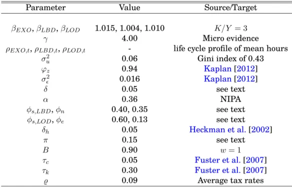
Table 1: Parameter Values - Baseline Calibration
Parameter Value Source/Target
βEXO,βLBD,βLOD 1.015, 1.004, 1.010 K/Y = 3
γ 4.00 Micro evidence
ρEXO,t,ρLBD,t,ρLOD,t - life cycle profile of mean hours
σ2
u 0.06 Gini index of 0.43
ϕz 0.94 Kaplan[2012]
σ2ǫ 0.016 Kaplan[2012]
δ 0.05 see text
α 0.36 NIPA
φs,LBD,φn 0.40, 0.35 see text
φs,LOD,φe 0.60, 0.13 see text
δh 0.05 Heckman et al.[2002]
π 0.15 see text
B 0.90 w= 1
τc 0.05 Fuster et al.[2007]
τk 0.30 Fuster et al.[2007]
̺ 0.09 Average tax rates
ages 20−22 and then declines to near zero by age 45. In addition, the ratio between the
average time spent on training over the life-cycle and market hours is about 6%. Thus, by
choosingφs,LBD= 0.60andφe = 0.10, our model is able to reproduce these calibration targets
in the benchmark economy. We then calibrate the scale parameterπ in order to match the
average growth rate of the age-efficiency profile observed in the data, which is nearly2.3%.
This procedure generates age-efficiency profiles in the human capital models that are close to the one calibrated in the exogenous model.
Finally, we specify the others parameters related to government activity. First, we set
government consumption,G, to18%of the output of the economy under the baseline
calibra-tion. Following the literature, we assume a consumption tax of6%and a capital income tax
rate of30%.17 The parameter̺, which governs the progressivity of the labor income taxes, is
calibrated to match the actual average tax rates. Marginal tax rates at the benchmark are
age-independent,ξ1 = 0, and chosen to raise enough revenue to finance government consumption.
The value we find forξ0 vary slightly across models, but stands between23%and23.5%.
As for Social Security, contributions are of the form Tss(y) =τssmin{y, ymax}, where ymax
is the contribution ceiling. Benefits are a fractionθof the economy’s average income,ym. The
parameter θ was chosen as follows. First, since in the data, ymax = 2.30ym, this is how we
pickymax. Then,θ is chosen in such a way that, at balanced budgetτss ≈ 6.20%. Using this
procedure we getθ=.35which is close to the values typically used in the literature.
Figure1compares the allocations induced by the benchmark tax system for both the
exoge-nous specification of age-efficiency profile and the LBD models. The top left graphs displays the age-efficiency profile for each of model, whereas the graph in the left displays the cor-responding hours. The three figures in the bottom show how taxes vary with income, how consumption and assets accumulation change with age.
Averages may, of course, hide a rich diversity in life-cycle patterns. We split the individuals in our economy in three different ability groups. We group the agents in the high extreme of
the grid of the distribution of innate ability, u, and label them the high ability group. The
agents on the lowest extreme of the grid are labeled low ability. In Figure4, we plot the same
variables considered in Figure3for each of these groups along with the overall average to get
a sense of how heterogeneity plays in our model.
Life-cycle patterns are qualitatively similar for all groups and all models. High ability individuals do, however, work more hours and accumulate more assets than lower ability in-dividuals for all different specifications of human capital dynamics. The age-efficiency profile exhibits some differences across the models. For the exogenous model, we assume that they do not vary across abilities. For the other two models the high ability individuals display a more pronounced increase in productivity, even though this is barely noticeable for the
Learning-or-doing model.18
4
Results
We split the presentation of our results in four parts. First, we discuss our findings
regard-ing optimal taxes. Second, we show how these taxes affect aggregate variables like output,Y,
capital income ratioK/Y, wages, etc. Third we discuss the distributive consequences of our tax
reform. Finally we consider the costs of transition and the costs of ignoring the homogeneity of human capital.
Our main results regarding the tax reform we propose are summarized in Tables2to8. We
shall present them as follows. We first, describe the restricted (to be positive) and unrestricted optimal tax schedules derived under the two different specifications for human capital accu-mulation. Then we show how these schedules affect aggregate variables. Finally, we show how restricted and unrestricted taxes differ substantially with respect to their distributive consequences.
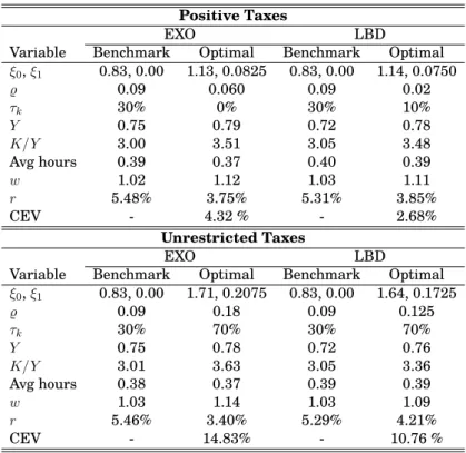
Table 2displays benchmark and optimal policy findings for both the LBD and the
exoge-nous models concerning: i)the tax system,ξ0, ξ1, ̺andτk;ii)equilibrium prices,wandr;iii)
equilibrium aggregate variablesY,K/Y and average hours, andiv)welfare gains, CEV. For
the top panel, labor income, taxes are restricted to be positive, both at the benchmark and at
the optimum, whereas in the bottom panel, both can take negative values.19
4.1 Taxes
The main feature of our reform is the introduction of age-dependence in labor income taxes. We considered two different possibilities for optimal taxes. In our main exercises we restricted taxes to be positive therefore ruling out direct transfers from the government. We, then, re-moved this positivity restriction to explore the value of using labor income taxes as an instru-ment for redistribution/insurance and the relaxation of borrowing constraints. We optimized with respect to capital income taxes, as well, in all our exercises. They too have important allocative consequences which matter for welfare analysis.
Before we describe our main results it is important to emphasize some of the limitations
imposed by the functional form that we have adopted,Tt(y) = y−ξty1−̺. First note that we
needξt >0for taxes to remain below 100%. On the other hand, progressivity in the sense on
18When we compare the cross-sectional distribution of income generated by the model, Table4— with what we
find in the data, e.g. DeNavas-Walt et al.[2013], we find a remarkable adherence. When it comes to assets the model does not do as well, which is not surprising given the well known difficulties of generating the empirical distribution of wealth using well fitted stochastic labor income processes.
19Note that ’total’ taxes are constrained to be non-negative for all agents in the top panel. We are not imposing
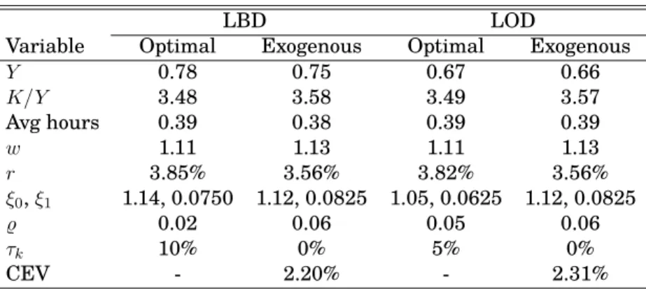
Table 2:Optimum with age-dependent taxation: LBD vs EXO.The table displays the values for the relevant
variables – GDP (Y), capital-output ratio (K/Y), average hours (Avg hours), wages (w), real interest rates(r), policy parameters (ξ0, ξ1, ̺) and welfare (Welfare and CEV)– for both models of human capital formation, Exogenous
(EXO) and Learning-by-doing (LBD) for the benchmark and the optimum.
Positive Taxes
EXO LBD
Variable Benchmark Optimal Benchmark Optimal
ξ0,ξ1 0.83, 0.00 1.13, 0.0825 0.83, 0.00 1.14, 0.0750
̺ 0.09 0.060 0.09 0.02
τk 30% 0% 30% 10%
Y 0.75 0.79 0.72 0.78
K/Y 3.00 3.51 3.05 3.48
Avg hours 0.39 0.37 0.40 0.39
w 1.02 1.12 1.03 1.11
r 5.48% 3.75% 5.31% 3.85%
CEV - 4.32 % - 2.68%
Unrestricted Taxes
EXO LBD
Variable Benchmark Optimal Benchmark Optimal
ξ0,ξ1 0.83, 0.00 1.71, 0.2075 0.83, 0.00 1.64, 0.1725
̺ 0.09 0.18 0.09 0.125
τk 30% 70% 30% 70%
Y 0.75 0.78 0.72 0.76
K/Y 3.01 3.63 3.05 3.36
Avg hours 0.38 0.37 0.39 0.39
w 1.03 1.14 1.03 1.09
r 5.46% 3.40% 5.29% 4.21% CEV - 14.83% - 10.76 %
increasing average tax rates, requires̺ >0. This allows the planner aims to make transfers for
low income agents but not for high income agents it we do not restrict taxes to be non-negative.
Anyone with income y < ξt1/̺ will receive net transfers, while those with income above this
value will pay positive taxes in this case. Note that this implies increasing marginal tax rates.
Hence, subsidies for the poor with decreasing marginal tax rates, prescribed inFindeisen and
Sachs[2015], for instance, cannot be reproduced here.
Restricted Taxes The top panel in table 2displays the main results regarding restricted
taxes. The first three lines contain the results concerning the tax system.
The first thing to note is that for all our specifications taxes are increasing in age, i.e.,ξ1>0.
The number is greater for the exogenous specification of human capital, indicating that taxes should respond to age more in this case than in the LBD specification. As for progressivity,
average and marginal tax rates are increasing in income at all ages: ̺ξty−(̺+1) >0, and̺(1−
̺)ξty−̺−1 >0, respectively.
Figure5provides a very graphic description of optimal labor income taxes. All figures in the
top refer to restricted taxes. The two panels in the left display optimal average and marginal tax rates for the LBD model for the ages 20, 40 and 60. As already stated, taxes increase in age. To get a better grasp about progressivity, we display in green the calibrated benchmark tax schedule and in a blue continuous line the optimal age independent labor income tax sched-ule. When we compare the progressivity, conditional on age, of optimal schedules with the benchmark, if anything, the current system is too progressive. It is also apparent that if tax schedules could not be age dependent, than the optimal schedule would be significantly more
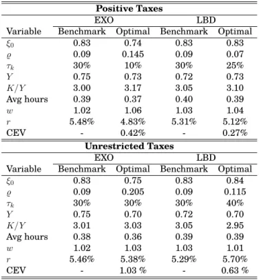
progressive than the current one — see table3. The panels in the right compare taxes for the
Table 3:Optimum with age-independent taxation: LBD vs EXO.The table displays the values for the relevant
variables – GDP (Y), capital-output ratio (K/Y), average hours (Avg hours), wages (w), real interest rates(r), policy parameters (ξ0, ̺) and welfare (CEV)– for both of human capital formation, Exogenous (EXO) and
Learning-by-doing (LBD) for the benchmark and the optimum.
Positive Taxes
EXO LBD
Variable Benchmark Optimal Benchmark Optimal
ξ0 0.83 0.74 0.83 0.83
̺ 0.09 0.145 0.09 0.07
τk 30% 10% 30% 25%
Y 0.75 0.73 0.72 0.73
K/Y 3.00 3.17 3.05 3.10
Avg hours 0.39 0.37 0.40 0.39
w 1.02 1.06 1.03 1.04
r 5.48% 4.83% 5.31% 5.12%
CEV - 0.42% - 0.27%
Unrestricted Taxes
EXO LBD
Variable Benchmark Optimal Benchmark Optimal
ξ0 0.83 0.75 0.83 0.84
̺ 0.09 0.205 0.09 0.115
τk 30% 30% 30% 40%
Y 0.75 0.70 0.72 0.70
K/Y 3.01 3.03 3.05 2.95
Avg hours 0.38 0.36 0.39 0.39
w 1.02 1.03 1.03 1.01
r 5.46% 5.38% 5.29% 5.70% CEV - 1.03 % - 0.63 %
age, when the age efficiency profile is exogenous.
Note also how remarkably similar the optimal age-independent tax is to the benchmark schedule in the LBD model. This is true not only for the labor income tax but also for the capital income tax.
Allowing taxes to depend on age reduces the need for progressivity, conditional on age. This explains why the optimal age-independent schedule is more progressive than schedules for all
ages that we consider. Figure 5 makes this very clear. Indeed, because both labor income
and taxes increase in age it is plausible that progressivity is higher in the cross-section, even
if it is not conditional on age. Eyeball examination of Figure 5 suggests that this is not the
case, a perception reinforced by the numbers displayed in Table4 where effective taxes are
shown to increase less in earning than at the benchmark. Indeed, ff we focus on taxes paid by the 10% richest agents, it decreases from 47.4% of total taxes in the benchmark to 40.3% at the optimum in the LBD model, despite the fact that labor earning slightly increase for this
group from 31.6% to 32.2% — Table4. The equivalent figures for the exogenous model are,
respectively, 45.7% and 44.3% for taxes and 30.7% and 31.0% for earnings.
Finally, at the optimum, capital income taxes become much less important. The marginal tax rate reduces to 10% in the LBD and 0% in the exogenous model. Revenues from capital
income taxation also play a lesser role when we move to the optimum. From Figure 5, it is
apparent that taxes are higher at all income levels. The planner relies more on labor income
taxes, which participation in total government revenue raises from 55% to 73% — Table 5
Table 4: Income, Wealth and Taxes: LBDThe table displays the percentage of labor income earned, labor
income taxes paid and wealth by quantile of each distribution.
Income and Wealth Distribution: Benchmark
20% 20%-40% 40%-60% 60%-80% 80%-100% 90%-100%
Labor Income 4.18 8.72 14.52 23.44 49.15 31.57 Taxes 0.02 2.41 8.81 21.26 67.50 47.37 Assets 1.44 5.28 11.39 23.10 58.78 31.57
Income and Wealth Distribution: Optimum
20% 20%-40% 40%-60% 60%-80% 80%-100% 90%-100%
Labor Income 3.54 8.39 14.26 23.71 50.11 32.19 Taxes 1.37 4.68 10.87 23.17 59.91 40.34 Assets 1.53 5.44 11.72 23.27 58.04 32.19
Income and Wealth Distribution: Benchmark (neg. taxes)
20% 20%-40% 40%-60% 60%-80% 80%-100% 90%-100%
Labor Income 4.02 8.67 14.52 23.44 49.25 31.68 Taxes -0.87 2.37 8.85 21.44 68.21 47.87 Assets 1.58 5.31 11.35 23.04 58.73 38.29
Income and Wealth Distribution: Optimum (neg. taxes)
20% 20%-40% 40%-60% 60%-80% 80%-100% 90%-100%
Labor Income 4.17 8.72 14.34 23.52 49.25 31.49 Taxes -71.85 -74.41 -54.75 6.07 294.95 237.55 Assets 1.95 6.25 13.06 23.97 54.45 34.66
taxes can also be useful for redistribution, in which case one would want some agents to be subsidized thus leading to less reliance on labor income taxes. We have shut this channel down in our main policy experiment. We shall see how these results change when we consider unrestricted taxes, momentarily.
Unrestricted Taxes If taxes are allowed to turn negative, the results change quite
dramat-ically — see bottom panel of table2. Labor income taxes are still increasing in age, but this
is about all that is similar. First, progressivity, even when conditioned on age, increase with respect to the benchmark. When this is combined with the fact that income and taxes increase in age, the resulting impact on the degree of progressivity of the tax system is dramatic.
For the first three quintiles of the income distribution labor income taxes are negative,
i.e., most agents are entitled to transfers as one can see in table4. Labor income taxes are
Table 5:Revenue Distribution: LBD vs EXO.The table displays the fraction of total Government revenue raised
from each tax base: labor income, capital income and consumption at the benchmark, the optimal age-dependent, the optimal age-independent and the optimal age-dependent taxes in Partial Equilibrium.
EXO
Benchmark Optimal
Tax Base Age-dep. Age-indep. Age-dep - PE Labor Income 54.99 81.84 75.02 82.00 Capital Income 27.32 0.00 8.29 0.00 Consumption 17.69 18.16 16.69 18.00
LBD
Benchmark Optimal
Table 6: Revenue Distribution: LBD vs EXO. Negative TaxesThe table displays the fraction of total
Gov-ernment revenue raised from each tax base: labor income, capital income and consumption at the benchmark, the optimal age-dependent, the optimal age-independent and the optimal with prices held constant.
EXO
Benchmark Optimal Tax Base Age-dep. Age-indep. Labor Income 54.96 32.33 58.52 Capital Income 27.33 50.42 25.31 Consumption 17.71 17.25 16.17
LBD
Benchmark Optimal Tax Base Age-dep. Age-indep. Labor Income 55.35 29.93 46.03 Capital Income 26.93 58.35 36.59 Consumption 17.72 18.19 17.38
almost entirely collected from the top 20 or even 10% richest agents. This must however be tempered by the fact that the planner relies less on labor income taxes and more on capital
income taxes for the purpose of raising revenue — see bottom panels of Figure5. The share
of total revenues raised through labor income taxes decreases from 55.4% to 29.9% in LBD model and from 55.0% to 32.3% in the exogenous model. That is, labor income taxes become less important at the same time that they are made significantly more progressive.
Note that in all cases, taxes are higher and more progressive for the exogenous model than for the LBD model. The age-efficiency profile endogeneity is an extra margin where behavioral responses add to the costs of taxation. This must be taken into account in the design of optimal tax systems.
All in all, what we observe is a contrasting use of taxes depending on whether net transfers are possible or not. When taxes are restricted to be positive, the greater efficiency attained by age-dependence is used to increase the reliance on labor income to raise revenue. When taxes are unrestricted, labor income taxes become a powerful instrument for redistributive or insurance provision purposes. The planner exploits this instrument as much as possible,
thus leaving to capital income taxes a more significant role for revenue collection —6. The
consequences of these contrasting results is what we explore until the end of this section. Before, however, a discussion of capital income taxes is due.
Capital income taxes play many different roles in our setting. Beyond the obvious fact that capital income is an important tax base, capital income taxes are useful for redistribu-tive and insurance purposes. Agents with higher labor temporary or permanent labor income save more in absolute terms. As a consequence, taxes on capital income help promote redis-tribution. Second, accumulated wealth dampens work incentives. By taxing capital income, the planner reduces this effect. Third, because there is uncertainty regarding future income, agents may over-accumulate wealth for precautionary reasons. If this is effectively taking place, capital income taxes and a pay-as-you-go Social Security system may be used to reduce
this inefficiency. 20 Finally, a subtle issue that arises in this economy is related to the
ex-ternalities identified ind’Ávila et al.[2012]. Increased capital accumulation leads to changes
in relative prices of labor and capital, increasing the former relative to the latter. As a
con-20Agents cannot borrow in our model, which is a key element in an environment where we expect precautionary
sequence, a larger fraction of one’s income is risky, with no markets to insure against labor income shocks. Capital income taxation may act as a Pigouvian tax in this case.
Allowing taxes to depend on age, greatly increases their efficiency: the same revenue can be raised at the lower welfare cost. When taxes are restricted to be non-negative, this efficiency gain leads to more reliance on labor income taxes, and capital income taxes are reduced.
Our results therefore indicate that the redistributive role can be more efficiently performed by the age-dependent tax or even a more progressive age-independent labor income tax. More-over, given the age efficiency profiles’ steepness along with the existence of a pay-as-you go social security system it is unclear whether agents are over-saving. In fact, it is possible to check that for some agents the borrowing constraint is binding, instead. I.e., they are eager to dis-save at the optimum. This reduces the scope for capital income taxation. Similarly, with-out the possibility of making transfers to agents, the role for redistribution is limited. As for
the externalities, we assess whether it is quantitatively important in Section5.1, where we
consider optimal taxes in a Partial Equilibrium setting. For now, it is enough to mention that, although we do find some role for capital income taxation, it does not seem to be quantitatively important.
The final result is that the optimal tax rate on capital income decreases from 30% to 5% in the LBD model and to 0% for the exogenous model.
When we allow taxes to become negative, however, the findings are very different. Optimal capital income taxes reach 70% in both models. When taxes are allowed to become negative, optimal policy entails a great deal of transfers towards low income agents. These agents, many of whom were formerly at a corner are now receiving large transfers but acknowledging that taxes are bound to increase as they age. Savings tend to increase. Capital income taxes rise both to avoid over-accumulation and to compensate for the drop in revenues from labor income
taxation – Table5.
4.2 Allocative Consequence: Aggregate
The main consequence of allowing taxes to depend on age is to shift hours to younger ages.
This effect is very clear if we look at figures2 and 3. For both the LBD and the exogenous
models we observe a substantial increase in hours for the first 15 to 20 years after joining the labor force and a steady decline until retirement. Under the LBD specification the induced change in behavior leads to an increase in average productivity for all but the last years of work, which tempers somewhat the effect of increasing taxes on hours. Agents work more hours at the optimum than at the benchmark for the LBD all the way up to around age 47. The same is true for the exogenous model only up to around age 38. The sharp decline in hours at the optimum starts at around age 40 for the exogenous model, but only around 55 for the LBD model, when restricted taxes are considered. At the optimum, both the increase in hours early in the life-cycle and the decline later are more pronounced in the exogenous specification than in the LBD specification. We do not observe a significant difference between the allocations induced by the restricted and the unrestricted taxes.
Due to this shift in hours savings are increased. Agents now anticipate higher taxes as they become older and save more. Because savings translate one to one into capital accumulation, what we see is a large increase in the capital income ratio. This is true for both specifications
of age-efficiency profiles and for both restricted and unrestricted instruments — see table2.
for prices, and welfare.
In fact, increasing capital-output ratio under this Cobb-Douglas specification translates into an increase in wages and a reduction in the rental rate of capital. Mirroring the changes in the capital-output ratio, these changes are larger for the exogenous model. Another conse-quence is an increase in output despite a slight decline in average hours worked.
Finally, this increase in output accompanied by a slight decline in hours translate into significant welfare gains.
To understand the welfare numbers in Tables2and9it is important to define the measure
of welfare we are using. LetV1
1(ω1) denote the expected utility of an agent who starts life at
stateω1 under the policy we aim at evaluating. Then, define
V1∆(ω1)≡E
" T X
t=1
βt
t Y
s=1
ψs(1 + ∆)(1−ρt)(1−γ)u0(t)
#
whereu0(t)is the flow utility attained by the agent under the benchmark at aget.
Our relevant measure of welfare gain is
CEV ≡arg min
∆
Eω1
V1∆(ω1)−Eω1
V11(ω1),
We find large Utilitarian welfare gains arising from the reform. This is true for both specifi-cations of human capital formation. For restricted taxes, the gains are 4.32% for the exogenous and 2.68% for the LBD models. As for the case of unrestricted taxes these gains are a whoop-ing 14.83% for the exogenous model and 10.76% for the LBD model. The gains we find for the exogenous human capital model, 4.32%, are significantly higher than the values found
else-where, e.g.,Farhi and Werning [2010],Findeisen and Sachs[2015],Weinzierl[2011]. When
the life-cycle profile is endogenous, the gains are smaller,2.68%but still substantive.
It is interesting, at this point to emphasize the power of age dependent taxes. When we compare these gains with those attained with optimal age-independent taxes, we see that the
latter is around 10% of the former — Table3.
Note also how much larger the welfare gains are when taxes are allowed to be negative. Yet, we do not observe such large differences in the behavior of aggregate variables. This is
true if we examine table2but also if we examine figure3where the behavior of averages along
the life-cycle is compared.
Average hours are remarkably similar if we take into account how different restricted and unrestricted taxes are at the optimum. We do see some difference in consumption, which appears to be smoother in the case of unrestricted taxes. But, even then, the differences do not appear to be so large as to justify this enormous difference in welfare gains.
As we shall try to show next, the main difference between the two tax systems when it comes to their allocative consequences is found in the redistributive aspect.
4.3 Allocative Consequence: Distribution
Moving beyond averages, what we find is that the distributive consequences are
signif-icantly different when taxes are restricted to be positive from when they are not. Table 7
Table 7: Gini: LBD vs EXO.The table displays the Gini coefficient for before and after tax incomes and assets
considering both the learning-by-doing and the exogenous age-efficiency profiles. Values refer to the benchmark, the optimum age-dependent, the optimal age-independent, and the optimal age-dependent with fixed prices.
EXO
Benchmark Optimal
Gini Age-dep. Age-indep. Age-dep - PE Income Before Taxes 0.449 0.462 0.444 0.490 Income After Taxes 0.417 0.429 0.392 0.457 Assets 0.535 0.499 0.5030 0.556
LBD
Benchmark Optimal
Gini Age-dep. Age-indep. Age-dep - PE Income Before Taxes 0.448 0.464 0.453 0.487 Income After Taxes 0.416 0.443 0.427 0.467 Assets 0.556 0.559 0.567 0.527
for the exogenous model are 44.9 and 46.17. The after tax inequality is also increased for both specifications, which is to be expected since the participation of the richest agents (top 10%) on labor income taxes decreases at the optimum. These numbers summarize the data regarding
the distribution of earnings per quintile displayed in Table4.
Interestingly, the main difference between the unrestricted and restricted taxes is not the distribution of pre-tax income, but rather the distribution of taxes. When taxes are restricted to be positive, taxes become less progressive than at the benchmark. When taxes are allowed to be negative, then labor income taxes are almost exclusively paid by the top 20 or 10% reachest agents. More than half the population are net recepients of transfers from the Government. Also interesting to note is that the variance in the distribution of income reduces slightly for all age groups. This is in stark contrast with our findings regarding the restricted taxes where we
saw a strong increase in the variance of labor income at all ages — Table8. This is suggestive
that it is redistribution where the bulk of the gains from allowing taxes to be negative are coming from.
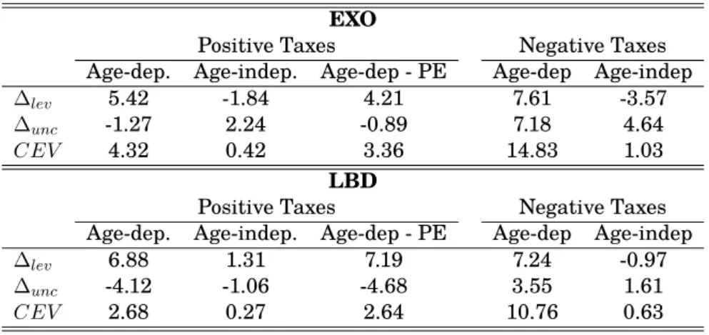
To substantiate this impression we consider an assessment of the origins of welfare gains
made possible by following the welfare decomposition proposed byHeathcote et al.[2008]. The
idea here is that welfare gains may be attained by a tax system that induces a better use of resources and/or better risk sharing. First, note that changes in the dispersion of wages are associated with both better opportunities to exploit the moments where wages are higher and the usual costs associated with the concavity of the utility function. Second, by making effort more productive a larger stock of capital permits more consumption for any given level of labor
supply. Both types of ’efficiency’ gains are captured by a level effect variable,∆lev, while risk
sharing is captured by an uncertainty effect variable,∆unc.
Let C0,t and L0,t denote, respectively, average consumption and average aggregate hours
worked bytyears old agents at the benchmark. LetC1,t andL1,t be the equivalent variables
at the alternative tax system. We then define∆lev through
X
t
βt−1
t Y
j=1
ψt
((1 + ∆lev)C0,t)1−ρt(1−L0,t)ρt 1−γ
=X
t
βt−1
t Y
j=1
ψt
C11,t−ρt(1−L1,t)ρt 1−γ
Table 8: Inequality: LBD. The table displays the evolution of inequality, measured by the variance of before
taxes, after taxes income and assets by age.
Variance by Age: Benchmark
20 30 40 50 60 Before Taxes Labor Income 0.0276 0.0870 0.1468 0.1999 0.2258 After Taxes Labor Income 0.0194 0.0564 0.0898 0.1184 0.1369 Assets 0.0591 1.4251 5.0995 9.2453 11.6269
Variance by Age: Optimum
20 30 40 50 60 Before Taxes Labor Income 0.0387 0.1200 0.1970 0.2498 0.2864 After Taxes Labor Income 0.0385 0.0998 0.1369 0.1434 0.1350 Assets 0.1123 2.7677 9.3800 15.2655 16.5205
Variance by Age: Benchmark (negative taxes)
20 30 40 50 60 Before Taxes Labor Income 0.0278 0.0883 0.1477 0.2017 0.2328 After Taxes Labor Income 0.0195 0.0567 0.0903 0.1196 0.1384 Assets 0.0548 1.4099 5.0805 9.2191 11.6235
Variance by Age: Optimum (negative taxes)
20 30 40 50 60 Before Taxes Labor Income 0.0340 0.1125 0.1865 0.2242 0.2253 After Taxes Labor Income 0.0187 0.0536 0.0847 0.1106 0.1266 Assets 0.1914 3.4935 9.3353 12.7612 10.1005
Next, lettingEdenote the unconditional expectation operator,21definep0through
X
t
βt−1
t Y
j=1
ψt
((1−p0)C0,t)1−ρt(1−L0,t)ρt 1−γ
=E
X
t
βt−1
t Y
j=1
ψt
c1t,−0ρt(1−lt,0)ρt
1−γ
where(ct,0, lt,0)tare benchmark allocations, andp1through
X
t
βt−1
t Y
j=1
ψt
((1−p1)C1,t)1−ρt(1−L1,t)ρt 1−γ
=E
X
t
βt−1
t Y
j=1
ψt
c1t,−1ρt(1−lt,1)ρt
1−γ
where(ct,1, lt,1)tare equilibrium allocations under the alternative policy.
We then define
∆unc≡ 1−p1
1−p0 −
1.
Before we describe our findings a final word about this decomposition is due. Ideally, we
would like to capture all ’smoothing’ effects, both inter-temporal and across states in our∆unc
measure by averaging consumption and labor supply on ages as well. A problem with this mea-sure in our context is that our preferences are age-dependent meaning that perfect smoothing across ages is never optimal.
We display welfare decomposition results in Table 10. For our main experiment, all the
gains from the tax reform are due to increased efficiency, as captured by the∆lev term. As
suggested by our discussion about inequality, risk sharing, broadly understood, worsens. In fact for the LBD specification, while the efficiency gains are equivalent to a 6.88% increase in average consumption, these are accompanied by a 4.12% loss due to increased volatility in
consumption. Table8displays the increase in the variance of after tax income induced by the
reform. For the exogenous model risk sharing contributes more than one percentage point