Some geometric models of
ancient astronomy with
Geogebra
Leandro Tortosa
University of Alicante, Alicante, Spain
[email protected]ABSTRACT. The main objective of this work is to review and simulate, with the help of GeoGebra, the most important geometric models used by the ancient astronomers to explain the mechanisms governing the trajectories of celestial bodies in the sky. It is well known that ancient astronomers like Ptolemy, Copernicus, Galileo, invented the same complex geometric systems of circles to explain the motion of the celestial bodies. It was not until Kepler, with the introduction of conics in the geometric models, that it was possible to accurately explain the observations with theoretical models.
1. An historic introduction
Plato (427-347 BCE), the Greek erudite, came to say that God, the creator of the universe, always using geometric procedures. In mathematics Plato's name is attached to the Platonic solids. In the Timaeus there is a mathematical construction of the elements (earth, fire, air, and water), in which the cube, tetrahedron, octahedron, and icosahedrons are given as the shapes of the atoms of earth, fire, air, and water. The fifth Platonic solid, the dodecahedron, is Plato's model for the whole universe. Plato's beliefs as regards the universe were that the stars, planets, Sun and Moon move round the Earth in crystalline spheres. The sphere of the Moon was closest to the Earth, then the sphere of the Sun, then Mercury, Venus, Mars, Jupiter, and Saturn and furthest away was the sphere of the stars.
For Aristotle (384-322 BCE), a little more realistic, the objects of mathematics are the forms drawn from nature, is the modification of the empirical regularities that occur in reality.
Since then, following the appearance of Euclid's Elements, points, lines, angles, circles and spheres ... the perfect forms, the regular polyhedra are going to become the only tools at our disposal to interpret nature. The imperfect forms are excluded and expelled from the mathematical universe.
can explain all natural phenomena. The understanding and mastery of nature to the scope of the human mind.
Aristotle placed Earth at the center of the universe and the moon's orbit is the line between order and chaos. Above the moon, the celestial world is perfect and everlasting, the kingdom of order. Below, the terrestrial world made up of four elements: earth, water, air and fire. An imperfect and unpredictable world; the kingdom of chaos.
However, an observable phenomenon breaks the perfect harmony of the celestial world. Erratic orbits of planets against the background of fixed stars. Hence its name, erratic. Sometimes there is even a step backwards in their orbits. How do these facts fit with a perfect and ideal geometric model?
Aristotle uses a model of spheres of ether in which the planets move, to be accelerating or braking. This model will remain untouched for two thousand years, astronomers still have to perform real mathematical prowess to fit the observations of the motion of the stars with the Aristotelian theory. To further explore in the history of ancient astronomy, we can see, among the extensive literature, [Aab01, Bru09].
2. The Ptolemy’s model
Claudius Ptolemy, an Alexandrian Greek astronomer who lived in the second century AD, devised a very sophisticated geometrical model in which only using circles it was possible to explain the movement of the astronomical objects.
The most important of Ptolemy's work that has survived is the Almagest, a treatise in 13 books. It gives in detail the mathematical theory of the motions of the Sun, Moon, and planets. In this work, he proposes an ingenious geometric model: the epicycles and deferent. Each planet, including the Sun and Moon, are assigned an imaginary circle called the deferent. The Earth is inside that circle, though not necessarily in the center. The planet rotates in a circle called the epicycle whose new center will be a point of the deferent circle. By moving the center of the epicycle along the deferent, the planet is moving toward or away from Earth, explaining the changes in brightness of the same planet observed at different times of the year.
In fact, Ptolemy did not believe that the planets moved in this way; however, this model fairly accurately explained everything that any astronomer could see in the sky. This model was taken as dogma and complicated mathematical calculations were performed to predict the position of the planets in the sky.
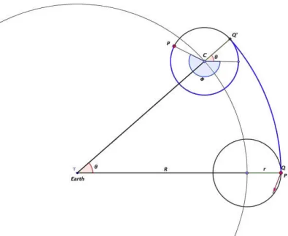
Figure 1: The planet P moving around the earth.
We obtain the following equation when the planet P describes a circle (epicycle) whose center is in a circle (deferent) whose center is the earth.
The coordinates of P relative to the center C are: (r cos
, r sin
). The coordinates of C relative to the origin (T) are: (R cos θ, R sin θ . Then, the coordinates of P relative to the origin of the deferent are:
sin
sin
cos
cos
r
R
y
r
R
x
. (1)
If we observe Fig. 1 we realize that the angles θ and
are not independent. The relationship between them is that the length of the arcs QQ’ and Q’P must be equal, that is,l QQ’ = l Q’P.
From the Fig. 1, we can establish that l QQ’ = R+r θ and, similarly,
l QQ’ =r θ+
). Therefore,R+r θ = r θ+
).Simplifying this expression, we conclude that
R
r
.Substituting in the expression (1) we obtain the equations of the planet P around the earth; they are
x
R
cos
r
cos
R
r
y
R
sin
r
sin
R
r
. (2)
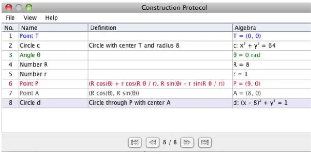
First, we start by defining the origin (T) and a circle of radius 8 units that will be the deferent. We then construct an angle θ fro to π usi g a slider. I our e a ple, e take R = 8 and r = 1. Later, we construct the point from the equations given by (2). At this point, we set the motion of the center of the epicycle around the deferent. Finally, we draw the epicycle with a circumference centered at A (a point on the deferent) and of radius r.
Fig. 2 shows an image of the previous construction.
Figure 2: Path of the planet P around the earth.
rates as it moves relative to the center of the deferent C around the earth, we will visualize the movements of advance and retreat.
Then, for example, if
2
l
(
')
l
(
Q
'
P
)
We obtain the following relation
2
R
r
r
.Thus, the equations of the planet in its epicycle will be given by
x
R
cos
r
cos
2
R
r
r
y
R
sin
r
sin
2
R
r
r
(3).
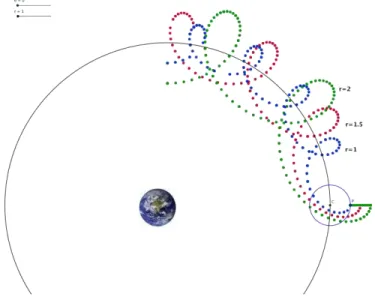
In Fig. 3 we have introduced the appropriate modifications in the construction with GeoGebra with the objective that the planet follows a trajectory given by the equations (3). Besides, a slider (r) has been introduced, so we can verify the different trajectories by varying the radius of the epicycle.
Figure 3: The planet P moves around the earth following the equations (3).
3. The Heliocentric theory
axis (see [Dre53]). According to Archimedes, Aristarchus of Samos (310–230 BCE) wrote of heliocentric hypotheses in a book that does not survive. Plutarch wrote that Aristarchus was accused of impiety for "putting the Earth in motion" (see, for example, [TM04]).
In a manuscript of De revolutionibus, Copernicus wrote, "It is likely that ... Philolaus perceived the mobility of the earth, which also some say was the opinion of Aristarchus of Samos", but later struck out the passage and omitted it from the published book [Dre53].
Copernicus' major theory was published in De revolutionibus orbium coelestium (On the Revolutions of the Celestial Spheres), in the year of his death, 1543, though he had formulated the theory several decades earlier. Copernicus' "Commentariolus" summarized his heliocentric theory. It listed the "assumptions" upon which the theory was based as follows [Ros04]:
1. There is no one center of all the celestial circles or spheres.
2. The center of the earth is not the center of the universe, but only of gravity and of the lunar sphere.
3. All the spheres revolve about the sun as their mid-point, and therefore the sun is the center of the universe.
4. The ratio of the earth's distance from the sun to the height of the firmament (outermost celestial sphere containing the stars) is so much smaller than the ratio of the earth's radius to its distance from the sun that the distance from the earth to the sun is imperceptible in comparison with the height of the firmament.
5. Whatever motion appears in the firmament arises not from any motion of the firmament, but from the earth's motion. The earth together with its circumjacent elements performs a complete rotation on its fixed poles in a daily motion, while the firmament and highest heaven abide unchanged.
6. What appear to us as motions of the sun arise not from its motion but from the motion of the earth and our sphere, with which we revolve about the sun like any other planet. The earth has, then, more than one motion.
7. The apparent retrograde and direct motion of the planets arises not from their motion but from the earth's. The motion of the earth alone, therefore, suffices to explain so many apparent inequalities in the heavens.
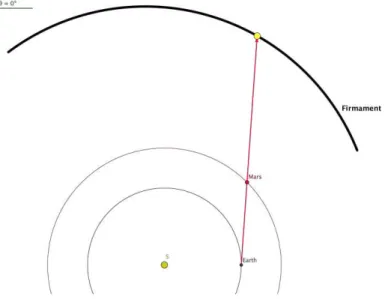
Figure 4: Retrograde motion of mars seen from the earth.
We have a slider in Fig. 4 (angle θ), which controls the whole animation. It is clearly observed, (following the trajectory of the yellow point in the arc simulating the firmament), that the retrograde motion of mars in the celestial sphere is due to the orbital motion of the earth around the sun.
4. The Kepler’s model
Undoubtedly, the name of Kepler in astronomy is linked to that of Tycho Brahe, as will be discussed briefly. These two colorful characters made crucial contributions to our understanding of the universe: T ho’s o ser ations were accurate enough for Kepler to discover that the planets moved in elliptic orbits, and his other laws, which gave Newton the clues he needed to establish universal inverse-square gravitation.
Tycho Brahe (1546-1601), was fascinated by astronomy, but disappointed with the accuracy of tables of planetary motion at the time. He decided to dedicate his life and considerable resources to recording planetary positions ten times more accurately than the best previous work. He achieved his goal of measuring to one minute of arc. This was a tremendous feat before the invention of the telescope. His aim was to confirm his own picture of the universe, which was that the earth was at rest, the sun went around the earth and the planets all went around the sun - an intermediate picture between Ptolemy and Copernicus.
remembered that there were just five perfect Platonic solids, and this gave a reason for there being six planets - the orbit spheres were maybe just such that between two successive ones a perfect solid would just fit. He convinced himself that, given the uncertainties of observation at the time, this picture might be the right one. However, that was before T ho’s results ere used. Kepler realized that T ho’s ork ould settle the question one way or the other, so he went to work with Tycho in 1600. Tycho died the next year, Kepler obtained the data, and worked with it for nine years.
He reluctantly concluded that his geometric scheme was wrong. In its place, he found his three laws of planetary motion:
I. The planets move in elliptical orbits with the sun at a focus.
II. In their orbits around the sun, the planets sweep out equal areas in equal times. III. The squares of the times to complete one orbit are proportional to the cubes of the average distances from the sun.
These are the laws that Newton was able to use to establish universal gravitation. Kepler was the first to state clearly that the way to understand the motion of the planets was in terms of some kind of force from the sun. However, in contrast to Galileo, Kepler thought that a continuous force was necessary to maintain motion, so he visualized the force from the sun like a rotating spoke pushing the planet around its orbit.
The three types of conic sections (i.e., parabola, ellipse and hyperbola) can be treated in a more unified form using a focus and directrix in polar coordinates. The analysis presented here assumes the focus is at the origin. Let F be a fixed point called the focus and
D be a fixed line called the directrix in a plane. Let e be the eccentricity and all points P of a conic section satisfy the equation:
e
PF
PD
.Basically, the eccentricity is given by the ratio of the distance from F to the distance from L. The conic section is:
(1) an ellipse when e < 1, (2) a parabola when e = 1, and (3) a hyperbola when e > 1.
The conic section in polar coordinates has the following form:
r
ep
1
e
cos
,where e is the eccentricity and p is the distance to the directrix.
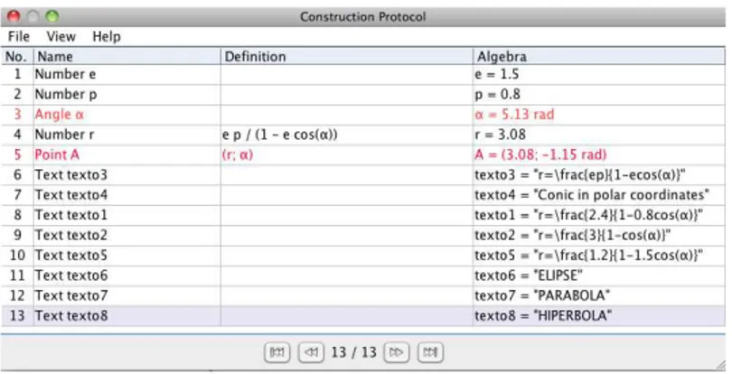
As we can see, the protocol is very simple and has the following steps: 1. We construct the slider e (the eccentricity).
2. We construct a slider p (to vary the distance to the directrix). 3. We construct the slider (angle).
4. We define the equation of the conic section in polar coordinates for a concrete value of the parameters e, p,.
5. We define the point A in polar coordinates as A(r; ). 6. The following steps are text chains in the image.
Remark that when we move the slider, then the point A will describe the trajectory of the conic section defined by the parameters e and p. We have an example in the following figure:
Figure 5: Conic sections in polar coordinates.
eccentricity e between 0 and 1, we see different forms of the ellipse in terms of its eccentricity. The same is true for the hyperbola when the eccentricity is greater than 1.
Thanks to the simplicity of the equation of the conics in polar coordinates and taking account of Kepler's laws, it would not be too difficult (with the help of GeoGebra), to draw the orbits of the planets in the solar system, both inner and outer planets. We must take into account planetary data, particularly those associated with distance from the sun and
the e e tri it of ea h or it. For e a ple, ars’ or it a e des ri ed the polar
equation
r
1.52
1
0.09cos
,which may be easily represented in a dynamic geometry system like GeoGebra, as we have seen before.
Bibliography
[Aab01] A. Aaboe–Episodes from the early history of astronomy, Oxford University Press, 2001.
[Bru09] G. van Brummelen–The mathematics of the Heavens and the Earth: the early history of trigonometry, Princeton University Press, 2009.
[Dre53] J.L.E. Dreyer–A history of astronomy from Thales to Kepler, Dover, New York, 1953. [Eva98] J. Evans–The history practice of ancient astronomy , Oxford University Press, 1998. [Ros04] E. Rosen–Three Copernican treatises: the Commentariolus of Copernicus; the letter
against Werner; the narratio prima of Rheticus, Dover, New York, 2004.