www.biogeosciences.net/5/1669/2008/
© Author(s) 2008. This work is distributed under the Creative Commons Attribution 3.0 License.
Biogeosciences
Temporal variability of the anthropogenic CO
2
storage in the
Irminger Sea
F. F. P´erez1, M. V´azquez-Rodr´ıguez1, E. Louarn2,3, X. A. Pad´ın1, H. Mercier4, and A. F. R´ıos1 1Instituto de Investigaciones Marinas, CSIC, Eduardo Cabello 6, 36208 Vigo, Spain
2Laboratoire de Chimie Marine, Institut Universitaire Europ´een de la Mer, Plouzan´e, France 3Station Biologique de Roscoff, CNRS UPMC, B.P. 74, 29682 Roscoff, France
4Laboratoire de Physique des Oc´eans, CNRS Ifremer IRD UBO, IFREMER Centre de Brest, B.P. 70, 29280 Plouzan´e, France Received: 29 February 2008 – Published in Biogeosciences Discuss.: 11 April 2008
Revised: 14 November 2008 – Accepted: 14 November 2008 – Published: 11 December 2008
Abstract. The anthropogenic CO2 (Cant) estimates from cruises spanning more than two decades (1981–2006) in the Irminger Sea area of the North Atlantic Sub-polar Gyre reveal a large variability in the Cant stor-age rates. During the early 1990’s, the Cant storage rates (2.3±0.6 mol C m−2yr−1) doubled the average rate for 1981–2006 (1.1±0.1 mol C m−2yr−1), whilst a remark-able drop to almost half that average followed from 1997 onwards. The Cant storage evolution runs parallel to chlorofluorocarbon-12 inventories and is in good agreement with Cant uptake rates of increase calculated from sea sur-facepCO2measurements. The contribution of the Labrador Seawater to the total inventory of Cantin the Irminger basin dropped from 66% in the early 1990s to 49% in the early 2000s. The North Atlantic Oscillation shift from a positive to a negative phase in 1996 led to a reduction of air-sea heat loss in the Labrador Sea. The consequent convection weakening accompanied by an increase in stratification has lowered the efficiency of the northern North Atlantic CO2sink.
1 Introduction
The ocean is a CO2 sink that during the 1990s has re-moved 2.2±0.4 Pg C yr−1from the atmosphere out of the to-tal 8.0±0.5 Pg yr−1of anthropogenic carbon (Cant)emitted to the atmosphere directly from human activities (Canadell et al., 2007). The North Atlantic Subpolar Gyre (NASPG) has the largest Cantinventory per unit area (∼80 mol C m−2
Correspondence to:F. F. P´erez ([email protected])
Fig. 1. (a)Map showing the Irminger Sea ends of the North Atlantic cruises used to assess the temporal evolution of the Cant storage. The acronyms stand for: R = Reykjanes Ridge, BFZ = Bight Fracture Zone and CGFZ = Charlie Gibbs Fracture Zone.(b)Main water masses (cLSW = classical Labrador Seawater; uLSW = upper Labrador Seawater; NEADW = North East Atlantic Deep Water; DSOW = Denmark Strait Overflow Water) present in the Irminger basin and analysed in terms of Cantinventory distributions over time. The density (σθ, in kg m−3)boundaries were established following Kieke et al. (2007) and Yashayaev et al. (2008).
MOC is closely related with the variability of Labrador Sea-water (LSW) formation rates (H´at´un et al., 2005; Latif et al., 2006; B¨oning et al., 2006). On the other hand, the long-term evolution of the MOC such as the possible weakening during the 21st century might be related to a decrease in the density of the Denmark Straight Overflow Water (DSOW) and the Iceland-Scotland Overflow Water (ISOW) (Cubasch et al., 2001; IPCC, 2007; B¨oning et al., 2006). These water masses meet in the Irminger Sea, where the Deep Western Boundary Current originates (Yashayaev et al., 2008, here-inafter Y’08).
The Irminger basin has been proposed as a LSW forma-tion region (Pickart et al., 2003; Falina et al., 2008), in ad-dition to the Labrador Sea. Independently of the formation region, two modes of LSW are typically defined: the clas-sical LSW (cLSW, sometimes referred to as deep LSW) and the less dense upper LSW (uLSW) (Pickart et al., 1997). The LSW is formed in winter, when deep convection caused by intense air-sea heat loss results in the formation of homo-geneous layers that can exceptionally reach depths of up to 2000 m (Kieke et al., 2006, hereinafter K’06). The ambient stratification and wind forcing intensity are determinant fac-tors in this convective process (Dickson et al., 1996; Curry et al., 1998; Lazier et al., 2002). The convection activity in the Labrador Sea is related to the persistence and phase of the North Atlantic Oscillation (NAO) index. A positive NAO phase causes the intensification of winds and heat loss (sur-face cooling) in the Labrador Sea, fostering convection pro-cesses. During the early 1990’s, the strongly positive NAO index forced an impressive and exceptional convection activ-ity down to more than 2000 m (Dickson et al., 1996; Lazier et al., 2002; H¨akkinen et al., 2004; Y’08). This resulted in the formation of the thickest layer of cLSW observed in
the past 60 years (Curry et al., 1998). This energetic con-vection period abruptly ended in 1996 with the shift of the NAO index to a negative phase. Nonetheless, weaker con-vection events (to less than 1000 m depth on average) contin-ued to take place in the central Labrador Sea and formed the less dense uLSW. This water mass was first detected and de-scribed by Pickart et al. (1997) in the western Labrador Sea. Alternatively, the uLSW was spotted successively during the second half of the 1990’s (Azetsu-Scott et al., 2003, here-inafter AS’03; Stramma et al., 2004). Decadal time series of layer thicknesses of both LSW types corroborate that, far from exceptional, uLSW is an important product of the con-vection activity in the Labrador Sea (K’06). These time se-ries show that the strong formation processes of cLSW in the early 1990’s are actually the exceptional events. The obser-vations point to a slight chlorofluorocarbon-12 (CFC12) con-centration decline (within the analytical uncertainty range, though) towards the end of the decade in the cLSW body (AS’03), following a strong CFC12 concentration increase that occurred in the early 1990s. This CFC12 decrease was also observed during the early 2000’s in the Labrador and Irminger Seas (Kieke et al., 2007, hereinafter K’07). The fluctuations of convection in the NASPG can modify the ex-pected oceanic Cant uptake rates in a likewise and parallel manner to CFCs.
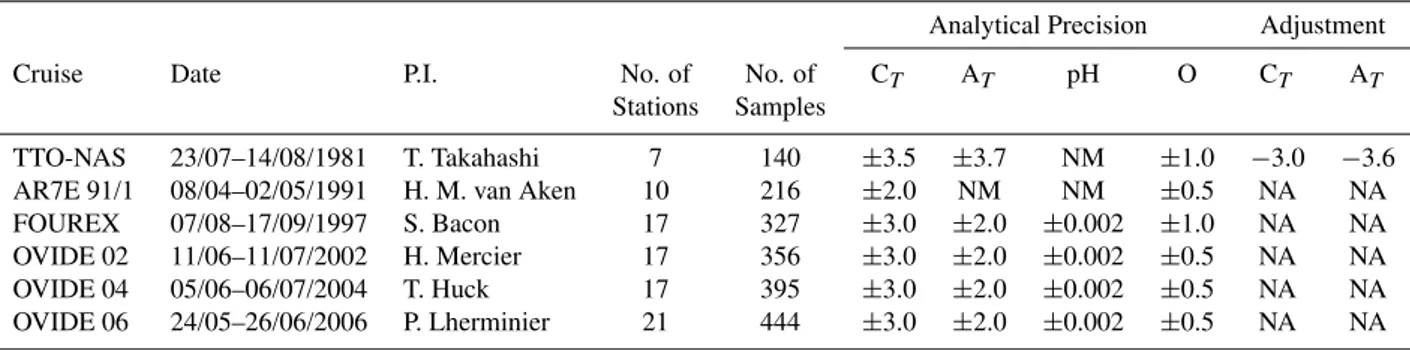
Table 1.Summary of cruises showing the analytical precision of the measurements for the main variables used in Cantestimation.Nstands for the number of NM means “Not Measured” andN Astands for “No Adjustment made”. In any case, units for CT, AT and oxygen (O) are inµmol kg−1.
Analytical Precision Adjustment
Cruise Date P.I. No. of No. of CT AT pH O CT AT Stations Samples
TTO-NAS 23/07–14/08/1981 T. Takahashi 7 140 ±3.5 ±3.7 NM ±1.0 −3.0 −3.6 AR7E 91/1 08/04–02/05/1991 H. M. van Aken 10 216 ±2.0 NM NM ±0.5 NA NA FOUREX 07/08–17/09/1997 S. Bacon 17 327 ±3.0 ±2.0 ±0.002 ±1.0 NA NA OVIDE 02 11/06–11/07/2002 H. Mercier 17 356 ±3.0 ±2.0 ±0.002 ±0.5 NA NA OVIDE 04 05/06–06/07/2004 T. Huck 17 395 ±3.0 ±2.0 ±0.002 ±0.5 NA NA OVIDE 06 24/05–26/06/2006 P. Lherminier 21 444 ±3.0 ±2.0 ±0.002 ±0.5 NA NA
2 Dataset and method
Six cruises spanning through 25 years (1981–2006) of high-quality carbon measurements in the Irminger Sea area have been selected for this study. These are the TTO-NAS leg 41, AR7E 91/12, FOUREX/WOCE A253and the OVIDE 2002, 2004 and 2006 cruises (Fig. 1a, Table 1). The bottle and CTD data yielded very similar property profiles. Since bot-tle data includes all carbon-related analysis, only botbot-tle data was used in this study. Unlike in the most recent cruises of FOUREX or throughout the OVIDE project, the TTO-NAS and AR7E 91/1 analytics did not include certified ref-erence materials for their total inorganic carbon (CT) mea-surements. For the TTO-NAS, Tanhua et al. (2005) per-formed a cross-over analysis with an overlapping more recent cruise. Based on a comparison with modern Certified Refer-ence Material-referRefer-enced data, they suggest a correction for TTO-NAS CT measurements of−3.0µmol kg−1, which has been applied to our dataset. In order to evaluate and interpret the variations of Cant rates of storage we have focused on six water masses delimited by the density (σθ)intervals es-tablished following K’07 and Y’08, namely: from the upper 100 m toσθ=27.68 kg m−3we find the sub-surface layer; The uLSW is found between 27.68<σθ<27.76 kg m−3; cLSW between 27.76<σθ<27.81 kg m−3; North East Atlantic Deep Water (NEADW, which includes the ISOW contributions) is delimited by 27.81<σθ<27.88 kg m−3, and DSOW by
σθ>27.88 kg m−3(Fig. 1b).
To estimate the anthropogenic CO2theϕC◦T method from V´azquez-Rodr´ıguez et al. (2008a) is applied (refer to Ap-pendix A for details). It is a data-based, back-calculation method that constitutes an alternative version of the classi-cal1C* approach (Gruber et al., 1996). TheϕC◦T method is not CFC-reliant and uses sub-surface layer (100–200 m)
1http://cdiac3.ornl.gov/waves/
2http://whpo.ucsd.edu/data/repeat/atlantic/ar07e/ar07ea/
ar07e a hy1.csv
3http://whpo.ucsd.edu/data/onetime/atlantic/a25/index.htm
data from the whole Atlantic as the only reference to build the parameterizations needed. This sub-surface layer avoids the seasonal variability of surface properties, thus making the derived parameterizations more representative of water mass formation conditions. The method also takes into account the temporal variation of the CO2air-sea disequilibrium (1Cdis). The overall uncertainty of the method has been estimated in 5.2µmol kg−1 by means of random error propagation over the precision limits of the parameters involved in the calcula-tion of Cant(refer to Appendix A). Regarding the specific in-ventory estimates, errors were estimated using a perturbation procedure for each layer and the total water column. They were calculated by means of random propagation with depth of a 5.2µmol kg−1standard error of the Cant estimate over 100 perturbation iterations, and are given in Table 2. As-suming that the uncertainties attached to the Cantestimation method are purely random and do not introduce biases, the final error included in Fig. 4 is calculated by propagating the individual errors associated to the samples. They reflect both measurement and parameterization errors.
3 Results
Table 2.Temporal evolution (1981–2006) of the average values of thickness (±STD), salinity, potential temperature, AOU, Cant, percentage of Csatantand percentage contribution to the specific inventory of Cantin the five considered water masses. The averages come from bottle data and the uncertainties stand for the error of the mean. Total specific inventories are given by the red line in Fig. 4.
Year Thickness Salinity θ AOU Cant %Csatant %Inventory (m) (◦C) (µmol kg−1) (µmol kg−1)
Sub-surface layer
1981 419±410 34.902±0.001 5.118±0.005 20.4±0.3 29.3±1.5 95±5 22.6±1.1 1991 144±141 34.981±0.002 5.229±0.007 19.0±0.4 34.6±1.8 92±5 8.0±0.4 1997 414±406 34.893±0.001 5.134±0.003 21.0±0.1 38.8±0.8 92±2 20.7±0.4 2002 405±397 34.949±0.001 5.362±0.003 24.6±0.2 42.1±0.8 90±2 22.3±0.4 2004 556±544 34.967±0.001 5.611±0.002 23.8±0.1 43.5±0.6 89±1 30.3±0.4 2006 552±540 34.973±0.001 5.587±0.002 23.7±0.1 43.4±0.6 86±1 29.6±0.4
uLSW
1981 829±811 34.865±0.001 3.539±0.004 28.1±0.2 25.2±1.2 84±5 38.4±1.8 1991 713±698 34.889±0.001 3.577±0.004 24.2±0.2 31.3±0.9 86±3 35.8±1.0 1997 506±496 34.869±0.001 3.520±0.003 35.9±0.1 32.1±0.7 79±2 21.0±0.4 2002 686±671 34.896±0.001 3.803±0.003 35.0±0.1 33.7±0.6 75±2 30.2±0.5 2004 673±659 34.888±0.001 3.710±0.003 37.2±0.1 33.2±0.7 71±2 27.9±0.6 2006 646±633 34.901±0.001 3.822±0.002 34.1±0.1 34.4±0.6 70±2 27.5±0.4
cLSW
1981 557±546 34.918±0.002 3.375±0.006 39.2±0.4 18.6±1.7 62±9 19.1±1.8 1991 970±948 34.878±0.001 3.137±0.004 32.5±0.2 24.6±0.9 68±3 38.1±1.3 1997 983±960 34.868±0.001 2.989±0.003 30.8±0.1 29.9±0.7 74±2 37.8±0.9 2002 678±663 34.897±0.001 3.185±0.003 38.8±0.2 27.2±0.7 61±3 24.1±0.6 2004 546±534 34.902±0.001 3.232±0.004 40.5±0.2 26.8±0.9 58±3 18.3±0.6 2006 529±518 34.920±0.001 3.355±0.003 40.6±0.2 27.1±0.8 56±3 17.8±0.5
NEADW
1981 686±672 34.948±0.001 2.980±0.004 44.3±0.3 14.1±1.2 47±9 17.7±1.6 1991 746±730 34.940±0.001 2.925±0.003 48.4±0.1 12.9±0.8 36±6 15.4±0.9 1997 754±738 34.924±0.001 2.813±0.004 44.2±0.2 18.5±1.0 46±5 18.0±0.9 2002 762±745 34.917±0.001 2.759±0.002 43.7±0.1 20.7±0.7 47±3 20.6±0.7 2004 755±739 34.916±0.001 2.753±0.003 44.4±0.2 21.7±0.8 47±4 20.5±0.8 2006 787±770 34.929±0.001 2.850±0.003 43.2±0.1 22.1±0.8 46±3 21.5±0.7
DSOW
1981 98±96 34.892±0.002 1.680±0.010 36.6±0.4 12.7±2.5 43±20 2.3±0.4 1991 134±131 34.897±0.001 1.778±0.005 41.6±0.2 12.7±1.2 36±9 2.7±0.3 1997 94±93 34.894±0.002 1.720±0.008 38.8±0.4 19.8±2.2 50±11 2.4±0.3 2002 110±108 34.887±0.001 1.721±0.004 39.4±0.2 18.7±1.3 43±7 2.7±0.2 2004 112±110 34.869±0.001 1.534±0.004 36.3±0.2 21.1±1.1 47±5 3.0±0.2 2006 132±129 34.906±0.001 1.866±0.005 37.6±0.2 21.6±1.0 46±4 3.5±0.2
LSW formation at the Irminger Sea (Pickart et al., 2003), which caused the saltier NEADW signal to shrivel. The same year, the LSW layer also thickened substantially in the Labrador Sea (Fig. 12 in K’06). Since the AR7E cruise was carried out shortly after the winter season, the sub-surface layer thickness is seen to decrease substantially (Table 2). In 1997, the low salinity LSW invaded lower layers, beyond the 2000 m depth, while surface stratification slightly increased. The temperature of the cLSW reaches its minimum values for the period of observation, in agreement with Y’08, who ob-served that this minimum had been developing since at least
one year earlier. The DSOW temperature signature (θ <2◦C)
0
1000
2000
3000
0
1000
2000
3000
0
1000
2000
3000
0
1000
2000
3000
38ºW
40ºW 36ºW 34ºW 32ºW 30ºW 40ºW38ºW36ºW 34ºW 32ºW 30ºW42ºW 40ºW 38ºW 36ºW 34ºW 40ºW 35ºW 30ºW 40ºW 35ºW 30ºW 40ºW 35ºW 30ºW
8 7 6 5 4 3 2 1 35.2
35.1
35.0
34.9
34.8 60 50 40 30 20
10 0 60 50 40 30 20
10 0
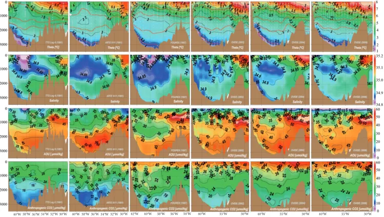
Fig. 2. Vertical profiles from bottle data of, potential temperature (Thetaθ, in◦C), Salinity, AOU (µmol kg−1)and Cant(µmol kg−1)for the six cruises shown in Fig. 1a. Depth is indicated in the left-hand axis in dbar. The colour scale in each of the variables is the same for all years to facilitate comparison. It must be noticed that the eastern and western ends of the different sections are not necessarily identical. The red lines in theθplots represent the same isopycnals shown in Fig. 1b, separating the main water masses in the Irminger basin. The thick light-grey dots in theθplots represent the stations and bottle sampling spots. The data here plotted is the same used to compute Cantstorages and other results presented in this work.
Rhein et al., 2007; Y’08). The described thermohaline evo-lution concurs with theθ/S results shown by Y’08 for the LSW core: A salinity and temperature minimum is recorded in 1996 at the Irminger Sea (which is two years behind the
θ/Sminimum at the Labrador Sea). It is followed by a pro-gressive salinization and warming due to lateral mixing that can be observed along theσ1=36.93 isopycnal and extends to the rest of LSW density range (Sarafanov et al., 2007; Y’08). In 1981, there is a manifest stratification between the nearly oxygen-saturated sub-surface waters and the older NEADW that is clearly identified from the AOU profiles. The relative AOU minimum at the bottom of the western part in the Irminger Basin indicates the marked presence of DSOW. The Cant concentrations follow a similar pattern to AOU: high values, close to saturation (32µmol kg−1), near the surface and lower values (∼45% of saturation) towards the bottom. During the first deep convection events in the Irminger Sea in the early 1990’s there was a significant and parallel increase in the Cant and oxygen loads in the upper 1500 m. Nevertheless, the NEADW region shows higher AOU along with slightly lower (around 15%) Cant values than in 1981, denoting that ventilation does not reach as deep
a)
b)
d)
c)
1)
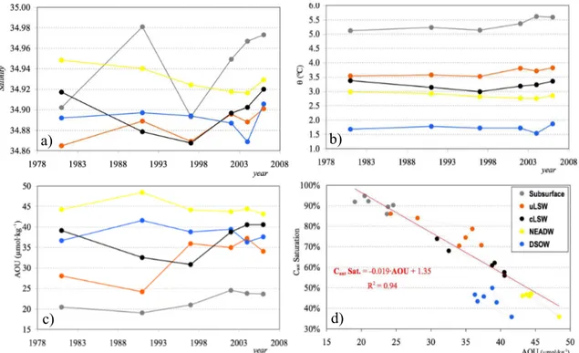
Fig. 3. Data from Table 2 plotted to show the temporal evolution (1981–2006) of the average(a)Salinity, (b) θ (◦C) and(c) AOU (µmol kg−1)of the main water masses in the Irminger basin. (d)shows the correlation found between AOU and the % saturation con-centration of Cant.
rising in response to the atmospheric CO2 increase. Con-versely, weaker winds and buoyancy forcing associated with the low NAO index period during OVIDE provoked an in-crease in the stratification of the upper layers. This precluded local ventilation and translated into a dilution of Cantin the cLSW layer due to the permanently active isopycnal mixing. The Cantin the NEADW increases continuously suggesting incorporation of young water by entrainment downhill of the Iceland-Scotland sills. Finally, the DSOW flow (Olsson et al., 2005; Tanhua et al., 2008) appears more ventilated with respect to previous years and it also displays small Cant rela-tive maxima. The observed increase of Cantin the NEADW and DSOW can derive from vigorous mixing processes, but it might also reflect the increase of the Cant content in the Arctic source waters.
The average values (from bottle data) and associated un-certainties in salinity, temperature, AOU, Cantand saturation concentration of Cant(Csatant)for each cruise and layer (Fig. 1) are summarised on Table 2 and Fig. 3. The average thickness of the layers and their percentage contribution to Cant spe-cific inventories are also given in Table 2. The thickness was calculated as the average distance between layers weighed by the separation between stations. The averages for the rest of properties were computed integrating vertically and hor-izontally, and then dividing by the area of the correspond-ing layer. The Csatant is estimated from the average tempera-ture and salinity of the layer, assuming full equilibrium of
former would represent the highly ventilated young waters from the winter mixed layer (WML) whereas the latter would stand for the older components. The deviations from this hy-pothetical mixing line can be due to lateral advection, to in-terannual or decadal variability of water mass formation or to differential biological activity rates.
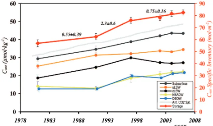
The temporal evolution of the average Cantin each of the five layers is plotted in Fig. 4. The Cantestimation approach used is theϕC◦T method (Appendix A). The sub-surface layer (Fig. 1b) increases its Cant steadily and sustains its high %Csatant (>86%) while trying to catch up with the rising at-mospheric CO2concentrations. The uLSW trend from 1981 to 1991 follows its upper bound sub-surface layer, keeping up with the atmospheric CO2 increase and maintaining its %Csatant. The maximum thinning of the uLSW layer from 1981 to 1997 (Table 2) coincides with the end of the max-imum convection period in the Irminger Sea (K’06). The cLSW almost doubled its thickness and average Cant con-tent during this period of time (Table 2 and Fig. 3d) at a rate even superior to the atmospheric one. All of it derives from the increased convection processes that occurred in the NASPG between 1991 and 1997 (K’06). The noteworthy de-crease in Cantand layer thickness during the OVIDE cruises caused by the hindered ventilation entails the increase in the AOU levels due to isopycnal mixing. In the NEADW layer, Cantshows a large increment from 1991 to 1997 parallel to the salinity and AOU drop. This suggests the possibility of important diapycnal mixing with the upper re-ventilated cLSW. The DSOW layer will represent a very small contri-bution (2–3%, Table 2) to Cantstorage in the Irminger basin given its small thickness. It shows an analogous behaviour to NEADW, i.e., there is an increase in average Cant from 1991 to 1997, matched with a drop in AOU caused by the incorporation of young water by entrainment downhill of the Iceland-Scotland sills.
Regarding the temporal evolution of the Cantstorage rate, a global increase at different paces is observed. From 1981 to 2006 the average rate of increase in the specific Cant inven-tory for the Irminger Sea has been 1.1±0.1 mol C m−2yr−1. During the early 1990’s, this rate was more than twice the mean (2.3±0.6 mol C m−2yr−1). Compared with this period of exacerbated Cantstorage rate in the Irminger Sea, the av-erage storage rate during the following decade (1997–2006) underwent an important fall (Fig. 4) that was estimated in
−1.6±0.4 mol C m−2yr−1. The average Cantstorage rate of 0.75±0.16 mol C m−2yr−1during the FOUREX-OVIDE pe-riod was found to be significantly different from that of the early 1990’s (p-value<0.05). Based on the rapid water mass renewal in the Irminger compared to the Cantrate of increase in the ocean, it can be reasonably assumed that the Cant con-centrations in the different layers found in the studied section can be extrapolated to the whole Irminger basin. Therefore, the above data was extrapolated to cover the Irminger basin (0.58×10⁶km2, taking the FOUREX section and the Den-mark Strait as the southern and northern boundaries,
respec-Fig. 4. Temporal evolution (1981–2006) of the average Cant (µmol kg−1)stored in the subsurface layer (dark grey line), uLSW (orange line), cLSW (black line), NEADW (yellow line) and DSOW (blue line). The continuous grey line shows the 100% Cant saturation of water masses in equilibrium with the atmosphere over time, following the atmospheric CO2increase. The evolution of the specific inventory (in mol C m−2)of Cantin the Irminger basin is given by the thick red line, and its values can be read on the right-hand y-axis. The numbers above this line stand for the rates of increase of Cantstorage (in mol C m−2yr−1)for the time peri-ods (from left to right) of 1981–1991, 1991–1997 and 1997–2006, respectively.
tively) and give estimates of total inventories, admittedly of the uncertainties attached to this practice. They have been es-timated in 0.26±0.02 and 0.38±0.01 Gt C for the years 1981 and 2006, respectively.
4 Discussion
which decreases from 1997 to 2002 (Fig. 4). According to AS’03, the marked increase in CFC12 concentrations prior to 1995 in the uLSW core reduced to almost standstill from that point until 2000. This result is also in good agreement with the patterns of average Cantobtained for the same years and region in this study (Fig. 4). K’07 have pointed that this significant increase in CFC12 inventories in the uLSW for the NASPG best describes the situation in the Labrador Sea, rather than in the Irminger, where the CFC12 inventory has a more subtle increase during that period. In spite of this remark, our Cant results for the uLSW follow the expected trend, within the associated error margins. With respect to the NEADW and DSOW, AS’03 have shown that, from 1991 to 2000, the CFC12 concentration in the Labrador Sea in-creased up to 80% in both the NEADW and DSOW layers. Whilst this happened at a steady rate in the case of NEADW, the interannual variability was larger for DSOW. Over the same period, the Cant storages here obtained increased by 50% and 40% in the NEADW and DSOW layers, respec-tively. There are a few differences in the environmental be-havior of CFCs and CO2 that may account for the dissimi-larities in magnitude of their inventories. The former is not affected by the Revelle factor, it has a greater solubility in cold waters and its atmospheric rate of increase is different to that of CO2.
Although the NASPG has a net gain of Cant by horizon-tal advection (Mikaloff-Fletcher et al., 2006; ´Alvarez et al., 2003, hereafter A’03), estimating how much it is stored and how much of that comes from direct exchange with the at-mosphere entails certain difficulty. An indirect estimate of the air-sea Cant fluxes can be obtained by combining Cant storage results with horizontal transports into carbon budget balances from closed box studies (as in A’03 and Mikaloff-Fletcher et al., 2006). The Cantstorage rate for the Irminger Sea was first estimated by A’03 in 1.5±0.3 mol C m−2yr−1. For that calculation they assumed a fixed Cantrate of increase of 0.85µmol kg−1yr−1 and estimated also the mean pene-tration depth (MPD, as in Broecker et al., 1979) using data from the WOCE A20 and FOUREX cruises for the 1990– 1997 time period. Assuming a transient steady state (TSS, Keeling and Bolin, 1967) for Cant, the MPD is defined as the quotient between the specific inventory of Cant in the water column and the Cantconcentration in the mixed layer (Cmlant). The model results presented in Tanhua et al. (2006) demonstrate that the TSS assumption is indeed valid for Cant in this part of the North Atlantic Ocean. A high MPD nor-mally indicates that large amounts of Cant have penetrated in the water column following strong vertical convection processes (>1000 m depth) generated in the considered re-gion, and vice versa. A’03 calculated an average and con-stant MPD for the Irminger basin of 1739±381 m by ap-proximating Cmlant≈Csatantin the corresponding sampling years. The average Cant storage rate for the 1981–2006 period in the Irminger Sea here obtained is 1.1±0.1 mol C m−2yr−1. The calculated average MPD for the considered years is
1715±63 m. This is quite in agreement with A’03, although the MPD values are seen to vary, especially in the strong convection periods such as from 1991–1997. Also, Tan-hua et al. (2006) using an OGCM have shown that devi-ations from the TSS behaviour are possible in the SPNA due to the variability in deep water formation. Specifically, the MPD in the Irminger basin for the years 1981, 1991, 1997, 2002, 2004 and 2006 are, respectively: 1835±140, 1657±88, 1808±72, 1678±56, 1679±54 and 1632±42 m. The 1.5±0.3 mol C m−2yr−1 estimate from A’03 is larger than the average 1.1±0.1 mol C m−2yr−1here obtained and, anyhow, lower than the estimated rate, between 1991 and 1997, of 2.3±0.6 mol C m−2yr−1. Some factors account-ing for the temporal variability of Cantstorage rates may ex-plain some of these discrepancies, primarily: a) The time variability of the MPD can affect notoriously the Cant stor-age rates, especially between 1991 and 1997 (8% larger than the average). There can exist exceptional interannual stages where the storage rates can amount up to twice (1991–1997) or almost half (1997–2006) the long-term average; b) The Cant rate of increase must consider the dependence of the Csatant with temperature, which is intimately connected with the Revelle factor (it describes how the pCO2 in seawater changes for a given change in CT, and vice versa). The ca-pacity for ocean waters to take up Cant is inversely propor-tional to the Revelle factor, which depends on temperature. The Cantrates of storage can change∼2% per◦C.
Our observations in the Irminger Sea can also be com-pared with other works on the secular variation of sea sur-facepCO2that cover larger areas. In the NASPG, Lef`evre et al. (2004) reported a mean increase of 1.8µatm yr−1between 1982 and 1998. This corresponds to a1CT=0.77µmol kg−1 per annum for an average sea surface temperature of 5◦C in the Irminger Sea. If an average MPD of 1715 m is considered for this region and time period, the above 1pCO2 translates into a Cant storage rate that in-creases by 1.35 mol C m−2yr−1. This is very close to the 1.22±0.03 mol C m−2yr−1estimated here from Fig. 4 for the 1981–1997 period. From sea surface pCO2 measurements Schuster and Watson (2007) showed that the sink of atmo-spheric CO2in the whole North Atlantic was subject to im-portant interannual variability. They estimated an annual de-crease of the North Atlantic uptake of−1.1 mol C m−2yr−1 between 1997 and the mid-2000’s. They argued that the main causes for this change were the declining rates of win-tertime mixing and ventilation between surface and sub-surface waters due to increasing stratification. In the present work we have estimated this same rate of decrease to be
wintertime 1995. According to Schuster and Watson (2007), this corresponds to an annual decrease of the Cantstorage of
−1.6 mol C m−2yr−1, which is in excellent agreement with our estimates.
In summary, the general decline of the NASPG CO2sink is supported by the data here obtained and it is corroborated by other results like those from Schuster and Watson (2007) or Corbi`ere et al. (2007). There is a documented variability of the Labrador Sea deep convection that reached its maximum activity during the early to mid 1990s, correlated with posi-tive NAO phases. The maximum Cantstorage rate occurred during this maximum convection period. The observed con-vection decrease since 1997 in the NASPG is mainly tied to the enhanced stratification and the consequent reduced heat loss in the northern North Atlantic (Lazier et al., 2002; AS’03; K’07). All these fluctuations are embodied in the NAO index variability. The above factors have a direct influ-ence on the physical pump of CO2and add to the changes in the buffer capacity of surface waters to aggravate the capac-ity of the North Atlantic as a CO2sink.
Appendix A
The ϕC◦T method (V´azquez-Rodr´ıguez et al., 2008a) is a process-oriented biogeochemical approach to estimate Cant. It is an alternative to existing process-based Cantestimation methods such as the1C* (GSS’96) or TrOCA (Touratier et al., 2007). The distinctive characteristics of theϕC◦T method are:
1. The sub-surface layer (100–200 m) is taken as a ref-erence for characterising the properties of the water masses at their respective formation times. The variabil-ity of the conservative properties of greatest importance in Cantestimation (θ,S, NO, PO) is at least one order of magnitude smaller than in the surface layer. In addi-tion, the thermohaline variability of the surface layer en-closes and represents all water masses outcropped in the Atlantic Ocean. The use of data from the sub-surface layer reduces the sparseness of data available for pa-rameterizations given the high amount of data for sub-surface waters at any season compared to the scarce sur-face winter data.
2. The air-sea disequilibrium (1Cdis)is parameterized at the sub-surface layer first using a short-cut method to estimate Cant. Since the average age of the water masses in the 100–200 m depth domain, and most importantly in outcropping regions, is under 25 years, the use of the short-cut method to estimate Cantis appropriate (Matear et al., 2003).
3. TheA◦T and1Cdisparameterizations (in terms of con-servative tracers) obtained from sub-surface data are ap-plied directly to calculate Cant in the water column for
waters above the 5◦C isotherm and via an OMP
ap-proach (like in GSS’96) for waters withθ <5◦C. This
approach especially improves the estimates in cold deep waters that are subject to strong and complex mixing processes and represent an enormous volume of the global ocean (∼86%). One important aspect in this pro-cess is that, unlike for the1C* method, CFC data are not necessary to make Cant predictions, since none of theA◦T or1Cdisparameterizations are CFC-reliant. Following the work from Matsumoto and Gruber (2005), the ϕC◦T method proposes an approximation to the hori-zontal (spatial) and vertical (temporal) variability of1Cdis (11Cdis)in the Atlantic Ocean in terms of Cantand1Cdis itself. Also, the decrease of preindustrialA◦T due to CaCO3 dissolution changes projected from models (Heinze, 2004) and the effect of rising sea surface temperatures on the pa-rameterized A◦
T were corrected in our calculations. These two last corrections are minor and would be very diffi-cult to quantify directly through measurements. However, they should still be considered if a maximum 4µmol kg−1 bias (2µmol kg−1on average) in Cantestimates wants to be avoided. Following several in-detail evaluations of the un-certainties in Cant evaluation through back-calculation ap-proaches (Gruber et al., 1996; Gruber, 1998; Sabine et al., 1999; Wanninkhof et al., 2003; Lee et al., 2003), random errors were propagated over the precision limits of the vari-ous measurements required for solving their Cantestimation equations. TheA◦T parameterization here obtained has an as-sociated uncertainty two times lower than in GSS’96, while the uncertainties for1Cdisvary between 4 and 7µmol kg−1 (average 5.6µmol kg−1). The overall uncertainty in Cant de-termination of theϕC◦
T method is 5.2µmol kg− 1.
A recent inter-comparison study of several Cant back-calculation methods (V´azquez-Rodr´ıguez et al., 2008b) has shown how North Atlantic Cantinventory estimates from the
ϕC◦
T method are in close agreement with results from the TTD method (Waugh et al., 2006) and in reasonable agree-ment with1C* estimates as of Lee et al. (2003). The TrOCA approach (Touratier et al., 2007) produced Cant inventories that are higher on average than the three methods previ-ously mentioned. There exist discrepancies amongst all of the above-cited methods, but the main results obtained in the present study are independent of the choice of Cant re-construction method. For comparison, the rates of change of the Cant storage calculated with theϕC◦T method in the present work were also calculated using the TrOCA method. The general trends of temporal evolution (1981–2006) in Cant storage rates as from either method appear to be in very good agreement: 1.07±0.14 and 1.14±0.23 mol C m−2yr−1 for the ϕC◦
forϕC◦
T and TrOCA, respectively). In the low NAO phase (1997–2006), the rates of change are seen to decrease in both cases: 0.75±0.16 mol C m−2yr−1 according to ϕC◦
T and 0.5±0.4 mol C m−2yr−1 according to the TrOCA ap-proach.
Acknowledgements. This work was developed and funded by the
OVIDE research project from the French research institutions IFREMER and CNRS/INSU and by the European Commission within the 6th Framework Programme (EU FP6 CARBOOCEAN Integrated Project, Contract no. 511176). We would like to extend our gratitude to two anonymous reviewers for their constructive and careful comments. Marcos V´azquez-Rodr´ıguez is funded by Consejo Superior de Investigaciones Cient´ıficas (CSIC) I3P predoctoral grant program REF.: I3P-BPD2005.
Edited by: F. Joos
References
´
Alvarez, M., R´ıos, A. F., P´erez, F. F., Bryden, H. L., and Ros´on, G.: Transports and budgets of total inorganic carbon in the subsolar and temperate North Atlantic, Global Biogeochem. Cy., 17(1), 1002, doi:10.1029/2002GB001881, 2003.
Azetsu-Scott, K., Jones, E. P., Yashayaev, I., and Gershey, R. M.: Time series study of CFC concentrations in the Labrador Sea dur-ing deep and shallow convection regimes (1991–2000), J. Geo-phys. Res., 108(C11), 3354, doi:10.1029/2002JC001317, 2003. B¨oning C. W., Scheinert, M., Dengg, J., Biastoch, A., and Funk, A.:
Decadal variability of subpolar gyre transport and its reverbera-tion in the North Atlantic overturning, Geophys. Res. Lett., 33, L21S01, doi:10.1029/2006GL026906, 2006.
Broecker, W. S., Takahashi, T., Simpson, H. J., and Peng, T. H.: Fate of fosil fuel carbon dioxide and the global carbon budget, Science, 206, 409–418, 1979.
Bryden, H. L., Longworth, H. R., and Cunningham, S. A.: Slow-ing of the Atlantic meridional overturnSlow-ing circulation at 25 N, Nature, 438, 655–657, 2005.
Canadell, J., Le Qu´er´e, C., Raupach, M. R., Fields, C., Buitenhuis, E. T., Ciais, P., Conway, T. J., Gillett, N. P., Houghton, R. A., and Marland, G.: Contributions to accelerating atmospheric CO2 growth from economic activity, carbon intensity, and efficiency of natural sinks, P. Natl. Acad. Sci. USA, 104(47), 18866–18870, doi:10.1073/pnas.0702737104, 2007.
Corbi`ere, A., Metzl, N., Reverdin, G., Brunet, C., and Takahashi, T.: Interannual and decadal variability of the oceanic carbon sink in the North Atlantic subpolar gyre, Tellus, 59, 167–167, DOI: 10.1111/j.1600-0889.2006.00232, 1–11, 2007.
Cubasch, U., Meehl, G. A., Boer, G. J., Stouffer, R. J., Dix, M., Noda, A., Senior, C. A., Raper, S., Yap, K. S., Abe-Ouchi, A., et al.: Climate Change 2001: The Scientific Basis, edited by: Houghton, J. T., Ding, Y., Griggs, D. J., Noguer, M., van der Lin-den, P. J., Dai, X., Maskell, K., and Johnson, C. A., Cambridge Univ. Press, Cambridge, UK, 525–582, 2001.
Curry, R., McCartney, M. S., and Joyce, T. M.: Oceanic transport of subpolar climate signals to mid-depth tropical waters, Nature, 391, 575–577, 1998.
Dickson, R. R., Lazier, J. R. N., Meincke, J., Rhines, P. B., and Swift, J. H.: Long-term coordinated changes in the convective
activity of the North Atlantic, Prog. Oceanogr., 38, 241–295, 1996.
Doney, S. C. and Jenkins, W. J.: The effect of boundary conditions on tracer estimates of thermocline ventilation rates, J. Mar. Res., 46, 947–965, 1988.
Drijfhout, S. S. and Hazeleger, W.: Changes in MOC and gyre-induced Atlantic Ocean heat transport, Geophys. Res. Lett., 33, L07707, doi:10.1029/2006GL025807, 2006.
Duce, R. A., LaRoche, J., Altieri, K., Arrigo, K. R., et al.: Im-pacts of atmospheric anthropogenic nitrogen in the open ocean, Science, 320, 893–897, 2008.
Falina, A., Sokov, A., and Sarafanov, A.: Variability and renewal of Labrador Sea Water in the Irminger Basin in 1991–2004, J. Geophys. Res., 112, C01006, doi:10.1029/2005JC003348, 2007. Gruber, N., Sarmiento, J. L., and Stocker, T. F.: An improved method for detecting anthropogenic CO2 in the oceans, Global Biogeochem. Cy., 10, 809–837, 1996.
Gruber, N.: Anthropogenic CO2in the Atlantic Ocean, Global Bio-geochem. Cy., 12, 165–191, 1996.
H¨akkinen, S. and Rhines, P. B.: Decline of the subpolar North At-lantic circulation during the 1990s, Science, 204, 555–559, 2004. H´at´un, H., Sandø, A. B., Drange, H., Hansen, B., and Valdimarsson, H.: Influence of the Atlantic Subpolar Gyre on the thermohaline circulation, Science, 309, 1841–1844, 2005.
Heinze, C.: Simulating oceanic CaCO3 export production in the greenhouse, Geophys. Res. Lett., 31, L16308, doi:10.1029/2004GL020613, 2004.
Joos, F., Plattner, G.-K., Stocker, T. F., Marchal, O., and Schmittner, A.: Global warming and marine carbon cycle feedbacks on future atmospheric CO2, Science, 284, 464–467, 1999.
IPCC (2007): Climate Change: The Physical Science Basis, Con-tribution of Working Group I to the Fourth Assessment Report of Intergovernmental Panel on Climate Change, 940 pp., Cam-bridge University Press, CamCam-bridge, UK, 2007.
Keeling, C. D. and Bolin, B.: The simultaneous use of chemical tracers in oceanic studies, Tellus, 19, 566–581, 1967.
Kieke, D., Rhein, M., Stramma, L., Smethie, W. M., LeBel, D. A., and Zenk, W.: Changes in the CFC inventories and forma-tion rates of Upper Labrador Sea Water, 1997–2001, J. Phys. Oceanogr., 36, 64–86, 2006.
Kieke, D., Rhein, M., Stramma, L., Smethie, W. M., Bullister, J. L., and LeBel, D. A.: Changes in the pool of Labrador Sea Water in the subpolar North Atlantic, Geophys. Res. Lett., 34, L06605, doi:10.1029/2006GL028959, 2007.
Latif, M., B¨oning, C. W., Willebrand, J., Biastoch, A., Dengg, J., Keenlyside, N., and Schweckendiek, U.: Is the thermohaline cir-culation changing?, J. Climate, 19, 4631–4637, 2006.
Lazier, J., Hendry, R., Clarke, R. A., Yashayaev, I., and Rhines, P.: Convection and restratification in the Labrador Sea, 1990–2000, Deep-Sea Res., 49, 1819–1835, 2002.
Lee, K., Choi, S.-D., Park, G.-H., Wanninkhof, R., Peng, T.-H., Key, R. M., Sabine, C. L., Feely, R. A., Bullister, J. L., Millero, F. J., and Kozyr, A.: An updated anthropogenic CO2inventory in the Atlantic Ocean, Global Biogeochem. Cy., 17(4), 1116, doi:10.1029/2003GB002067, 2003.
Lherminier, P., Mercier, H., Gourcuff, C., Alvarez, M., Bacon, S., and Kermabon, C.: Transports across the 2002 Greenland-Portugal Ovide section and comparison with 1997, J. Geophys. Res., 112, C07003, doi:10.1029/2006JC003716, 2007.
Matear, R. J., Wong, C. S., and Xie, L.: Can CFCs be used to de-termine anthropogenic CO2?, Global Biogeochem. Cy., 17(1), 1013, doi:10.1029/2001GB001415, 2003.
Matsumoto, K. and Gruber, N.: How accurate is the estima-tion of anthropogenic carbon in the ocean? An evaluation of the 1C* method, Global Biogeochem. Cy., 19, GB3014, doi:10.1029/2004GB002397, 2005.
Mikaloff-Fletcher, S. E., Gruber, N., Jacobson, A. R., Doney, S. C., Dutkiewicz, S., Gerber, M., Follows, M., Joos, F., Lindsay, K., Menemenlis, D., Mouchet, A., M¨uller, S. A., and Sarmiento, J. L.: Inverse estimates of anthropogenic CO2uptake, transport, and storage by the ocean, Global Biogeochem. Cy., 20, GB2002, doi:10.1029/2005GB002530, 2006.
Olsson, K. A., Jeansson, E., Tanhua, T., and Gascard, J. C.: The East Greenland Current studied from CFCs, J. Marine Syst., 55, 77–95, 2005.
Pickart, R. S., Spall, M. A., and Lazier, J. R. N.: Mid-depth ven-tilation in the western boundary current system of the sub-polar gyre, Deep-Sea Res. I, 44, 1025–1054, 1997.
Pickart, R. S., Straneo, F., and Moore, G. W. K.: Is Labrador Sea Water formed in the Irminger Basin?, Deep Sea Res. I, 50, 23– 52, 2003.
Rhein, M., Kieke, D., and Steinfeldt, R.: Ventilation of the Up-per Labrador Sea Water, 2003–2005, Geophys. Res. Lett., 34, L06603, doi:10.1029/2006GL028540, 2007.
Sabine, C. L., Key, R. M., Johnson, K. M., Millero, F. J., Pois-son, A., Sarmiento, J. L., Wallace, D. W. R., and Winn, C. D.: Anthropogenic CO2inventory of the Indian Ocean, Global Bio-geochem. Cy., 13, 179–198, 1999.
Sabine, C. L., Feely, R. A., Gruber, N., Key, R. M., Lee, K., Bullis-ter, J. L., Wanninkhof, R., Wong, C. S., Wallace, D. W. R., Tilbrook, B., Millero, F. J., Peng, T.-H., Kozyr, A., Ono, T., and R´ıos, A. F.: The oceanic sink for anthropogenic CO2, Science, 305, 367–371, 2004.
Sarafanov, A., Sokov, A., Demidov, A., and Falina, A.: Warming and salinification of intermediate and deep waters in the Irminger Sea and Iceland Basin in 1997–2006, Geophys. Res. Lett., 34, L23609, doi:10.1029/2007GL031074, 2007.
Sarmiento, J. L. and Le Qu´er´e, C.: Oceanic carbon dioxide uptake in a model of century-scale global warming, Science, 274, 1346– 1350, 1996.
Schott, F. A., Zantopp, R., Stramma, L., Dengler, M., Fischer, J., and Wibaux, M.: Circulation and Deep-Water Export at theWest-ern Exit of the Subpolar North Atlantic, J. Phys. Oceanogr., 34, 817–843, 2004.
Schuster, U. and Watson, A. J.: A variable and decreasing sink for atmospheric CO2in the North Atlantic, J. Geophys. Res., 112, C11006, doi:10.1029/2006JC003941, 2007.
Stramma, L., Kieke, D., Rhein, M., Schott, F., et al.: Deep Water changes at the western boundary of the subpolar North Atlantic, 1996–2001, Deep Sea Res. I, 51, 1033–1056, 2004.
Tanhua, T. and Wallace, D. W. R.: Consistency of TTO-NAS in-organic carbon data with modern measurements, Geophys. Res. Lett., 32, L14618, doi:10.1029/2005GL023248, 2005.
Tanhua, T., Biastoch, A., K¨ortzinger, A., L¨uger, H., B¨oning, C., and Wallace, D. W. R.: Changes of anthropogenic CO2and CFCs in the North Atlantic between 1981 and 2004, Global Biogeochem. Cy., 20, GB4017, doi:10.1029/2006GB002695, 2006.
Tanhua, T., Olsson, K. A., and Jeansson, E.: Tracer evidence of the origin and variability of Denmark Strait OverflowWater, in: Arctic-Subarctic Ocean Fluxes: Defining the role of the Nordic Seas in Climate, edited by: Dickson, R. R., Meincke, J., and Rhines, P., 475–503, Springer Verlag, 2008.
Touratier, F., Azouzi, L., and Goyet, C.: CFC-11, 114C and 3H tracers as a means to assess anthropogenic CO2
concentra-tions in the ocean, Tellus, 59B, 318–325, DOI: 10.1111/j.1600-0889.2006.00247.x, 2007.
V´azquez-Rodr´ıguez, M., Padin, X. A., P´erez, F. F., R´ıos, A. F., and Bellerby, R. G. J.: Anthropogenic carbon determina-tion from sub-surface boundary condidetermina-tions, J. Marine Syst., submitted, 2008a, available at: http://store.pangaea.de/Projects/ CARBOOCEAN/MastersThesisRodriguez.pdf.
V´azquez-Rodr´ıguez, M., Touratier, F., Lo Monaco, C., Waugh, D. W., Padin, X. A., Bellerby, R. G. J., Goyet, C., Metzl, N., R´ıos, A. F., and P´erez, F. F.: Anthropogenic carbon distributions in the Atlantic Ocean: Databased estimates from the Arctic to the Antarctic, Biogeosciences Discuss., 5, 1421–1443, 2008b, http://www.biogeosciences-discuss.net/5/1421/2008/.
Wallace, D. W. R.: Storage and transport of excess CO2 in the oceans: the JGOFS/WOCE Global CO2Survey, in: Ocean Cir-culation and Climate, edited by: Church, J., Siedler, G., and Gould, J., Academic Press, 489–521, US JGOFS Contribution No. 953, 2001.
Wanninkhof, R., Peng, T. H., Huss, B., Sabine, C. L., and Lee, K.: Comparison of inorganic carbon system parameters measured in the Atlantic Ocean from 1990 to 1998 and recommended adjust-ments, ORNL/CDIAC-140, 43 pp., Oak Ridge Natl. Lab., US Dept. of Energy, Oak Ridge, Tenn., 2003.
Watson, A. J., Nightingale, P. D., and Cooper, D. J.: Modeling atmosphere-ocean CO2transfer, Philos. T. Roy Soc. B, 348, 125– 132, 1995.