NON LINEAR OPTIMIZATION APPLIED TO ANGLE-OF-ARRIVAL SATELLITE
BASED GEO-LOCALIZATION FOR BIASED AND TIME-DRIFTING SENSORS
Daniel Levy, Jason Roos, Jace Robinson, William Carpenter, Richard Martin, Clark Taylor, Joseph Sugrue, Andrew Terzuoli*
Institute of Electrical & Electronics Engineers, USA [email protected]
Commission VI, WG VI/4
KEY WORDS: Angle of Arrival, Line of Sight, Non-Linear Optimization, Bias, Time-Drift, Geo-location, Passive Tracking
ABSTRACT:
Multiple sensors are used in a variety of geolocation systems. Many use Time Difference of Arrival (TDOA) or Received Signal Strength (RSS) measurements to estimate the most likely location of a signal. When an object does not emit an RF signal, Angle of Arrival (AOA) measurements using optical or infrared frequencies become more feasible than TDOA or RSS measurements. AOA measurements can be created from any sensor platform with any sort of optical sensor, location and attitude knowledge to track passive objects. Previous work has created a non-linear optimization (NLO) method for calculating the most likely estimate from AOA measurements. Two new modifications to the NLO algorithm are created and shown to correct AOA measurement errors by estimating the inherent bias and time-drift in the Inertial Measurement Unit (IMU) of the AOA sensing platform. One method corrects the sensor bias in post processing while treating the NLO method as a module. The other method directly corrects the sensor bias within the NLO algorithm by incorporating the bias parameters as a state vector in the estimation process. These two methods are analyzed using various Monte-Carlo simulations to check the general performance of the two modifications in comparison to the original NLO algorithm.
1. INTRODUCTION
1.1 AOA Localization
Many localization methods incorporate the use of multiple transmitters or receivers. RSS and TDOA methods use multiple measurements from different sensing or transmitting configurations to calculate the location of an object. While these methods have been proven to be an effective method of localization, they require the object to be emitting some sort of RF signal. AOA measurements in the optical and infrared bands are not difficult to accomplish with a focal plane array (camera), and provide an alternative method when RSS and TDOA may not be applicable. Utilizing camera position and attitude parameters, together with camera calibration information, a Line of Sight (LOS) measurement can be created. Computer vision techniques have been developed to create localization estimates through a method called triangulation. Triangulation calculates the most likely target location by minimizing the distance between multiple LOS vectors (Hartley 2000). While triangulation works well, it calculates the most likely position from the smallest Euclidean distance error from the LOS vectors and not the smallest amount of AOA measurement error. This leaves the algorithm prone to increased error when the sensor configuration is bad or if one sensor has more error than another. Most triangulation algorithms also do not consider the effect of non-time coincidental measurements on a fast moving object.
1.2 The NLO Algorithm
The NLO algorithm developed in previous work (Hartzell 2015) for AOA measurements incorporates non time coincidental measurements, varying sensor error to optimize a position solution according to the smallest amount of error in the AOA measurements. The AOA NLO algorithm has also been
developed to find the most likely kinematic model from AOA measurements. The NLO could be used to find one specific estimate or a set of estimates of a moving object according to a specific kinematic model. The highest order kinematic model estimated by the NLO assumes a constant acceleration between position estimates. The NLO algorithms incorporated the Covariance Intersection (CI) in order to account for self correlated sensor error. The CI allowed the NLO to estimate improved confidence ellipses as well as more accurate location estimations (Sprang 2015).
Of the different AOA NLO algorithms that have been developed, the Kinematic Model Acceleration Velocity NLO with CI (KMAVNLOCI) created the most accurate position estimates. The different algorithms were tested on simulated space based sensors, which tracked simulated objects in Low Earth Orbit (LEO) or orbiting objects with some randomly applied external force (Sprang 2015). The NLO algorithm did not account for any sort of initial bias or time drift in each of the AOA sensors. For many LOS sensor platforms, the largest source of error is induced by a drifting error in the IMU. IMU error directly transforms into AOA error. If the sensing period of the object is short enough, the IMU error could be estimated as a linear function with an unknown initial bias and nearly-linear time drift as well as a zero mean random walk. It is possible to estimate and correct for this type of sensor error in localization algorithms (Woodman 2007, Wu 1998).
2. BACKGROUND
2.1 Sensor Error
though the bias is small, the IMU integrates rotational movement to create an attitude estimate. The integration of the measurement bias creates a time drift affected by the magnitude of the measurement bias and the sampling rate of the IMU. The measurement bias is affected by a non-linear relationship with environment temperature which is difficult to model and correct. The temperature change is caused by the outside environment or by its own electronic heating. Many systems, especially space based systems where pointing accuracy is paramount, utilize some self correction methods such as star calibration. These systems are not perfect and may not be utilized often enough to fully mitigate the time drift of the IMU. Given a short enough period of time, this sensor error can be modelled with a flat initial bias, a time-linear drift and added noise as the result of a zero-mean random walk (Woodman 2007, Wu 1998).
2.2 Localization Algorithms
Localization systems tend to use similar elements. Any localization method uses multiple measurements from multiple location references to estimate one unknown location. The previously developed AOA NLO uses a very similar mathematical method to the Global Positioning System (GPS) localization algorithm. GPS as well as the KMAVNLOCI uses a Gauss-Newton approach by creating an initial state guess and then incrementally changing the state estimate until the algorithm converges on a solution. The position-measurement derivative takes the form of a Jacobian due to the multiple measurements and state elements. Like GPS, the localization algorithm is implemented in the Cartesian Earth Centred Earth Fixed (ECEF) coordinate system (Kaplan 2005).
The AOA NLO algorithm begins with an initial object state estimate X and changes the state estimate with a
Δ
X
value calculated by(
)
(
)
1
1
1 1
( init)
T T T T
T T T T
T T
wJ X X w J w wJ X J w w
X J w wJ J w w
X J J J
− −
− −
Ω Ω
Δ = ΔΩ
Δ = ΔΩ
Δ = ΔΩ
Δ = Σ Σ ΔΩ
(1)
where J is the Jacobian matrix,
Σ
−Ω1 is the pre-calculated sensor variance matrix, w is a sensor weighting matrix andΔΩ
is the change in measurement matrix. J is populated with the analytically derived partial derivatives of each state element with each corresponding AOA measurement.ΔΩ
is calculated by taking the difference of the observed AOA azimuth (θ) and elevation (φ
) measurements and the AOA measurements that should be seen given the estimated state (Sprang 2015).The GPS localization algorithm is not just a good example of calculating the optimum localization estimate but it also corrects for a measurement bias. TDOA estimates like those used by GPS are highly sensitive to any sort of receiver clock bias. Assuming that the receiver clock bias is the same for each of the different TDOA measurements, the receiver clock error can be included as a state element in the state estimation. This is done by adding a column of ones in the Jacobian because the change in clock error and TDOA measurement is a one-to-one relationship. This same technique can be applied to estimate the
sensor bias and time drift for the AOA NLO application (Kaplan 2005).
2.3 Confidence Metrics
Confidence ellipses of the NLO algorithm estimates can be created for each position estimate. Previous work has shown that the Covariance Intersection can be used to estimate a confidence ellipse that the object position is likely to be within up to a desired probability. Using this method the KMAVNLOCI was shown to be slightly under-confident by using the Normalized Estimation Error Squared (NEES) metric. The NEES is calculated using the CI matrix 1
X
−
Σ
, created by the weighted sensor covariance matrix and calculated Jacobian matrix, as well as the estimate error(
X
−
X
)
as shown in1
1 1
( ) ( )
( )
T X
T
X
NEES X X X X
J w J
−
− −
Ω
= − Σ −
Σ = Σ
(2)
where
X
is the truth.Given that the estimation error is distributed normally, and the covariance describes a normal distribution, the NEES will ideally be distributed as a chi-squared distribution with three degrees of freedom as a result of the three ECEF coordinates being estimated. The NEES metric is a good metric when both the true error and the expected error are normal; however, from trial to trial, averaging the NEES to confirm the degrees of freedom is extremely sensitive to large outlying values. This causes the NEES to regularly favor under-confident estimates rather than over-confident estimates. Because of these characteristics it is necessary to interpret the resulting NEES values by the distribution it produces and not just the average NEES as normally done for a chi-squared distribution (Vesselin 2001).
AOA localization estimation error is not only affected by the error in the sensors themselves but the actual geometric sensor configuration. If the sensors’ LOS vectors create an angle close to zero or 180 degrees, the position estimation is not as accurate as estimates when the LOS vector intersection is orthogonal (Yang 2005). Both the sensor variance and configuration are accounted for when using the CI matrix as an estimator.
3. METHODOLOGY
3.1 Bias Drift Modular NLO (BDMod) Method
1 2 2 1 1 1 1 2 2
1 1 1
1 1 1 2 2 2 1 1 2 2 2 1 1 3 3 3 1 1 3 3 3 ˆ
0 0 0 0 1 0 0 ˆ 0 0 0 0 0 0 1 ˆ 1 0 0 0 0 0 0
ˆ 0 0 1 0 0 0 0 1 0 0 0 0 0 0 ˆ
0 0 1 0 0 0 0 ˆ B t D t B t D t t t Hb θ θ θ θ φ φ φ θ θ φ φ θ θ ε φ φ ⎡ ⎤ ⎡ ⎤ ⎢ ⎥ ⎡ ⎤ ⎢ ⎥ ⎢ ⎥ ⎢ ⎥ ⎢ ⎥ ⎢ ⎥ ⎢ ⎥ ⎢ ⎥ ⎢ ⎥ ⎢ ⎥ ⎢ ⎥ ⎢ ⎥ ⎢ ⎥ − = ⎢ ⎥ ⎢ ⎥ ⎢ ⎥ ⎢ ⎥ ⎢ ⎥ ⎢ ⎥ ⎢ ⎥ ⎢ ⎥ ⎢ ⎥ ⎢ ⎥ ⎢ ⎥ ⎢ ⎥ ⎢
ΔΩ= +
⎥ ⎢ ⎥ ⎣⎢ ⎥⎦
⎣ ⎦ ⎣ ⎦
L L
M M M M M M M M O L L L L M M 1 1 1 2 2 2 2 3 2 3 2 1 ( T ) T
error error error B error D error B error D
b H H H
θ φ θ φ θ φ φ θ θ φ φ − ⎡ ⎤ ⎢ ⎥ ⎡ ⎤ ⎢ ⎥ ⎢ ⎥ ⎢ ⎥ ⎢ ⎥ ⎢ ⎥ ⎢ ⎥ ⎢ ⎥ ⎢ ⎥ ⎢ ⎥+⎢ ⎥ ⎢ ⎥ ⎢ ⎥ ⎢ ⎥ ⎢ ⎥ ⎢ ⎥ ⎢ ⎥ ⎢ ⎥ ⎢ ⎥ ⎢ ⎥ ⎣ ⎦ ⎢ ⎥ ⎣ ⎦ = ΔΩ M M $ (3)
where H is a matrix populated with 1’s and t’s determined by the sensor being used at that measurement row and the time of measurement. As seen in (3)
θ
12 is the first theta measurement from sensor two andθ
ˆ
12is the expected measurement given the state estimate.Once the sensor bias vector is estimated, the values are applied to the observed AOA measurements. The KMAVNLOCI algorithm is then applied to the corrected measurements. This process is repeated until there is no significant bias-drift detected in the
ΔΩ
vector.This method is simple to implement; however, it is highly dependent on the initial accuracy of the KMAVNLOCI. If the first state estimate is accurate, the
ΔΩ
vector will accurately reflect the inherent bias values in the sensors. If the state is not accurate enough the BDMod will likely calculate inaccurate or insignificant bias correction terms for the system. This method create a positive feedback loop for the original algorithm at the risk of estimating inaccurate bias drift values which could create a worse state estimate. Ideally, this method corrects each flat initial sensor bias, B, and each linear time drift D leaving just the zero mean random walk error in the system.3.2 Bias Drift NLO (BDNLO)
The second method to correct the NLO sensor bias directly changes the Jacobian. In this method there is a sensor bias term concatenated at the end of the state estimate X. The H matrix used in the modular method is concatenated on the right side of the Jacobian to act as the column of 1s in the GPS NLO method. If (1) is written out in full matrices the alteration can be seen in
1 1 1 1 1 1 1 1 1 2 2 2 1 2 2 2 2 1 3 3 2 1 3 3 2 2
1 0 0 0 0 0 0 0 0 1 0 0 0 0
0 0 0 0 1 0 0 0 0 0 0 0 0 1
1 0 0 0 0 0 0 0 0 1 0 0 0 0
B t D t B t D
w wJ X
w w t
B t D t B D δ θ δθ δ θ δφ δ φ δθ δ φ δφ δ θ δθ δ θ δφ δ φ δ φ ⎡ ⎢ ⎢ ⎡ ⎤ ⎡ ⎤ ⎢ ⎢ ⎥ ⎢ ⎥ ⎢ ⎢ ⎥ ⎢ ⎥ ⎢ ⎢ ⎥ ⎢ ⎥ ⎢ ⎢ ⎥ ⎢ ⎥ = ⎢ ⎢ ⎥ ⎢ ⎥ ⎢ ⎢ ⎥ ⎢ ⎥ ⎢ ⎥ ⎢ ⎥ ⎢ ⎥ ⎢ ⎥ ⎢ ⎥ ⎢⎣ ⎥ ΔΩ= ⎦ ⎣ ⎣ Δ ⎦ M
N M M M M
L L L L L L L L L L L L
M M M M O M M ⎤ ⎥ ⎥ ⎥ ⎥ ⎥ ⎥ ⎥ ⎥ ⎢ ⎥ ⎢ ⎥ ⎢ ⎥ ⎢ ⎥ ⎢ ⎥ ⎢ ⎥⎦ (4)
This modification increases the number of columns of the NLO Jacobian by 4*Number of Sensors. With the bias and drift correction in the algorithm itself, the performance will not be as dependent on the initial KMAVNLOCI accuracy.
3.3 Kinematic confidence
In previous research only the 3x3 block of the CI matrix corresponding to position variance was incorporated in the confidence estimate (Sprang 2015). The success of the confidence estimates did not incorporate the possible variance in the velocity or acceleration. A new confidence estimate will be created to include each element of the kinematic model. The new confidence estimate is created by including each kinematic element covariance matrix and the length of time the estimation window spanned. Once the positional error is re-written to include these higher order elements the new 1
X
−
Σ
covariance matrix can be calculated as seen in2 2 2 2
2
2 2 2 2 2
2
2 2 2 2 2 2
1
(0, ) (0, ) (0, )
2 1 (0, ) 2 1 . 2
p v a
p v a
X p v a
PositionError t t
PositionError t t
t t
= Σ + Σ + Σ
= Σ + Σ + Σ
Σ = ⎛ ⎞ ⎜ ⎟ ⎝ ⎠ ⎛ ⎞ ⎜ ⎟ ⎝ ⎠
Σ + Σ + Σ
N N N
N
(5)
This new method is expected to diminish a significant right tail in the resulting NEES distribution when the confidence method was used and the higher order kinematic elements were much higher.
3.4 Simulation
1/ 2 2 ( 1) ( ) ( * , ( * ) )
(0)
E ii E ii D td DI td
E B
+ = +
=
N
(6)
where the first error value is B. Each error is then based off of the previous error and incremented by the two drift factors D and DI where
td
is the time difference in between measurements. The error is simulated this way to mimic the integrated nature of IMU error.The three error values were uniformly randomly generated for each sensor in each trial. Each trial contained a bias, drift and drift instability factor representing the maximum value for each element. In most of the tests, the bias could be a maximum of 500 micro radians, a drift maximum of 0.1 micro radians per second and drift instability of 0.1 micro radians per second1/ 2 which were similar magnitudes to the numbers used in a previous space based IMU simulation (Wu 1998). These numbers highly depend on the quality of IMU which is highly related to the application (Woodman 2007).
A general Monte-Carlo test is conducted in order to characterize the over-all performance of the two bias-drift correcting algorithms and their baseline algorithm the KMAVNLOCI. In the general test, the number of sensors used was uniformly random from two to eight and the number of measurements per sensor was uniformly random from 200 to 800. Each sensor was placed in a random orbit where there would be a direct line of sight with the simulated object over the entire sensing period. The object was simulated as either a simple or complicated path. Simple paths consisted of a random object in LEO while the complicated paths consisted of an additional random force vector causing the object acceleration to change unpredictably. Once certain patterns are established from the general Monte-Carlo trials as described, another set of tests are completed to more specifically characterize relationships between performance and certain random variables. In these tests a set of simulations are created and all random values except one would be held constant. The variable is then incremented across a reasonable range. This test is also implemented where two variables are incremented across a two dimensional grid. These tests describe limits of algorithm performance across important random variables.
4. RESULTS AND ANALYSIS
4.1 Accuracy Improvement
From the general tests, the BDNLO was determined to be the most accurate but most likely to diverge while the BDMod method showed marginal but regular and stable improvement to the KMAVNLOCI. Convergence is never guaranteed because of the non-linear nature of the algorithm. If a system is unstable enough or the initial guess is too erroneous, the algorithm will not converge to a solution.
The BDMod algorithm contained an extremely low risk factor for complicated paths as opposed to a much higher risk seen from the BDNLO. For simple paths, the BDMod converged in 98.6% of the trials and improved the performance of the KMAVNLOCI for 95% of the trials at an average 20.8% increase in accuracy. For complicated paths, the BDMod converged in 98.2% of the trials and improved the performance for 86.3% of the trials at an average 10.9% improvement rate. As predicted, the highest improvements accomplished by the
BDMod algorithm occurred when the KMAVNLOCI contained very low amount of state estimate error. The improvement rate was still relatively marginal.
The BDNLO algorithm did not perform as regularly as the BDMod but produced greater accuracy improvement. For simple paths, the BDNLO converged in 97.5% of the trials and improved the performance of the KMAVNLOCI for 93.7% of the trials at an average 68.3% increase in accuracy. For complicated paths, the BDNLO converged in 92.3% of the trials and improved the performance for 69.7% of the trials at an average 22.9% improvement rate. The BDNLO’s performance was not linked to the initial performance of the KMAVNLOCI but was very unstable as the path became more complicated and further away from the constant acceleration kinematic model used in the NLO algorithm. As soon as the object path type strayed from the model, applying the BDNLO became much more risky than the BDMod. Even in the riskier complicated tests, on average the BDNLO performed much better than the BDMod.
4.2 Confidence Analysis
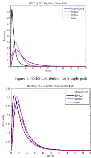
In the general tests, the position only covariance NEES values produced distributions drastically different than the expected chi-squared distribution. The distribution produced by the kinematic confidence estimates were much closer to a chi-squared distribution but still did not regularly follow the ideal distribution expected. When the algorithms were tested with simple paths, the NEES distribution would regularly spike in between NEES values between zero and four far above the ideal distribution and quickly drop to zero with a small right tail. The NEES distribution can be seen in Figure 1. This result showed a regular under confidence for all three algorithms tested, particularly the BDNLO which was consistently under confident for simple path estimations. Although the KMAVNLOCI and the BDMod appeared to create a regularly under confident distribution, NEES values under one were rarely produced reflecting the effect of the uncorrected sensor bias.
The NEES values were drastically different for the complicated path trials. The initial spike still existed but was closer to the ideal distribution. The NEES distribution contained a long right tail showing an increased amount of over confident trials, particularly when only the position covariance was used to create the confidence estimate. The right tail diminished drastically once the kinematic covariance was implemented. The resulting NEES distributions for each algorithm can be seen in Figure 2 juxtaposed over the ideal chi-squared distribution with three degrees of freedom. The KMAVNLOCI and the BDMod distributions still appear to be shifted right from the uncorrected bias but contain less significant right tails closer or under the ideal distribution. The BDNLO appeared to have corrected the simulated sensor bias but has a larger probability of creating over confident estimates.
that trial will be under confident; otherwise each estimate becomes significantly more over confident.
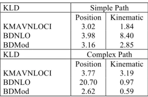
The Kullback-Leibler Divergence (KLD) is another effective way of determining how well the current model accurately represents the statistical characteristics of a system. The KLD measures the amount of information lost by using one model to describe a process. In this case, the statistical model would be the multi-variate Gaussian metric used to calculate positional confidence and the process is the actual error function created when using the NLO algorithms described in this paper. Below in Table 1 is the KLD metrics for the different algorithms for the NEES values created by only using the position covariance matrix and NEES values created by using all kinematic elements in the covariance matrix as described in (5). Using the full Kinematic covariance improves the performance of the model in every case except the BDNLO algorithm on the simple path. This occurs because the BDNLO is already creating under confident estimates and then creating even larger confidence regions to account for acceleration and velocity covariance. The model will continue to be very under confident especially for the bias-drift methods until the confidence of the sensor bias-drift estimation functions is accounted for in the final sensor covariance used in the position confidence estimation. On the other hand, as soon as acceleration and velocity becomes more irregular and harder to track such as in the complex path tests, the kinematic estimation model performs much better than the position estimation model (Kullback, 1951, Hershey 2007).
KLD Simple Path
Position Kinematic
KMAVNLOCI 3.02 1.84
BDNLO 3.98 8.40
BDMod 3.16 2.85
KLD Complex Path
Position Kinematic
KMAVNLOCI 3.77 3.19
BDNLO 20.70 0.97
BDMod 2.62 0.59
Table 1. Kulback Leibler Divergence Values 4.3 Algorithm Limits
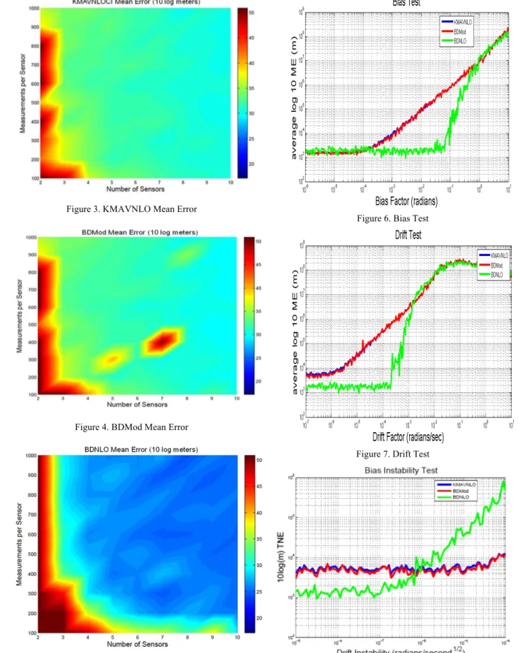
One of the controlled tests revealed one of the significant limits of the BDNLO compared to the KMAVNLOCI and the BDMod algorithms. At low numbers of sensors and measurements per sensor, the BDNLO is extremely likely to produce inaccurate measurements and diverge. This is likely caused by the lack of measurements and sensor reference points in order to converge on a steady sensor bias-drift state. The mean error of each of the algorithms from that particular test on a set of complicated paths can be seen in Figures 3-5. If there are only two sensors, the BDNLO is expected to diverge. For a complicated path, this effect exists in the other algorithms but is not guaranteed. When this test was repeated on simple paths, the KMAVNLOCI and BDMod regularly converged at two sensors at a slightly less accurate estimate but the BDNLO continued to diverge. The BDNLO appeared to be more easily affected when measurements per sensor are lower as well. As seen in Figures 3-5. Once an adequate amount of measurements are made on enough platforms, the BDNLO appears to perform regularly. Another test for the three algorithms revealed the effect of increasing and decreasing the different error simulation elements on the three different algorithms. As seen in Figure 6, once the initial sensor biases are as high as 100 micro radians, the KMAVNLOCI and BDMod algorithms begin to steadily
decrease in accuracy. The BDNLO has a high variation in performance at any instant but appears to perform relatively the same until maximum initial biases of 40 milli-radians. At this moment, the initial guess becomes so inaccurate that the BDNLO cannot converge. Similar results were found in the drift test shown in Figure 7 where the KMAVNLOCI and BDMod performance began decreasing at a maximum 1 micro radian per second and the BDNLO maintained constant performance until the maximum drift factor reached 0.2 milli-radians per second.
The last control test presented in Figure 8 shows the affect of increasing the drift instability has on the different algorithms. In this test the BDMod and the KMAVNLOCI performed more resistant than the BDNLO which began seeing increasingly degraded performance around 0.1 micro radians per second1/ 2. There is a point where the zero mean element of the IMU random walk can prevent the BDNLO from converging. Regardless of the spectrum of bias instability tested, the BDMod algorithm continued to improve the KMAVNLOCI on a regular basis.
It is important to keep all of these parameters in mind when choosing an algorithm with a particular system. If IMUs in a system are accurate enough, including the bias drift elements in the NLO algorithm only creates more performance variance. The BDMod method, though not as significant of a modifier, contains very little risk for such systems containing higher end IMUs.
5. CONCLUSION
5.1 Algorithm Improvement
The two modifications to the KMAVNLOCI have very different performance affects. The BDMod marginally improves accuracy but contains extremely little risk of significantly hurting performance while the BDNLO significantly improves accuracy of the KMAVNLOCI at a more significant risk of hurting performance. The BDNLO does appear to perform much more regularly as path types become much more simplistic or more information is included from more sensors. The BDNLO works in a much more specific window than the other two algorithms.
These algorithms are practical for any type of remote sensing platforms where LOS measurements are collected. Now that unknown multi-sensor bias and drift can be corrected, LOS localization applications can be used on a larger variety of sensing systems where the IMU drift has previously been too significant to accurately track an object. Pointing accuracy is the largest component impeding AOA localization applications and now it can be done with much cheaper IMUs.
5.2 Future Work
The development of these NLO algorithms has been in a MATLAB environment and the algorithms are still too slow to be implemented in a real-time environment. The most computationally intense operations include creating large matrices in set up and more significantly calculating the change in state during each NLO iterative step. Each change in state calculation inverts and multiplies matrices which grow quickly as more and more measurements are included in the trial. The algorithm has plenty of room to be speed up by implementing the method in a fast lower level language and optimizing the matrix operations either in code or on a GPU array.
REFERENCES
Hartley, Richard and Zisserman, Andrew. 2000. Multiple View Geometry in Computer Vision. Cambridge University Press, ISBN: 0521623049.
S. Hartzell, L. Burchett, R. Martin, C. Taylor, and A. Terzuoli, 2015. Geo-location of Fast-moving Objects from Satellite-based Angle-of-Arrival Measurements. IEEE Journal of Selected Topics in Applied Earth Observations and Remote Sensing, v.8(7).
J.R. Hershey and P.A. Olsen. “Approximating the Kullback Leibler Divergence Between Gaussian Mixture Models”. In: Acoustics, Speech and Signal Processing. IEEE International Conference on. Vol. 4. 2007, pp. IV–317–IV–320. DOI: 10.1109/ICASSP.2007.366913.
Julier, S.J. and Uhlmann, J.K.. 1997. A non-divergent estimation algorithm in the presence of unknown correlations. In: American Control Conference, 1997. Proceedings of the 1997. Vol. 4. 1997, pp. 2369–2373 vol.4.
Kaplan, Elliott D. 2005. Understanding GPS: Principles and Applications, Second Edition. Artech House. ISBN: 1580538940.
Woodman. Oliver J., An introduction to inertial navigation. 2007.
Sprang, J, D. Hesser, J. Roos, J. Mautz, M. Sambora, C. Taylor, J. Sugrue, A. Terzuoli, 2015, “CORRELATED ERROR ANALYSIS FOR THE NON-LINEAR OPTIMIZATION AOA GEOLOCATION ALGORITHM,” Proceedings of the 2015 IEEE International Geoscience and Remote Sensing Symposium (IGARSS 2015), Milano, IT, 26-31 July 2015. Rong Li, X., Zhao, Z., and Jilkov, Vesselin P. . 2001. Practical Measures and Test for Credibility of an Estimator. Proc. Workshop on Estimation, Tracking, and Fusion—A Tribute to Yaakov Bar-Shalom. 2001.
Wu, A. 1998. SBIRS high payload LOS attitude determination and calibration. In: Aerospace Conference, 1998 IEEE. Vol. 5. 1998, 243–253 vol.5.
Yang, B. and Scheuing, J. 2005. Cramer-Rao bound and optimum sensor array for source localization from time differences of arrival. In: Acoustics, Speech, and Signal Processing, 2005. Proceedings. (ICASSP ’05). IEEE
International Conference on. Vol. 4. 2005, iv/961–iv/964 Vol. 4. S. Kullback and R. A. Leibler. “On Information and
Sufficiency”. In: Ann. Math. Statist. 22.1 (Mar. 1951), pp. 79–
86. DOI: 10.1214/aoms/1177729694. URL: http://dx.doi.org/10.1214/aoms/1177729694.
J.R. Hershey and P.A. Olsen. “Approximating the Kullback Leibler Divergence Between Gaussian Mixture Models”. In: Acoustics, Speech and Signal Processing. IEEE International Conference on. Vol. 4. 2007, pp. IV–317–IV–320. DOI: 10.1109/ICASSP.2007.366913.
Figure 1. NEES distribution for Simple path
Figure 3. KMAVNLO Mean Error
Figure 4. BDMod Mean Error
Figure 5. BDNLO Mean Error
Figure 6. Bias Test
Figure 7. Drift Test