Forecasting Social Unrest Using Activity
Cascades
Jose Cadena1,2*, Gizem Korkmaz1, Chris J. Kuhlman1, Achla Marathe1,3, Naren Ramakrishnan2, Anil Vullikanti1,2
1Virginia Bioinformatics Institute, Virginia Tech, Blacksburg, VA, USA,2Department of Computer Science, Virginia Tech, Blacksburg, VA, USA,3Department of Agricultural and Applied Economics, Virginia Tech, Blacksburg, VA, USA
Abstract
Social unrest is endemic in many societies, and recent news has drawn attention to happen-ings in Latin America, the Middle East, and Eastern Europe. Civilian populations mobilize, sometimes spontaneously and sometimes in an organized manner, to raise awareness of key issues or to demand changes in governing or other organizational structures. It is of key interest to social scientists and policy makers to forecast civil unrest using indicators ob-served on media such as Twitter, news, and blogs. We present an event forecasting model using a notion of activity cascades in Twitter (proposed by Gonzalez-Bailon et al., 2011) to predict the occurrence of protests in three countries of Latin America: Brazil, Mexico, and Venezuela. The basic assumption is that the emergence of a suitably detected activity cas-cade is a precursor or a surrogate to a real protest event that will happen“on the ground.” Our model supports the theoretical characterization of large cascades using spectral prop-erties and uses propprop-erties of detected cascades to forecast events. Experimental results on many datasets, including the recent June 2013 protests in Brazil, demonstrate the effective-ness of our approach.
1 Introduction
Social media has become a window into happenings on the ground, from earthquakes [1] to specific news stories [2]. A key population-level event is civil unrest, i.e., protests, strikes, and occupy events, wherein civilian populations mobilize to raise awareness of key issues. As is evi-dent from recent protests in many countries (e.g., Egypt, Turkey, Brazil), social media plays an important role in documenting, triggering, mobilizing, or even quelling such events, e.g., see [3,
4]. However, it is not clear when preliminary chatter observed on social media becomes a true precursor for a protest, and thus understanding the structure of the tweet behavior is a relevant problem.
While Twitter is used for many purposes (e.g., discontent expression, event reporting, planned protest recruitment), all of which can be used in a predictive model for civil unrest, we a11111
OPEN ACCESS
Citation:Cadena J, Korkmaz G, Kuhlman CJ, Marathe A, Ramakrishnan N, Vullikanti A (2015) Forecasting Social Unrest Using Activity Cascades. PLoS ONE 10(6): e0128879. doi:10.1371/journal. pone.0128879
Academic Editor:Tobias Preis, University of Warwick, UNITED KINGDOM
Received:May 25, 2014
Accepted:May 4, 2015
Published:June 19, 2015
Copyright:© 2015 Cadena et al. This is an open access article distributed under the terms of the
Creative Commons Attribution License, which permits unrestricted use, distribution, and reproduction in any medium, provided the original author and source are credited.
Data Availability Statement:Relevant data are within the Supporting Information files.
civil unrest forecasting. Our goal is to design a model that forecasts the date of the event. Cas-cades, as is well known, help formalize the spread of influence and information, e.g., see [8–
12]. Informally, cascades are subgraphs (often trees) that capture the spread of influence from a node to its newly activated/influenced neighbors and descendants.
There are many notions of cascades, which afford varying levels of formal characterization and utility. For instance, in Bakshy et al. [8], an edgeA!Bis included in a cascade only if it can be argued that some action (e.g., a posting or use of a URL) byBcan be directly attributed toA, which makes the analysis intensive in terms of data and computation; also, the mathemat-ical analysis under their model becomes challenging. Another common approach is to define cascades in terms of the (random) subgraph over which diffusion processes like linear thresh-old and independent cascades models spread, e.g. [12,13]. Here, we use a simpler notion of cascades (referred to as“activity cascades”), introduced by [5–7]. Informally, such a cascade consists of a tweet emitted by a useru, and the tweets of the users who see/mentionu’s message (for instance, her direct followers or users who mention her) given that those tweets are sent within a small time interval (denoted byΔ), and so on (see Section 3.1 for a precise definition). This turns out to be a special case of Hawkes processes [14–16], which are based on mixtures of mutually exciting point processes. Although simpler to define, we demonstrate that this no-tion of cascades has good predictive power for modeling civil unrest, and is also amenable to rigorous analysis. Our key contributions are focused on the following three questions:
1. When do large activity cascades happen?A common empirical observation is that cas-cades seldom become very large. We rigorously prove necessary and sufficient conditions for large cascades in terms of spectral properties of the underlying graph (Section 3.2); these also imply a similar characterization for a class of Hawkes processes. We find that this characteriza-tion closely matches our empirical observacharacteriza-tions for synthetic traces. Specifically, our analyses show if the spectral radius of a cascade graph (defined in Section 3.2) is below a particular con-stant, then large cascades are not possible. Our techniques build on approaches for analyzing the spread of epidemics [17–19], and are thefirst such resultsfor cascades of this kind.
2. Are there critical subsets of users that contribute to cascades?We study the questions of identifying critical subsets of users responsible for formation and survival of cascades, and formalize these as two complementary problems: CRITICALSETFORMATION(CSFP) and C RITICAL-SETSHATTERING(CSSP). We show both to be NP-complete, and we evaluate different greedy heuristics to approximate them empirically by studying large, monthly cascades for all (coun-try, month) combinations for Brazil, Mexico, and Venezuela over a 15-month period. Our re-sults for CSSP show that a very small set of users are critical for a cascade to exist—their non-participation causes the cascade to shatter. We also prove that a high degree strategy gives a constant factor approximation for CSSP in random power law graphs. On the other hand, the results for CSFP suggest that unless a large fraction of users participate a cascade cannot exist. Thus, one needs a reasonable fraction of users, plus some critical users for a cascade to exist. These are validated through empirical observations in Section 4.2.
3. Can we forecast protests using activity cascades?Since large cascades are not very com-mon, their occurrence signals a big event. We analyze over 353 million tweets from three Latin American countries over a 1.5-year period, and consider activity cascades formed by a filtered set of tweets. These tweets contain at least 3 keywords from a dictionary that has over 900 words in English, Spanish and Portuguese, related to civil unrest activities. This ensures that the resulting activity cascades will be relevant to the topic of civil unrest. Next, we build a fea-ture set based on the structural properties of the cascades, to be used as predictors of social un-rest. Statistical models are then used to remove redundancies among features and make predictions of events from the reduced feature set. The model is tested on multiple countries for robustness and compared against a baseline model. We show that our approach can‘beat
Foundation (NSF) under grant number CCF-1216000 and NSF grant number CNS-1011769. The US Government is authorized to reproduce and distribute reprints of this work for Governmental purposes notwithstanding any copyright annotation thereon. Disclaimer: The views and conclusions contained herein are those of the authors and should not be interpreted as necessarily representing the official policies or endorsements, either expressed or implied, of IARPA, DoI/NBC, or the US Government. None of the funders or grants represent commercial funding sources, since they are all US federal agencies.
the news,’i.e., contribute a lead time of one to two days over the reporting of a protest in major news media, with an accuracy of over 0.75. It can even predict black swan events like the Brazil-ian Spring with an accuracy of 0.83. (Section 4.6).
Our paper helps explain the model and observations of [5–7] rigorously, especially condi-tions for occurrence of large cascades. Since their frequency is relatively low, their occurrence is a signal of significant events—-this corroborates with the observations of [5], and is the basis of our approach for forecasting protest events.
1.1 Related work
Analyzing traffic trends in twitter and other social media sites is a very active topic of research. Some of the specific applications include identifying specific news stories [2,20], tracking natu-ral disasters [1], predicting stock market moves [21,22] and understanding political or cultural events [5,6,23,24]. Yang et al. [25] predict temporal patterns in the usage of specific hashtags in social media data. Hutto et al. [26] show that increases in followers on Twitter are predicated on social behavior, message content, and social network structure variables in roughly equal proportions. Hsieh et. al. [27] demonstrated that experts could not match the crowd in identi-fying future interesting news stories. Most of these works have focused on counts of keywords and hashtags, and do not capture peer influence in the use of such terms. Peer influence is often modeled by diffusion processes, such as linear threshold and SI/SIS/SIR epidemic models, e.g., [12,13]; in this context, cascades are used to refer to the (random) subgraph on which the diffusion spreads. There has also been a lot of work on using semantic information for attribut-ing influence more carefully, e.g., [8–11], as discussed in Section 1.
A simpler notion of cascades is studied by [5,6] in Twitter follower graphs and by [7] in the mentions graphs. Large cascades involving protest-related hashtags are found to occur infre-quently. Our formulations extend point process models, which have been studied extensively. Two closely related approaches are by [15,16]. Simma et al. [15] consider a model in which a Poisson process triggers other Poisson processes. They develop an EM algorithm to infer the random forest of events, which captures the cause of each event. Zhou et al. [16] use a multi-di-mensional Hawkes process.
There are other works that utilize models for characterization and prediction. Linear regres-sion models using average tweet rates, and tweet rate time series (per-day tweet rates over a 7-day period), have been used to predict box-office revenues from movies [28]. A classifier and hidden Markov model have been used with tweet content to establish the onset and end of identified events (versus event prediction) [29]. Natural language processing and LDA have been used to identify topics that capture collections of events identified in tweets; a linear re-gression model is then used to predict crimes [30].
With respect to forecasting social unrest, [31] provides empirical data showing that in-creases in food prices correlate with protests in 2008 and 2011. Rather than predicting specific unrest events, [32] uses a 2-parameter dynamics model to predict the distributions of numbers of unrest events per year, for many regions of the world. Disease outbreaks, deaths, and riots are forecasted with topic detection and tracking using news articles, and a Bayes scheme to compute the probability of some event, given other events occurring beforehand [33]. A ten-sion parameter, based on hashtag usage, was shown to correlate well with clashes in Egypt be-tween secularists and Islamists [34]. A generalized least squares model of politicalviolence[35] is used to predict the overall level of violent activity in a country, by year. By contrast, we are in-terested in violent and non-violent protests.
an SIS process; our analysis strongly builds on this approach, but our model requires the use of a variant of the node expansion, instead of edge expansion. Similar spectral radius bounds are also considered in [18,19] for the SIS process.
Our work can be differentiated from the above studies in the following ways. This is the first work of which we are aware that predicts daily civil unrest events in multiple countries using a combination of different graph cascade characteristics. Further, we explain theoretically and demonstrate empirically conditions that delineate small and large cascade regimes, using spec-tral properties of the underlying graphs.
2 Materials
2.1 Twitter Dataset
For event prediction, we use a set of over 353 million tweets collected for Brazil, Mexico and Venezuela for the period of May 2012 through November 2013. Our dataset constitutes a 10% sample of the tweets for these countries during the above time period.
Our analysis is done separately for each country, and, as a pre-processing step, the tweets are filtered by country (using geolocation codes, place identifiers, language detection, author identification, and other enrichment processes), ignoring tweets for which a country of origin could not be determined. Next, we organized a vocabulary of 614 protest-related words (such as march, riot, strike, organize, democracia, conflicto, revolucion, criminalidade), 192 key-phrases (such as“right to work”,“marcha por la paz”), and 105 country-specific key players (which include important public figures, political parties, labor unions), collectively referred to henceforth as keywords. Compiled by social scientists who are experts in the region, the key-words include English, Spanish, and Portuguese translations. We then subselect tweets which contain at least 3 keywords from our vocabulary. Tweet volumes before and after filtering are shown inTable 1.
2.2 Follower Data
We obtained the follower network for a subset of the users who appear as authors in our data-set, for each country by using Twitter API from a large number of machines. The size of the graphs for the three countries are the following: Mexico has 79,598 nodes and 1,437,687 edges, Venezuela has 312,241 nodes and 21,119,120 edges, and Brazil has 142,176 nodes and
6,854,368 edges.
2.3 Gold Standard Report (GSR) Datasets
GSR datasets are compiled by an independent group, selected by IARPA (Intelligence Ad-vanced Research Projects Activity), which is comprised of social scientists and experts on Latin America. A small set of well-reputed newspapers for each country are used to identify the in-stances of civil unrest events to be included in the GSR. For each event, the GSR captures the
Table 1. Number of tweets for the period May 2012 to Nov 2013.
Country Raw Filtered
Mexico 97,873,616 3,524,695
Venezuela 105,938,438 6,683,834
Brazil 150,147,141 1,575,041
when, where, who and why of the event, i.e. the date of the event, its geographic location, the population protesting (e.g. labor, medical workers, general population) and the reason for the protest (i.e., the event type, e.g., economic, political, resource). Here we are interested in fore-casting primarily the if/when of the event (although text classification and geo-coding of the tweets reveals insight into where/who/why, something we do not study here further).
3 Methods
3.1 Activity Cascades
LetG= (V,E) denote a directed graph, withNo(u) andNin(u) denoting the set of out-neighbors and in-neighbors for a nodeu2V, respectively. The nodes represent Twitter users. We consider two kinds of graphs—afollowergraph and a combinedmentionsandretweetgraph. An edge (u,v) has different interpretations depending on the graph, as discussed below. We assume each userusends at most one tweet at a time (with one second granularity), so a node-time pair (u,t) identifies a tweet. For a nodeu2V, timetand time intervalΔ, we define a cascadeC (u,t,Δ) to be a set of tweets/node-time pairs in the following recursive manner, using the for-mulation of [5–7].
• If there is no tweetdriven bynodeuat timet, thenC(u,t,Δ) =ϕ.
• Else,C(u,t,Δ) = {(u,t)}[{x2C(v,t0,Δ):v2N
o(u),t02(t,t+Δ]}
The termdriven bywill be explained below. This general notion of cascade makes no prior assumptions about the nature of the edges connecting the nodes of the graph, which gives us the flexibility to define the neighborhood of a node in different ways. Though this definition does not explicitly look for any correlation between the messages ofuandv(which is used by, e.g., [8–12]), we use it on a set of tweets that are already filtered for protest related keywords, as done by [5–7], which brings in some correlation. Also, note that this notion of cascades is dif-ferent from the more commonly studied notion associated with diffusion processes, e.g., [12,
13]—here, a cascade is a random subgraph on which the influence spreads.
In this paper, we study two types of activity cascades:follower(F) and combinedmention
plusretweet(MRT) cascades, defined, respectively, by thefollowerandmentionandretweet
graphs, each of which models a different kind of interaction between users in the Twitter net-work. Our methodology is the same as [36], except that we also include retweets.
In a follower graph, for every nodeu2G,No(u) is the set of Twitter followers ofu, and
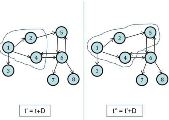
Nin(u) is the set of Twitter friends ofu(i.e. users followed byu). From this definition, follower cascades in Twitter emerge in the following manner: a useruposts a tweet at timetstarting a cascade where she is the only participant. For each followervofuwho posts a tweet at some timet02(t,t+Δ], (v,t0) is added to this cascade, and so on, as illustrated inFig 1. This process is repeated until no more users can be added to the cascade.
We combine mentions and retweets to form an MRT graph because both types of tweets in-dicate influence between pairs of users. Suppose a userwwith nameWcomposes a tweet at timet1that mentions another useruwith nameU, whereWandUare sequences of characters
of the form[a−zA−z0−9_]+. In the following, we specify the concatenation of two
influencesx. If the two tweets occur such thatt22(t1,t1+Δ], then the two edges link up to form
a directed path of length 3,u!w!x, and the cascadeC(u,t1,Δ) = {(u,t1), (w,t2)}.
We have several notes. The termdriven byindicates the user that instigates the cascade. For a follower graph, the instigator is the user that sends the first tweet of a cascade. For an MRT graph, the instigator is the first influencer of a cascade. Second, users (nodes) in an MRT graph with zero out-degree (xin this example) are not included in the MRT cascade because there is no evidence that these nodes influence other users. Also, a single tweet can produce multiple edges in an MRT graph. Since retweets of an original tweet preserve the original tweeter, no matter how many times the original tweet is (sequentially) retweeted, a set of these retweets (without mentions) produces a star subgraph of the MRT graph. Finally, MRT cascades, unlike follower cascades, directly use tweet payloads; however, F cascades utilize the follower graph.
We provide additional definitions that will be useful in forecasting social unrest. We say that a (follower or mentions/retweet) cascadeCisactiveon daydif there exists at least one message or tweet (u,t) by useruat timet, such thattis some time during daydand (u,t) is an element ofC. Thesizeof a cascade is the number of tweets comprising it. Auserorparticipant
is a tweeter.
3.2 Characterizing large cascades in terms of graph properties
Our empirical results suggest that large and long cascades are rare, and arise within communi-ties of users. We now attempt to explain this behavior by relating it to the spectral propercommuni-ties of the graph, by considering a formulation based on a slight relaxation of the notion of cascades: We consider a cascade starting at a random initial nodeu0at timet0; (i)X(0) denotes the initial
Fig 1. Formation of cascades in the Twitter follower network.At timet, node 1 posts a tweet. Nodes 2 and 4 post at timest2andt4betweentandt0=t+D. Node 5, which follows 2, posts at some timet5between t0andt@=t0+D. Therefore, the cascadeC(1,t,D) isC(1,t,D) = {(1,t), (2,t2), (4,t4), (5,t5)}.
configuration. We say that (u0,t0) is active in the cascade at timet0. Following our definition,
we will think of a cascade as consisting of tweets indexed by user-time pairs (u,t); (ii) The number of tweets sent by each useruis a Poisson process with parameterαu; (iii) If useru sends a message at timet, and some other uservwithu2No(v) is active at timet, then (u,t) be-comes active in the cascade at timet; (iv) A tweet (u,t) ceases to be active after a (random) time durationD(u,t) drawn from an exponential distribution with parameterδ= 1/Δ; and (v) The cascadeC(u0,t0) dies when there are no more active tweets in it.
We now model this as a Markov processX(t)with values inNV. LetXu(t) denote the
num-ber of messages by useruthat are active at timet. Then, the cascade evolves in the following manner:
Xu: increases by 1 at rate aðuÞ if fv2NinðuÞ:Xv>0g 6¼ ð1Þ
Xu: decreases by 1 at rate dXu ð2Þ
Every cascade eventually becomes inactive, sinceXu= 0 for alluis the unique absorbing state for this Markov process. Thelifetimeof the cascade, the duration for which it lasts, is pre-ciselyT= sup{t:Xu(t)>0,for someu2V}. We now derive necessary and sufficient conditions for obtaining large cascades.
3.2.1 Multivariate Hawkes Processes. Our formulation above makes it a special case of the multivariate Hawkes processes, as we now discuss. A Hawkes processNtis a type of
self-ex-citing counting process characterized by a time-dependent intensity (rate)λ(t) [14–16]. LetNd(t)be a multidimensional counting process, whered2{1,. . .,D} denotes a dimension
(withDbeing the number of dimensions). Letλd(t) denote the intensity ofNd(t). The process is defined in the following manner:
ldðtÞ ¼mdðtÞ þX D
d0¼1
Z t
1
kd0dðt sÞdNd0ðsÞ;
whereμdis a base intensity for dimensiond, andκd0d(τ) is a kernel function describing the
in-fluence of the previous events in dimensiond0on the current rate ond.
For our formulation, let each nodeu2Vbe a separate dimension, and letNu(t)be the
num-ber of messages contributed to an ongoing cascade. We haveμu(t) = 0 and the kernel function asκvu(τ) =αvu×κ(τ), where: (i)αvu=αuNv(t) ifv2Nin(u); otherwise,αvu= 0. Here,αuis the (fixed) tweeting rate ofu, andαvudescribes the fact thatu’s contributions to the cascade are proportional to her in-neighbors’contributions (i.e. her friends in the follower graph); and (ii)
κ(τ) = 1 if 0<τΔ; otherwiseκ(τ) = 0. As a result, we have:
luðtÞ ¼aðuÞ X v2NinðuÞ
ðNvðtÞ Nvðt DÞÞ
We use the processX(t)below for our discussion, since it simplifies the analysis; our results hold for a class of Hawkes processes with the kind of kernel function mentioned above.
3.2.2 Conditions for Small Cascades. We now derive conditions when the maximum cas-cade size isO(logn), with high probability, wherenis the number of nodes. The processX(t)is non-linear, making it quite complex to analyze; instead we consider the following relaxation
Y(t):
Yu: increases by 1 at rate aðuÞ
P
Yu: decreases by 1 at rate dYu ð4Þ
Lemma 1The processY(t)stochastically dominatesX(t)so thatX(t)Y(t)for all t0.
Proof 1Our proof is based on designing a coupling that ensures thatX(t)Y(t) for all
t0, and builds on [17]. Clearly,X(0)Y(0). We consider the processY(t)and for each node
u, we sample random variablesR1 uandR
2
ufrom exponential distributions with parameters α(u)∑v2N
in(u)YvandδYu, respectively. The first transition out ofY(0) happens at timeτ, which
equals minufR 1 u;R
2
ug. Our coupling will specify the transition for the processX(t)in the
follow-ing manner. Suppose the transition at timeτcorresponds toYu(τ) =Yu(0) + 1; this would have happened with rateα(u)∑v2N
in(u)Yv(0). For the corresponding processX(t), the transition Xu(τ) =Xu(0)+1 is made with probability
1
P
v2NinðuÞYvð0Þ
, if {v2Nin(u):Xv>0}6¼ϕ; otherwise
Xu(τ) =Xu(0). This ensures that the transitionXu(τ) =Xu(0)+1 happens with the correct rate. Similarly, the transition corresponding toYu(τ) =Yu(0)−1 can be handled to get a coupling of the first jumps inX(t)andY(t).
Lemma 2Letρ(A) denote the spectral radius ofA, the adjacency matrix ofG. Assume that
Gis a bi-directed graph and letαmax= maxuα(u). Ifαmaxρ(A)<δ, the duration of the cascade
Tsatisfies Pr[T>t]ne−(δ−αmaxρ(A))tandE½T lognþ1 d amaxrðAÞ.
Proof 2Our proof is an adaptation of that of [17] for the SIS model; we describe it here completely for completeness. From equations (3, eqn:y2), it follows that
E½YuðtþdtÞ YuðtÞjYðtÞ ¼ aðuÞ
X
v2NinðuÞ
YvðtÞdt dYuðtÞdtþoðdtÞ
amax X
v2NinðuÞ
YvðtÞdt dYuðtÞdtþoðdtÞ;
which impliesdE½YðtÞ
dt ðamaxA dIÞE½YðtÞ.
This has solutionE[Y(t)]e(αmaxA−δI)Y(0). From Lemma 1, and sinceX(0) =Y(0), we have E[X(t)]e(αmaxA−δI)X(0).
LetNt=∑vXv(t) =1TX(t) denote the number of nodes infected at timet. Then,Nt1T
e(αmaxA−δI)X(0). SinceAis a symmetric matrix,e(αmaxA−δI)is also symmetric, and we have keðamaxA dIÞXð0Þ krðeðamaxA dIÞÞ kXð0Þ k¼eamaxrðAÞ dpffiffiffin. This impliesE[N
t]neαmaxρ(A)−δ=
ne−(δ−αmaxρ(A)), sincekXð0Þ k ffiffiffi
n p
. The first part of the lemma follows since Pr[T>t] = Pr [Nt1]E[Nt].
For the second part of the lemma, we have
E½T ¼
Z 1
0
Pr½T>tdt
Z 1
0
minf1;neamaxrðAÞ dg
Z logn=ðd arðAÞÞ
0
1dtþ
Z 1
logn=ðd amaxrðAÞÞ
ne ðd amaxrðAÞÞdt
lognþ1
d amaxrðAÞ
3.2.3 Conditions for Large Cascades. We now consider the conditions for having a large cascade (of sizecm, wherecis a constant larger than 1, andmis a parameter). We need the fol-lowing version of the isoperimetric constant, which captures node expansion.
^
ZðG;mÞ ¼ min
SV;jSjm
P
v2V S:NinðvÞ\S6¼av
jSj :
We sometimes omit the reference to the graphGin^ZðG;mÞ, and just useZ^ðmÞwhenGis
clear from the context. We now consider a Markov processZ(t) with state space {0,. . .,m},
de-fined in the following manner:
ZðtÞ ¼ ZðtÞ þ1 at rate ^ZðmÞZ; if Z<m ZðtÞ ¼ ZðtÞ 1 at rate dZ; if Z>0
Lemma 3Z(t) is stochastically dominated by∑uXu(t), i.e.,Z(t)∑uXu(t) for allt0.
Proof 3The proof is also by designing a coupling, as in Lemma 1. We assume thatZ(0) ∑uXu(0), and prove the statement by induction. We consider the processX(t) and for each nodeu, we sample random variablesR1
uandR 2
ufrom exponential distributions with parameters α(u)1{v2Nin(u):Xv>0}6¼ϕandδXu(0), respectively. The first transition out ofX(0) happens at
timeτ, which equals minufR 1 u;R
2
ug. Our coupling will specify the transition for the processZ(t)
in the following manner. LetS= {w:Xw(0)>0}. LetN+(S) = {v2V−S:N(v)\S6¼ϕ}.
Suppose the transition at timeτcorresponds to a transitionXu(τ) =Xu(0)+1 for some node
u(which increases the number of active messages). The total rate at which such an increase happens equals∑uα(u)1{v2Nin(u):Xv>0}6¼ϕ=∑u2N+(S)α(u). First, suppose thatjSj<m. The
transitionZ=Z+1 is now made at timeτwith probability
^
ZðmÞZ
P
u2NþðSÞaðuÞ
:
This fraction is in [0, 1], becauseZð0ÞZ^ðmÞ P
u2NþðSÞaðuÞ, by definition of^ZðmÞ, and because
jSj<m, so that the transition happens with the correct rate. Second, ifjSj m,Zis unchanged, which is the correct rate.
Next, we consider the case that the transition at timeτcorresponds to a transitionXu(τ) =
Xu(0)−1 = 0 for some nodeu. In this case, the transitionZ(τ) =Z(0)−1 is made with probability
Zð0Þ
P uXuð
0Þ, which is well defined since this is in [0, 1]. Also, note that there is some probability
that∑uXu(0) decreases by 1, butZ(0) does not—this does not violate the property, because in
this caseZ(0)<∑uXu(0).
Therefore, in either case, we haveZ(τ)∑uXu(τ), and the lemma follows.
Lemma 4Supposer¼ d ^
ZðmÞ<1. Then, we have Pr½T>
r mþ1
2m 1 r
e ð1þOðr mÞÞ.
Then, we have:
pði;iþ1Þ ¼ ^ZðmÞ ^
ZðmÞ þd; i¼1; ;m 1;
pði;i 1Þ ¼ d ^
ZðmÞ þd; i¼1; ;m 1
pð0;0Þ ¼ 1; pðm;m 1Þ ¼ 1:
Then, the duration of the cascade,T, is the time before the process hits 0. As in [17], this is the standard gambler’s ruin probability, and the rest of the proof follows exactly as in [17].
Spectral connection. Vertex expansion is related to the graph spectrum. IfGis ad-regular graph, and if its spectral gap, i.e., the difference between the smallest and second smallest eigen-value, isμ, the vertex expansion for sets of size at mostmis 1
ð1 m=nÞm2
þm=n.
3.2.4 Identifying Critical Sets in a Cascade. We now consider the following questions: What is the critical subset of users whose tweets are responsible for the cascade to survive? What is the critical subset of users whose removal would cause the cascade to disintegrate? These are related and complementary problems, which can help explain the conditions for cas-cade formation. We consider a slightly more general notion of cascas-cades than the one defined in Section 3.1—for a setSof nodes, we defineC(S,t,Δ) =[u2SC(u,t,Δ) to be the union of cas-cades starting at nodes inS. As a result, any directed acyclic graph can be seen as a cascade formed by its sources.
CRITICALSETSHATTERINGProblem CSSP(G,C,k):
Input: A set of cascadesCin a graphG= (V,E) and parameterk.
Goal: Determine the smallest setSVof users, such that the sub-cascades of allC2CinG
[V\S] are of size at mostk.
Thus, the goal in CSSP is to find the subsetSwhose removal causes all cascades inCto be “shattered”.
CRITICALSETFORMATIONProblem, CSFP(G,C,α,k):
Input: A set of cascadesCin a graphG= (V,E), tweet rateαand parameterk.
Goal: Determine the smallest setSVof users, such that for everyC2C, a sub-cascade of
size at leastkexists in the graphG[S] with tweet rateα.
Thus, CSFP quantifies the number of users needed to cause large cascades. While CSSP and CSFP are closely related and seem to be complementary problems, they are quite different from a computational perspective.
Complexity and algorithms for CSSP. We have the following result.
Lemma 5CSSP (C,G,k) is NP-complete.
Proof 5It is easy to verify that CSSP is in NP. The NP-hardness of CSSP is by a reduction from the balanced graph partitioning problem (see, e.g., [37])—this problem involves finding the smallest subsetSV0of nodes in an undirected graphH= (V0,E0) so that all components inH[V0−S] have size at mostb, which is a given parameter.
LetCbe a DAG formed by orienting the edges ofHarbitrarily, so that it forms a DAG. Let
Whenever the condition in Lemma 2 is tight, i.e., it gives both necessary and sufficient con-ditions, CSSP can be solved by simply attempting to reduce the spectral radiusρ(A). We con-sider the special case of the Chung-Lu random graph model [38]: given a weight sequencew= (w(v1),w(v2), ,w(vn)) for nodesvi2V, the random graphG2G(w) is obtained by choosing each edge (u,v) with probabilityPwðuÞwðvÞ
vi2VwðviÞ
. We use the following result from [39].
Lemma 6[39] IfG=G(w) is a random graph in the Chung-Lu model with the weight
se-quence being a power law with exponentβ>2,removal of theΘ(n/T2(β−1))nodes with the
high-est weight ensures that the spectral radius of the residual graph is at most T, almost surely. Motivated by Lemma 6, we study heuristics for CSSP based on degree and the core number in the underlying graph. SincerðAÞ ffiffiffiffiffiffiffiffiffiffiffiffiffiffiffiffiffiffiffiffiffiffiffiffiffiffiffiffi
maxvdegðv;GÞ
p
, a natural heuristic for CSSP is to re-duce the maximum degree maxvdeg(v,G). Also, sincerðAÞ
2jEðHÞj
jVðHÞjfor any subgraphHofG, another natural heuristic for CSSP is to reduce the density of every subgraphH. Motivated by these bounds on the spectral radius of a graph, we consider the following heuristics for CSSP: (i)high degree heuristic: remove nodes in decreasing order of degree inG; and (ii)high core number heuristic: remove nodes in decreasing order of their core-number inG.
Complexity and algorithms for CSFP. We have the following hardness result.
Lemma 7CSFP (C,G,α,k) is NP-complete.
Proof 7It is easy to verify that CSFP is in NP. We only discuss the NP-hardness. Our proof is by a reduction from the Set Cover problem, an instance of which consists of a setBof ele-ments, a setAof subsets ofB; the goal is to select the smallest subsetA0Asuch that each ele-ment inBis covered by a set inA0.
We construct an instance of CFP in the following manner. We setto be a large integer. We construct a graphG= ({r,r0}[A[B,E), whereEconsists of the following edges: edges (j,i) if
j2B,i2Aandjis contained in seti, edges (r,i), (r0,i) for alli2A, and edge (r,r0). We haveαr=
αr0=, whileαu= 1/nfor allu2A[B. We note thatZðG;^1;fugÞ for allu2{r,r0}[A.
SupposeA0Ais a minimum set cover. Then, increasingα
u=for allu2A0will ensure thatZðG;^1;fjgÞ for allj2B. Similarly, supposeSis the optimum solution to the CFP
prob-lem. Clearly,SA; ifS\{r,r0}6¼ϕ, we can dropr,r0fromSwithout affecting the feasibility of the solution. For eachj2B, there must be at least one neighbor inS; else, we cannot have
ZðG;^1;fjgÞ . This impliesSis a set cover.
This completes the reduction.
We consider a greedy algorithm for CSFP: pick nodes in non-increasing order of degree until the cascade on the graph induced by these nodes has size at leastk.
We note that the maximum cascade size can be estimated for a given rate assignment within a factor of 1 ±, with high probability, in timeO(jEjlogn/2) by a standard Chebyshev bound.
3.3 Forecasting Social Unrest using Cascades
Social media is believed to be responsible for facilitating critical communication often required to fuel momentum preceding the events of civil unrest. Here we explore the ability of Twitter data to act as a predictive signal of future civil unrest. Specifically, we study the prediction of civil unrest events (e.g., protests, strikes) by using properties of the activity cascades in Twitter data.
of future events of interest. These could be sport events, concerts, revolutions, elections, etc. However,given that our tweets are filtered by civil unrest related keywords, we expect the events detected will be of civil unrest type.
Starting from May 1, 2012 to November 30, 2013, each day, we compute the total number and size of cascades, number of participants and duration (in days) of cascades, change in the number of participants and tweets, average growth rate of tweets and average growth rate of participants. These features are collected daily for each active follower cascade and MRT cas-cade. For each of the features described above, we also compute the minimum, maximum, me-dian, and average of the cascade size, duration, and users, as well as the average value of the 1st, 2nd, 3rd, and 4th quartile of their distribution and add them to the feature set. Therefore, our initial feature set consists of 114 attributes: (7 cascade properties × 8 aggregate statistics × 2 types of cascades + (daily cascade count × 2 types of cascades)).
Our initial list of features is expected to be highly correlated, resulting in unstable estimates if used in regression modeling. For example, the cascade size of an MRT cascade is almost equivalent to the number of users in that cascade, since people tend to retweet a message only once. In addition, the majority of these cascades last for one day (duration = 1), which makes the average growth equivalent to the change in the cascade size on the last day, which in turn gives the change in the number of users, and so on.
In order to address the problem of multi-colinearity, we compute the correlation between every pair of features (i.e. the correlation matrix) and remove highly correlated features. Specif-ically, if the correlation between two variables is greater than 0.7, we only keep one of the two. This methodology reduced the size of our feature set from 114 to 13. Next, we use a regression methodology called LASSO (Least Absolute Shrinkage and Selection Operator) to further re-move the redundant features and to shrink coefficients [40]. The LASSO based logistic regres-sion model uses cascade features from both the follower and the MRT models.
3.3.1 Baseline model. We build a baseline model in order to set a benchmark and to mea-sure the added predictability provided by the Twitter data. The baseline model uses no external input in the regression model. It uses an autoregressive logistic model of order 1, since we have a binary dependent variable. It uses lagged values of itself as the predictor. Formally, we esti-mateYt=α+βYt−1+εwhereYtis the binary variable: 1, if there is an event on daytin the GSR; 0 otherwise. The fitted values ofYt, which give the likelihood of future events, are com-pared against the actual events in the GSR for measuring the model’s performance.
3.3.2 Evaluation metrics. Once the probabilities are estimated for the test days, a thresh-oldtis used to determine whether or not the probability exceedstfor an event to occur. The optimal thresholdtis determined by cross-validation, especially maximizing the area under the ROC (receiver operating characteristic) curve. Once learned,tis further used to separate events from non-events given the estimated probabilities. We evaluate our models against two settings—a lead time of 1 day and a lead time of 2 days—and compare the results against the GSR using standard measures such as precision, recall, and the misclassification rate.
4 Results and Discussion
Our experimental results are focused on answering the following questions.
1. Do our theoretical conditions for large cascades from Section 3.2 hold true in real datasets? (Section 4.1)
2. What level of increase in user tweeting initiates large cascades? Does the solution to the CFP problem using our greedy heuristic suggest that a few important users are sufficient or is large number of users necessary? (Section 4.2)
3. How adept are activity cascades at detecting precursors and surrogates for protests? (Section 4.3)
4. Which cascade features yield the best forecasting performance? Are these features consis-tently better across multiple countries? (Section 4.4)
5. Are cascade models for forecasting protests significantly better than baseline models? Is there value in building features from different Twitter networks (i.e. follower and MRT)? (Section 4.5)
6. Can our methods help forecast‘black swan’events like the Brazilian Spring? (Section 4.6)
4.1 Validation: Two Regimes for Cascade Sizes
We empirically verify the conditions for large cascades uncovered using our theoretical analy-sis. We find ten of the largest follower cascades in Mexico between June 27 and Sep 7, 2012, and the subgraphs induced by these users (also referred to as the cascade graphs). We consider synthetic twitter traffic generated using a Poisson process (as in Section 3.2) for the users in these cascade graphs with rateαu=α, and then compute the cascades induced by this forΔ= 4 hours.Fig 2shows the maximum cascade sizenα, as a function ofαfor each of these cascade graphs. The y-axis is normalized by the number of nodesnin the respective cascade. For most of the cascades, we observe a clear phase transition forαsomewhere in the range [0.05,0.15]. For these particular graphs, we find thatrðA^Þ(in the notation of Lemma 2) is belowδwhenα
is in the range [0.10,0.15]. We also observe inFig 2that the cascades die out whenα0.05, which is consistent with the condition in Lemma 2. Note that some of the cascades die out even for higher values ofα, which is consistent with the gap between the necessary and sufficient conditions in Lemmas 2 and 4.
4.2 Identifying Critical Sets in Cascades: CSSP and CSFP
Empirical analysis of heuristics for CSSP. We start with collections of tweets from Brazil, Me-xico, and Venezuela that form cascades, in monthly intervals, from May 2012 through July 2013. We use reciprocal follower graphs (i.e., two users must follow each other to form an edge in the reciprocal follower graph, which implies a stronger association between users [5]) to de-termine which users follow each other. We useΔ= 4 hours for the maximum duration that may separate a user’s and a follower’s tweets in forming edges in the cascade graph. The recip-rocal follower graphs for Brazil, Mexico, and Venezuela have 1.9, 0.5, and 4.9 million edges, re-spectively, and 123409, 69226, and 253423 nodes.
connected components that remain in them (cf. Section 3.2.4). Recall that nodes in a cascade graph are (user,time) pairs. Results are provided in Figs3and4for the largest cascades of Bra-zil and Venezuela, respectively. Results for other cascades, across countries and months, show the same behavior.
Removing relatively small fractions of high degree nodes and high k-shell nodes are both ef-fective in reducing the sizes of cascades. For all (country, month) combinations, the high degree heuristic is more effective than the high k-shell heuristic. Differences between the methods can be significant, particularly for small numbers of removed nodes.
Empirical analysis of heuristics for CSFP. We now solve the CSFP problem for selected large cascades in Mexico, Brazil, and Venezuela using the greedy heuristic in Section 3.2.4, in order to approximate the change in the level of tweeting that caused the cascade. We examine the differences in aggregate level of tweets and user participation, as well the characteristics of cascades that might result at lower levels of participation. When we consider the largest cas-cades and retain either the tweets or the users involved with probabilityp, the resulting sub-cas-cade size varies quite gradually withp, instead of showing a clear phase transition (in contrast with the results in Section 4.1). It is possible that the more gradual change is due to the non-uniform ratesαufor usersuin the large cascades, which cause a higher level of weighted vertex expansion, even for moderate values ofp. These results are omitted because of space
constraints.
We now consider the effect of a greedy choice of users from the original cascades, using var-iants of the greedy heuristic described for CSFP. The first (structural) heuristic selectsknodes {v1,. . .,vk} with the greatest valuesjNo0ðvÞ j, wherejNo0ðvÞ jis the number of out-neighbors of Fig 2. Follower cascade size as a function of tweeting rate for ten follower cascades in Mexico (produced between June 27, 2012 and September 7, 2012), with synthetic traffic.As the tweet rate of the
users increases, we observe a sudden transition from a regime of very low user participation to a higher-activity regime.
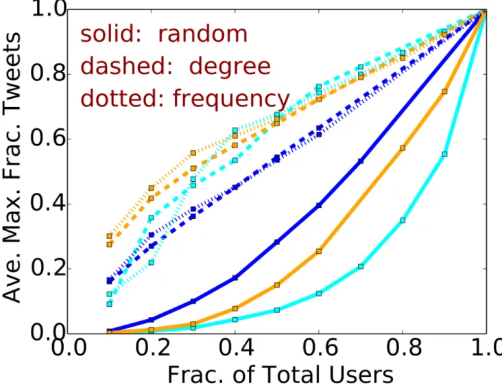
vappearing in the maximum cascade for a (country,Δ) pair; this is a high-degree heuristic. The second (dynamical) heuristic simply chooses theknodes with the greatest frequency of oc-currence in a cascade. In both heuristics,k=pNc, wherepis the probability of selecting a node (cf. previous subsection) andNcis the number of nodes in an original cascade, making it con-sistent with the earlier analysis. We compare these with a random selection of users with prob-abilityp.Fig 5shows the (normalized) maximum size of a cascade for each of the above heuristics (labeled“degree”,“frequency”and“random”, respectively), averaged over 50 trials.
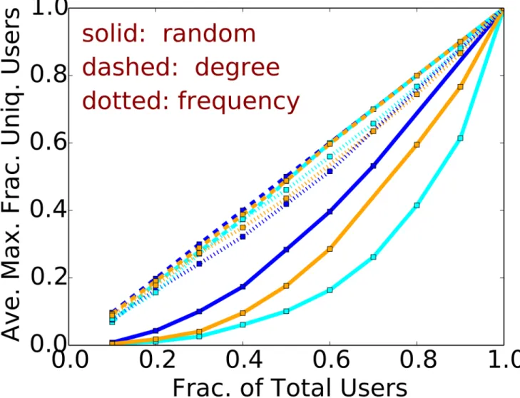
Fig 6shows the corresponding normalized maximum number of unique users in the cascades.
Fig 3. Node and shell removal heuristics for CSSP (Brazil).Here, we see the largest remaining sub-cascade size in terms of numbers of tweets (normalized by the original size) as a function of numbers of remaining nodes in the cascade graph (normalized by the original number of nodes). This cascade occurred in June 2013, and its original size is 15,791 tweets.
The normalization constant in each plot is the empirically determined maximum cascade size and maximum number of users, respectively. We find that the high degree heuristic generally produces the largest cascades in terms of tweets and users. For ordinate values in the range 0.2 to 0.4, the maximum sizes for the high degree heuristic are 2× to 10× those of the random ristic. These data indicate that large cascades are tenuous; e.g., even with the high degree heu-ristic, 80% of the original users are required to produce a cascade that is 80% of the maximum measured size. Thus, it is not the case that a few users drive cascade formation. However, for CSSP, removal of a smaller fraction (*10–20%) of users can significantly reduce cascade size.
Fig 4. Node and shell removal heuristics for CSSP (Venezuela).Here, we see the largest remaining sub-cascade size in terms of numbers of tweets (normalized by the original size) as a function of numbers of remaining nodes in the cascade graph (normalized by the original number of nodes). This cascade occurred in April 2013, and its original size is 226,179 tweets.
4.3 Illustrative Results of Tweet Contents
What types of tweets form large activity cascades that are predictive of protests? There are at least two broad classes of such tweets that we highlight here. The first kind pertains to tweets as an early reporting mechanism that then go on to form activity cascades that can serve as a pro-test recruitment or mobilization staging ground. The second kind are tweets that explicitly call for protest action by individuals.
As an example of the first kind, we discuss two tweets with a high retweet count found in our MRT cascades for Brazil. The original tweets were sent on January 27, and they are about a past event (night club fire) which led to the deaths of 231 people in Santa Maria. These tweets eventually formed part of a cascade that corresponded to an actual demonstration that took place on January 28, 2013. According to the news articles, 35,000 people marched and held a
Fig 5. Greedy heuristic for CSFP.The (normalized) maximum cascade size vs. the fraction of users selected for some of the largest cascades in different countries. Data are: blue (Mexico,Δ= 1 hour); light blue (Brazil,Δ= 4 hours); and orange (Venezuela,Δ= 4 hours).
moment of silence in front of the gymnasium where the victims’bodies had been identified. This shows that tweets selected by our vocabulary and tracked for activity cascade formation may indeed correspond to actual protest events on the ground. The second kind is highlighted by a tweet calling for a protest on September 7, illustrating that further analysis of tweets origi-nating from such cascades can aid in forecasting.
4.4 Cascade Feature Utility for Forecasting
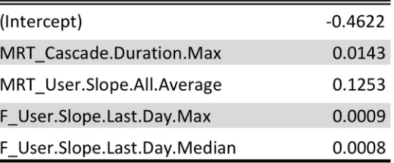
Fig 7illustrates descriptive statistics of selected features of mention and follower graph cas-cades in Brazil.Fig 8shows the variables selected by the LASSO based logistic regression model. The LASSO based model finds that the probability of an event depends upon the dura-tion and the slope of the follower and MRT graphs. These selected features are used as
Fig 6. Greedy heuristic for CSFP.The (normalized) maximum number of unique users vs. the fraction of users selected for some of the largest cascades in
different countries. Data are: blue (Mexico,Δ= 1 hour); light blue (Brazil,Δ= 4 hours); and orange (Venezuela,Δ= 4 hours).
Fig 7. Descriptive statistics of selected features (Brazil) for the MRT and F models.The names in the first column consist of the name of the structural feature (i.e., cascade size, duration or slope, which is the incremental increase in the size per day), and the statistical operations (i.e. median, average etc.).
doi:10.1371/journal.pone.0128879.g007
Fig 8. LASSO Variables.Variables selected by LASSO in the cascade model for Brazil, for a training period of November 2012 through May 2013.
explanatory variables in a generalized linear regression model [41] which confirms their signifi-cance and relevance.
4.5 Comparison Against Baseline Models
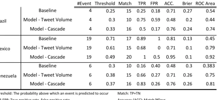
Fig 9compares the performance of the baseline model, volume-based model and the cascade model for the three countries. For each model, we report the threshold used, true positive rate (TPR), false positive rate (FPR), accuracy (ACC), brier score, and the area under the ROC curve. The results inFig 9report the threshold that results in the highest accuracy in prediction.
Note that the cascade model outperforms both the baseline model and the volume-based model. Figs10and11shows the ROC for these models. Each point in the line represents a dif-ferent threshold for the model.
Model Robustness Across Countries:Fig 9shows the performance of the cascade model for Brazil, Venezuela and Mexico. For Mexico, there are 20 matches out of 21 prediction days which results in 95% accuracy. On the other hand, the cascade model results in 76% accuracy for Venezuela and Brazil.Fig 12illustrates the ROC plots for each of the countries at various thresholds confirming Brazil and Venezuela’s performance to be worse than Mexico.
4.6 Forecasting the Unexpected: The Brazilian Spring
In a recent wave of uprisings in Brazil, known as the Brazilian spring, demonstrations were or-ganized to protest increases in bus, train, and metro ticket prices in some Brazilian cities, which quickly grew to become Brazil’s largest unrest since 1992. These events involved the
Fig 9. Performance of the predictive models.We show the performance of the three models in terms of accuracy, brier score, and area under the ROC curve. The cascades model has the best performance accross different countries.
“General Population.”We test the performance of our cascade-based prediction model by making a retrospective forecast for the events occurred in the month of June 2013 in Brazil. In the training period (November 01, 2012 to May 30, 2013), there were 131 days (out of 212) with events that involved the general population. In the test period of June 2013, there were events almost every day (29 days out of 30). The total number of events was more than 29, since there were multiple events on some days.
For this experiment, we collected 83 million tweets between November 2012 and June 2013 from Brazil. The keyword-based filtering (select if a tweet has at least 3 keywords present) re-sulted in 890,000 tweets which were further used to generate the graphs and the cascades.
Fig 10. ROC curves for the volume-based model.We show the ROC curves for Mexico, Brazil, and Venezuela. Training period November 1, 2012 to November 9, 2013; test period November 10, 2013 to November 30, 2013.
The graph-based features were extracted for each of the cascade-based models.Fig 13 dis-plays the performance of the cascade model for Brazil in June 2013. The model results in an area of 0.86, showing good performance. However, ROC does well when the number of events is very high. Therefore, we also plot the probabilities obtained from the regression model for the test period. Note that the peaks correspond to the days when the events become nation-wide and violent.Fig 14highlights the sudden surge in the structural features of the cascades. The cascade model results in 25 matches out of 26 alerts (when the best threshold is chosen as 0.6), a performance accuracy of 0.83 and TPR of 0.86.
Fig 11. ROC curves for the baseline model.We show the ROC curves for Mexico, Brazil, and Venezuela. Training period November 1, 2012 to November 9, 2013; test period November 10, 2013 to November 30, 2013.
Conclusions
Our main contributions include: (i) a detailed analysis of activity cascades arising from protest related tweets, (ii) use of cascade features for a predictive model for protest events, (iii) a rigor-ous formulation to explain the regimes for small and large cascades, in terms of the spectral ra-dius and the node expansion, and (iv) characterizing critical sets for cascades, by means of the CSSP and CSFP formulations.
Fig 12. ROC curves for different countries.ROC curves for Mexico, Brazil and Venezuela for the cascade model. Training period November 1, 2012 to November 9, 2013; test period November 10, 2013 to November 30, 2013.
Fig 13. ROC curve for Brazil.ROC curve for different models for Brazil, for a training period of Nov 2012 through May 2013 and testing period of June 1-30, 2013.
Our results suggest that, despite their simplified notion, activity cascades are useful in char-acterizing and predicting civil unrest events. Our rigorous characterization of the conditions for having large cascades highlights the role of the overall network structure; this corroborates with other recent work on influence cascades [8].
Supporting Information
S1 Dataset. Follower cascade features.
(XLS)
S2 Dataset. MRT cascade features.
(XLS)
S3 Dataset. Keyword counts for the volume-based model.
Fig 14. Cascade properties as predictors of protest.Cascade size, number of users, and number of cascades for Follower and MRT cascades in Brazil for the period November 2012—June 2013.
Author Contributions
Conceived and designed the experiments: AM NR AV. Performed the experiments: JC GK CK. Analyzed the data: JC GK. Contributed reagents/materials/analysis tools: AM NR AV. Wrote the paper: JC GK CK AM NR AV.
References
1. Sakaki T, Okazaki M, Matsuo Y. Earthquake Shakes Twitter Users: Real-time Event Detection by So-cial Sensors. In: WWW; 2010.
2. Sankaranarayanan J, Samet H, Teitler BE, Lieberman MD, Sperling J. TwitterStand: News in Tweets.
In: ACM GIS; 2009.
3. Huang C. Facebook and Twitter key to Arab Spring uprisings: report. In: The National; 2011.
4. Milne S. Egypt, Brazil, Turkey: without politics, protest is at the mercy of the elites. In: The Guardian; 2013.
5. González-Bailón S, Borge-Holthoefer J, Rivero A, Moreno Y. The Dynamics of Protest Recruitment
through an Online Network. Scientific Reports. 2011;1: . doi:10.1038/srep00197PMID:22355712
6. Borge-Holthoefer J, Rivero A, Moreno Y. Locating privileged spreaders on an online social network. Physical Review E. 2012;. doi:10.1103/PhysRevE.85.066123
7. Galuba W, Aberer K, Chakraborty D, Despotovic Z, Kellerer W. Outtweeting the Twitterers -Predicting Information Cascades in Microblogs. In: WOSN; 2010.
8. Bakshy E, Hofman J, Mason W, Watts D. Everyones an Influencer: Quantifying Influence on Twitter. In: WSDM; 2011.
9. Kwak H, Lee C, Park H, Moon S. What is Twitter, a Social Network or a News Media? In: WWW; 2010. 10. Sun E, Rosenn I, Marlow C, Lento T. Modeling Contagion through Facebook News Feed. In: ICWSM;
2009.
11. Adar E, Adamic L. Tracking information epidemics in blogspace. In: IEEE/WIC/ACM International Con-ference on Web Intelligence; 2005.
12. Leskovec J, Adamic L, Huberman B. The dynamics of viral marketing. ACM Trans Web. 2007;. doi:10.
1145/1232722.1232727
13. Kempe D, Kleinberg JM, Tardos É. Influential nodes in a diffusion model for social networks. In: ICALP 2005; 2005.
14. Crane R, Sornette D. Robust dynamic classes revealed by measuring the response function of a social system. PNAS. 2008;. doi:10.1073/pnas.0803685105PMID:18824681
15. Simma A, Jordan MI. Modeling Events with Cascades of Poisson Processes. In: UAI; 2010.
16. Zhou K, Song L, Zha H. Learning Social Infectivity in Sparse Low-rank Networks Using Multidimension-al Hawkes Processes. In: AISTATS; 2013.
17. Ganesh A, Massoulie L, Towsley D. The effect of network topology on the spread of epidemics. Pro-ceedings of INFOCOM. 2005;.
18. Tong H, Prakash BA, Eliassi-Rad T, Faloutsos M, Faloutsos C. Gelling, and Melting, Large Graphs by Edge Manipulation. In: CIKM; 2012.
19. Prakash BA, Chakrabarti D, Faloutsos M, Valler N, Faloutsos C. Threshold conditions for arbitrary
cas-cade models on arbitrary networks. In: ICDM; 2011.
20. Becker H, Naaman M, Gravano L. Beyond Trending Topics: Real-World Event Identification on Twitter. In: ICWSM; 2011.
21. Moat HS, Curme C, Avakian A, Kenett DY, Stanley HE, Preis T. Quantifying Wikipedia usage patterns before stock market moves. Scientific reports. 2013;3: .
22. Preis T, Moat HS, Stanley HE. Quantifying trading behavior in financial markets using Google Trends. Scientific reports. 2013;3: .
23. Morales AJ, Losada JC, Benito RM. Users structure and behavior on an online social network during a
political protest. Physica A. 2012;p. 5244–5253. doi:10.1016/j.physa.2012.05.015
24. Tremayne M. Anatomy of Protest in the Digital Era: A Network Analysis of Twitter and Occupy Wall Street. Social Movement Studies: Journal of Social, Cultural and Political Protest. 2013;p. 110–126.
25. Yang J, Leskovec J. Patterns of Temporal Variation in Online Media. In: WSDM; 2011.
27. Hsieh CC, Moghbel C, Fang J, Cho J. Expert vs The Crowd: Examining Popular News Prediction Per-formance on Twitter. In: WWW. ACM; 2013.
28. Asur S, Huberman BA. Predicting the Future With Social Media. In: WI-IAT; 2010.
29. Iyengar A, Finin T, Joshi A. Content-based prediction of temporal boundaries for events in Twitter. In: IEEE Int. Conf. on Social Computing. IEEE; 2011.
30. Wang X, Gerber MS, Brown DE. Automatic Crime Prediction using Events Extracted from Twitter Posts. In: SBP; 2012.
31. Lagi M, Bertand KZ, Bar-Yam Y. The Food Crises and Political Instability in North Africa and the Middle East; 2011. ArXiv:1108.2455v1: 15 pages. Available from:http://arxiv.org/pdf/1108.2455v1.pdf.
32. Braha D. Global Civil Unrest: Contagion, Self-Organization, and Prediction. PLoS One. 2012;. doi:10.
1371/journal.pone.0048596PMID:23119067
33. Radinsky K, Horvitz E. Mining the Web to Predict Future Events. In: WSDM; 2013.
34. Weber I, Garimella VRK, Batayneh A. Secular vs. Islamist Polarization in Egypt on Twitter. In: ASO-NAM; 2013.
35. Bell S, Cingranelli D, Murdie A, Caglayan A. Coercion, capacity, and coordination: Predictors of political
violence. Conflict Management and Peace Science. 2013;. doi:10.1177/0738894213484032
36. Sandra González-Bailón JBH, Moreno Y. Broadcasters and Hidden Influentials in Online Protest Diffu-sion. American Behavioral Scientist. 2013;p. 943–965.
37. Garey M, Johnson D. Computers and Intractibility; 1979.
38. Chung F, Lu L. Connected Components in Random Graphs with Given Expected Degree Sequences.
Annals of Combinatorics. 2002; 6:125–145. doi:10.1007/PL00012580
39. Saha S, Adiga A, Vullikanti AKS. Equilibria in Epidemic Containment Games. In: The 28th AAAI Confer-ence on Artificial IntelligConfer-ence (AAAI); 2014.
40. Tibshirani R. Regression shrinkage and selection via the lasso: a retrospective. Journal of the Royal Statistical Society: Series B (Statistical Methodology). 2011; 73(3):273–282. Available from:http://dx. doi.org/10.1111/j.1467-9868.2011.00771.x. doi:10.1111/j.1467-9868.2011.00771.x