http://dx.doi.org/10.20852/ntmsci.2016217826
Sensitivity of Schur stability of systems of linear
difference equations with periodic coefficients
Ahmet Duman1, G¨ulnur C¸ elik Kızılkan1and Kemal Aydın2
1Department of Mathematics and Computer Science, Necmettin Erbakan University, Konya, Turkey 2Department of Mathematics, Selcuk University, Konya, Turkey
Received: 12 November 2015, Revised: 3 March 2016, Accepted: 4 March 2016 Published online: 18 April 2016.
Abstract: In this study, the sensitivity of Schur stability of systems of linear difference equations with periodic coefficients has been examined. The modified continuity theorems based on the parametersω1andω2have been given for Schur stability of linear difference equations with periodic coefficients. Also, new results have been obtained for sensitivity ofω∗−Schur stability based on the parameters
ω1andω2. All the results have been applied to linear difference equations with periodic coefficients with orderk.kD−ball regions of Schur stability andω∗−Schur stability have been determined. In addition, the results related tokD−ball regions have been given.
Keywords: difference equation systems, monodromy matrix, periodic coefficients, Schur stability parameters, practical Schur stability, sensitivity.
1 Introduction
LetA(n)is aT−periodic matrix with N×N dimension andx(n)is an N dimensional vector. Consider the following difference equation system:
x(n+1) =A(n)x(n),x(0) =x0, n∈Z. (1)
LettingT=1, the coefficientA(n)reduces to the constant coefficientA(n+1) =A(n) =A. In the present case, the Cauchy problem (1) becomes a Cauchy problem with constant coefficients as follows,
x(n+1) =Ax(n),x(0) =x0,n∈Z. (2)
The stability property of the Cauchy problem (2) with constant coefficients is well-known in the literature (see, for example, [1,2,3]). According to the spectral criterion, if all eigenvalues of the matrix A belong to the unit disc, i.e. |λi(A)|<1 (i=1,2, . . . ,N), then the matrix A is called to be an discrete−asymptotic stable matrix. Therefore, the
system (2) is also called asdiscrete−asymptotic stable system(see, for example, [1,2,3,4]).
However, in the planeC, define the regionCS={z∈C:|z|<1}. Ifσ(A)⊂CSthenA∈RN×N is said to beSchur stable matrix, whereσ(A)is the spectrum ofA([5]).
It is well-known in the literature that eigenvalue problem of non-self-adjoint matrices is an ill-possed problem (see, for example, [4,6]). For this reason, the parameters revealing the quality of the stability obtained by avoiding calculation of eigenvalues are preferred to investigate stability.
Schur stability parameterω(A)for the systems (2) is defined as:
ω(A) =||H||; H= ∞
∑
k=0
(A∗)kAk, H=H∗>0, A∗HA−H+I=0,
whereIis unit matrix,A∗is adjoint of the matrixA,||A||=max∥x∥=1∥Ax∥is the spectral norm of the matrixA, the norm ∥x∥ is Euclidean norm for the vector x= (x1,x2, ...,xN)T. Linear difference system (2) is Schur stable if and only if
ω(A)<∞holds [7]. Let 1<ω∗∈Rbe the practical Schur stability parameter of the system (1). Then the matrixAis
called as practically Schur stable (ω∗−Schur stable) ifω(A)≤ω∗holds. Otherwise the matrixAis called asω∗−Schur
unstable matrix (see, for example, [1,4,7]). We should note here that the ω∗ practical Schur stability parameter
determined by the user according to their physical problem.
We shall be focused on the sensitivity of Schur stability of the linear difference equation system with periodic coefficients. The solutionX(n)of the equation
X(n+1) =A(n)X(n),X(0) =I,n=0,1,2, ...
is called a fundamental matrix of (1), whereA(n) =A(n+T)and theX(T)is called a monodromy matrix defined as
X(T) =
T−1
∏
j=0
A(j) =A(T−1)A(T−2)...A(1)A(0)
(see, for example, [1,2,8]).
Similar to determinating the Schur stability of the coefficient matrixA of the systems with constant coefficients given above, spectral criterion for Schur stability of monodromy matrixX(T)of the system (1) is as follow.
If|λi(X(T))|<1(i=1,2, . . . ,N) (σ(X(T))⊂CS)then the monodromy matrixX(T)is Schur stable. Schur stability of
the monodromy matrixX(T)implies that the linear difference Cauchy problem with periodic coefficients (1) is Schur stable (see, for example, [2,8]). Schur stability parameters for the systems with periodic coefficients consist of two different parameters. First of the parameters isω1(A,T)which is given by
ω1(A,T) =||F||;F=
∞
∑
k=0
(X∗(T))k(X(T))k,F=F∗>0.
If theLyapunov difference matrix equation(LDME)X∗(T)FX(T)−F+I=0 has a positive defined symmetric solution
F=F∗>0 then the linear difference system with periodic coefficients (1) is Schur stable (ω1(A,T)<∞), otherwise the system is not Schur stable.
Second of the parametersisω2(A,T)is given by
ω2(A,T) =||Φ||;Φ=
∞
∑
k=0
HereΦ is given as follows,
Φ= ∞
∑
k=0
(X∗(T))kC(X(T))k,C=
T−1
∑
i=0
X∗(i)X(i),X∗(T)ΦX(T)−Φ+C=0.
The linear difference system with periodic coefficients (1) is Schur stable if and only if the LDMEX∗(T)ΦX(T)−Φ+
C=0 has a positive defined symmetric solutionΦ =Φ∗>0 [8]. Furthermore, the system (1) is called as practically Schur stable by providing thatωi(A,T)≤ω∗, i=1,2. Otherwise, the system (1) is called asω∗−Schur unstable [9].
2 Sensitivity of Schur stability of systems of linear difference equations
It is important to predict the behaviour of solutions of a problem and to know under which conditions similar properties are protected under perturbations to avoid the problem causes any chaos. The question ”how much perturbation is ignorable for preserving the characteristic properties?” is known as the sensitivity problem.
In this section, we give some results in the literature on the sensitivity of the Schur stability of the systems with constant and periodic coefficients.
2.1 Symbols
Before introducing our theorems, we need to give the following definitions
α=T∑−1
i=0
∥X(i)∥2, Q(n,s) =n∏−1
j=s
A(j), Ψ(n,s) =n∏−1
j=s
B(j), γ= (T−1)max
1≤k≤T∥Q(T,k)∥,
β= max
1≤k≤T∥Q(T,k)∥ (
1+ (T−1) max
1≤k≤T−1∥Q(k,0)∥
)
,
µ= max
1≤k≤T∥Q(T,k)∥ × max
0≤k≤T−2∥A(j)∥; 0≤maxk≤T−2∥A(j)∥ ≤1
(
max
0≤k≤T−2∥A(j)∥
)T−2 ; max
0≤k≤T−2∥A(j)∥>1 ,
∆=Y(T)−X(T), ∆1=
√
∥X(T)∥2+ω 1
1(A,T)− ∥X(T)∥, ∆2=
√
∥X(T)∥2+ω α
2(A,T)− ∥X(T)∥,
∆3= max
0≤k≤T−1∥B(k)∥
[
β+γ max
1≤k≤T−1∥Ψ(T,k)∥+µ1max≤k≤T∥Q(T,k)∥ T−1
∑
k=2
k−1 ∑
l=1
( k!
l!(k−l)!
(
max
0≤j≤k−1∥B(j)∥
)l)]
,
∆4= max
1≤j,k≤T∥Q(j,k)∥ (
1+(T−1) max
1≤k≤T−1∥X(k)∥ )
1−(T−1) max
1≤j,k≤T∥Q(j,k)∥0≤maxk≤T−1∥B(k)∥
max
0≤k≤T−1∥B(k)∥, ∆5=
√
∥X(T)∥2+ 1
ω2(A,T)− ∥X(T)∥,
∆1∗=√∥X(T)∥2+ω∗−ω1(A,T) ω∗ω
1(A,T) − ∥X(T)∥, ∆
∗
2=
√
∥X(T)∥2+ω∗−ω2(A,T) ω∗ω
2.2 Sensitivity of Schur stability of systems with constant coefficients
Let us give the following result which shows us how much perturbation is permissible for the autonomous difference equation system
y(n+1) = (A+B)y(n), n∈Z, (3)
whereBis a constant matrix withN×Ndimensional. The system (3) is perturbated system of (2).
Theorem 1.Suppose that A is a Schur stable matrix, that isω(A)<∞. If the matrix B satisfies∥B∥<√∥A∥2+ω(A)1 −∥A∥, then A+B is Schur stable. Moreover, the inequality
|ω(A+B)−ω(A)| ≤ (2∥A∥+∥B∥)∥B∥ω 2(A)
1−(2∥A∥+∥B∥)∥B∥ω(A),
holds ([10]; Theorem 4).
2.3 Sensitivity of Schur stability of systems with periodic coefficients
In the literature, some results are given under which conditions the perturbated system
y(n+1) = (A(n) +B(n))y(n), B(n+T) =B(n), n∈Z, (4)
preserves the Schur stability when the system (1) is Schur stable (see, for example, [11,12]). Some of these results give explicit conditions for bounds of the Schur stability parameters of the system (1) and its perturbated system (4), while some of the results provide bounds for the difference between the monodromy matricesY(T)andX(T)of the systems (1) and (4), respectively. Such theorems in general known as the continuity theorems.
In this section, we give some continuity theorems of the system with periodic coefficients.
Theorem 2.Let the system (1) is Schur stable, X(T)and Y(T)be the monodromy matrices of (1) and (4), respectively.If
the matrix B(n)satisfies
∥Y(T)−X(T)∥<
√
∥X(T)∥2+ 1 ω1(A,T)
− ∥X(T)∥,
then the system (4) is Schur stable ([11]; Theorem 2). Moreover, the inequality
eF−F≤
(
2∥X(T)∥ ∥Y(T)−X(T)∥+∥Y(T)−X(T)∥2)∥F∥
1−(2∥X(T)∥ ∥Y(T)−X(T)∥+∥Y(T)−X(T)∥2)∥F∥
ω1(A,T)
holds, whereFe= ∑∞
k=0
(Y∗(T))k(Y(T))k([11]; Theorem 3).
Theorem 3. Let X(T) and Y(T) be the monodromy matrices of the systems (1) and (4), respectively, then
∥Y(T)−X(T)∥ ≤∆3. Moreover, if (1) is Schur stable, then for the perturbation matrix B(n)satisfying ∆3<∆1, the
system (4) is Schur stable too ([13]; Theorem 3).
Theorem 4. Let X(T) and Y(T) be the monodromy matrices of the systems (1) and (4), respectively, and
(T −1) max
system,then (4) is Schur stable too provided that B(n)satisfies
∥B(n)∥< ∆1 max
1≤j,k≤T∥Q(j,k)∥ [
1+ (T−1)
(
max
1≤k≤T−1∥X(k)∥+∆1
)]
([13]; Theorem 4).
Theorem 5. Let the system (1) be Schur stable, and B(n) be a perturbation matrix satisfying each of the following
conditions.
(i) ∆3<∆2,
(ii) ∥B(n)∥< ∆2
max
1≤j,k≤T∥Q(j,k)∥ [
1+(T−1) (
max
1≤k≤T−1∥X(k)∥+∆2 )],
then the perturbated system (4) is Schur stable too ([13]; Theorem 5).
3 Main results
3.1 Sensitivity of linear difference equations systems with periodic coefficients
In this part, we give upper bounds for difference between Schur stability parameters of the systems (1) and (4), upper bounds for Schur stability parameters of the system (4). In addition to the following lemma give a symmetric positive difinite matrixC=C∗>0 which satisfies LDME for Schur stable matrixX(T)( orY(T)).
Lemma 1.Let the systems (1) and (4) be Schur stable.
(i) LDME of the system (1) is satisfied by symmetric positive matrix
C=C2+∆∗FXe (T) +X∗(T)Fe∆+∆∗Fe∆,
where the positive definite matrixF is solution of LDME of the system (e 4) for any a matrix C2=C2∗>0,
(ii) For any matrix C1=C∗1>0, in correspondence to the solution F=F∗>0which satisfies LDME of system (1),
the symmetric positive definite matrix satisfing LDME of the system (4) is
C=C1+∆∗F∆−∆∗FY(T)−Y∗(T)F∆.
Proof. (i) Since the system (1) is Schur stable, that is monodromy matrixX(T)is Schur stable, there is a positive definite solution of LDME
X∗(T)FX(T)−F+C1=0;C1=C1∗>0
which isF=F∗>0 and since the system (4) is also Schur stable, there is a positive definite solution of LDME
Y∗(T)FYe (T)−Fe+C2=0;C2=C2∗>0, (5)
which isFe=Fe∗>0. Lets seek the matrixCsatisfying
forX(T)andFe=Fe∗>0 which is the solution of (5). In equation (5), if we replaceY(T)byX(T) +∆, it yields the following equation
(X(T) +∆)∗Fe(X(T) +∆)−Fe=−C2 and we have
X∗(T)FXe (T)−Fe=−(C2+∆∗FXe (T) +X∗(T)Fe∆+∆∗Fe∆
)
.
Thus we obtain LDME of the system (1) satisfied by symmetric positive matrix
C=C2+∆∗FXe (T) +X∗(T)Fe∆+∆∗Fe∆.
(ii) The proof is similar to Lemma1(i) proof.
Example 1. Let A(n) =
(
0.99 0 0 (−21)n
)
for the system (1). Perturbate the system (1) with
B(n) =
(
0.0099 0 0 (−1)n0.0099
)
.
(i) According to Lemma1(i)C=C∗=
(
197.03 0 0 1.26689
)
is obtained which satisfies LDME of the system (1) for
the symmetric positive definite matrixC2=
(
1.9998 0 0 1.26
)
which satisfies LDME of the system (4),
(ii) According to Lemma1(ii),C=C∗=
(
0.02009749 0 0 1.2432
)
is obtained which satisfies LDME of the system (4)
for the symmetric positive definite matrixC1=
(
1.9801 0 0 1.25
)
which satisfies LDME of the system (1).
Now lets re-express Continuity Theorem given with Theorem2for the parameterω1(A,T)by considering Theorem3and
4.
Theorem 6.Let the system (1) be Schur stable, ( i.e.ω1(A,T)<∞). For the matrix B(n)that satisfies the inequality
∥B(n)∥< ∆1 max
1≤j,k≤T∥Q(j,k)∥ [
1+ (T−1)
(
max
1≤k≤T−1∥X(k)∥+∆1
)]
following inequalities hold
ω1(A+B,T)≤1−(2∥X(Tω)∥1+(A∆,4T))∆4ω1(A,T);
eF−F
≤ (2∥X(T)∥+∆4)∆4ω1(A,T)2
1−(2∥X(T)∥+∆4)∆4ω1(A,T).
Proof.The proof is similar to that of Theorem2and is obtained by replacing∥Y(T)−X(T)∥by∆4, so we omit the details.
Remark 1.In Theorem2, the upper bounds in obtained inequalities depend on∥Y(T)−X(T)∥, thereby depends on the uncalculated matrixY(T)of perturbed system. On the other hand, in Theorem6, these upper bounds totally depend on the perturbation matrixB(n)which guarantees the Schur stability of system (1). Therefore, the calculation of upper bounds in inequalities in Theorem6is more adventageous than that in Theorem2. Furthermore, for perturbation matrixB(n)that satisfies the boundary condition in the inequality∥Y(T)−X(T)∥<∆1in Theorem2, if one uses∆1without calculating the matrixY(T)in inequalities in Theorem6, then the following equation is obtained:
(
2∆1∥X(T)∥+∆12
)
In that case, inequalities in Theorem2would be meaningless.
Remark 2. For the perturbation matrixB(n)which satisfies the condition ∆3<∆1, the inequalities in Theorem6are
also valid for∆3.
Example 2.Let us consider the equation
x(n+1) =
(
0.99 0 0 (−21)n
) x(n).
The monodromy matrix of the system is
X(2) =
(
0.9801 0 0 −0.25
)
,
and its condition number isω1(A,2) =25.3781. Perturbation boundary whose Schur stability is guaranteed by Theorem
6of given Schur stable system is∥B(n)∥<0.000990101. However, an obvious boundary like this cannot be given using Theorem2. For the perturbation matrix
B(n) =
(
0.0099 0 0 (−1)n0.0099
)
, max
0≤k≤1∥B(k)∥=0.0099,
ω1(A+B,2) =2500.38 and|ω1(A+B,2)−ω1(A,2)|=2475.0019. Using Theorem6without calculating matrixY(T) and only depending on the arguments of the system and matrixB(n), right hand side of the first inequality is calculated as 244924.38 and right hand side of the second inequality is calculated as 244899.002378. In contrast to that, to calculate the right hand sides of inequalities in Theorem2, the matrixY(T)must be calculated first.
Expression of Theorem6forT=1.
Corollary 1.Suppose that the system (1)(the system (2)) is Schur stable. If the matrix B satisfies∥B∥<√∥A∥2+ 1
ω(A)−
∥A∥,then the system (4)(the system (3)) is Schur stable too. Moreover, the inequalities
ω(A+B)≤1−(2∥A∥+ω∥(A)B∥)∥B∥ω(A); eF−F
≤1(−2∥(2A∥∥A+∥∥+B∥∥B)∥∥)B∥∥Bω∥2ω(A)(A)
hold.
Proof. For systems with periodic coefficients, in case of T = 1, we have A(n) =A, B(n) = B, X(T)|T=1 =A, ω1(A,T)|T=1=ω(A), ∆1|T=1=
√
∥A∥2+ω(A)1 − ∥A∥ and ∆4|T=1=∥B∥. Here, for convenience, we assume that
max
i≤k≤j,j<i{.}=0 and j
∑
k=i,j<i
(.) =0. Thus the proof is completed.
It is clear that, Corollary1is completely the same as Theorem1. This shows us that Theorem6is compatible with the results in literature. Now let us give a variant, in terms of the parameterω2of Theorem6.
Theorem 7.Let the system (1) be Schur stable, ( i.e.ω2(A,T)<∞). For a perturbation matrix B(n)which satisfies the
inequality
∥B(n)∥< ∆5 max
1≤j,k≤T∥Q(j,k)∥ [
1+ (T−1)
(
max
1≤k≤T−1∥X(k)∥+∆5
the system (4) is Schur stable. Moreover, the following inequalities hold
ω2(A+B,T)≤1−(2∥X(T)ω∥2+(A∆,T)
4)∆4ω2(A,T);
eF−F
≤ (2∥X(T)∥+∆4)∆4ω2(A,T)2
1−(2∥X(T)∥+∆4)∆4ω2(A,T).
Proof.The proof is easily obtained by considering the inequalitiesω1(A,T)≤ω2(A,T), 1/ω1(A,T)≤α/ω2(A,T)and using Theorem6.
Remark 3. For perturbation matrixB(n)which satisfies the condition∆3<∆5, inequalities given in Theorem7is also valid for∆3. ForT =1, the statement of Theorem7is the same as the statement of Corollary1. Indeed, in case ofT =1, we have
A(n) =A, B(n) =B, X(T)|T=1=A, ω2(A,T)|T=1=ω(A),
∆5
max
1≤j,k≤T∥Q(j,k)∥ [
1+ (T−1)
(
max
1≤k≤T−1∥X(k)∥+∆5
)] T=1 = √
∥A∥2+ 1
ω(A)− ∥A∥,
ω2(A,T)
1−(2∥X(T)∥+∆4)∆4ω2(A,T)
T=1
= ω(A)
1−(2∥A∥+∥B∥)∥B∥ω(A),
(2∥X(T)∥+∆4)∆4ω2(A,T)2 1−(2∥X(T)∥+∆4)∆4ω2(A,T)
T=1
= (2∥A∥+∥B∥)∥B∥ω
2(A)
1−(2∥A∥+∥B∥)∥B∥ω(A).
Thus Corollary1is obtained.
Theorem7, like Theorem6, is also compatible with the results in literature.
Example 3.Let’s consider the systemx(n+1) =Ai(n)x(n),(i=1,2)and
A1(n) =
((−1)n
4 0.2 0.4 (−51)n
)
,A2(n) =
(
0.99 32 0 (−21)n
)
.
For these systems we obtainω1(A1,2) =1.002,ω1(A2,2) =107.377 and ω2(A1,2) =1.30124,ω2(A2,2) =213.775. These systems are Schur stable. Let’s apply a perturbation to the system which has coefficient matrixA1(n)using following matrices
B11(n) =
(
(−1)n0.2 0 0 0.2
)
,B21(n) =
(
(−1)n0.2 0 0.1 0
)
.
and apply another perturbaton to the system which has coefficient matrixA2(n)using following matrices
B1 2(n) =
(
0.0001 0 0 (−1)n0.0001
)
,B2 2(n) =
(
0 0.0001 0(−1)n0.0001
)
.
According to these matrices, following results are obtained.
ω1(A1+B11,2) =1.05289,ω1(A1+B21,2) =1.03229, ω1(A2+B12,2) =108.446,ω1(A2+B22,2) =107.377, ω2(A1+B11,2) =1.5941, ω2(A1+B21,2) =1.56593, ω2(A2+B12,2) =215.913,ω2(A2+B22,2) =213.773.
(1) M=|ω1(A+B,T)−ω1(A,T)| (2) N=|ω2(A+B,T)−ω2(A,T)| (3) Mi= (2∥X(T)∥+∆i)∆iω1(A,T)
2
1−(2∥X(T)∥+∆i)∆iω1(A,T),(i=3,4)
(4) Ni= (2∥X(T)∥+∆i)∆iω2(A,T)
2
1−(2∥X(T)∥+∆i)∆iω2(A,T),(i=3,4)
(5) Pi=1−(2∥X(T)ω1∥+(A∆,Ti))∆iω1(A,T),(i=3,4)
(6) Ti=1−(2∥X(T)ω2∥(A+∆,Ti))∆
iω2(A,T),(i=3,4).
Now considering the given data, let’s comment on Theorems6and7using the Table 1 and Table 2.
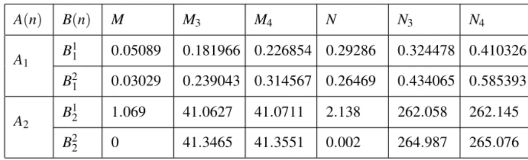
A(n) B(n) M M3 M4 N N3 N4
A1
B11 0.05089 0.181966 0.226854 0.29286 0.324478 0.410326
B21 0.03029 0.239043 0.314567 0.26469 0.434065 0.585393
A2
B12 1.069 41.0627 41.0711 2.138 262.058 262.145
B22 0 41.3465 41.3551 0.002 264.987 265.076
Table 1:This table illustrates the upper bounds ofMandNin Theorem6and Theorem7.
As seen in Table 1,MiandNi(i=3,4)which are the upper bounds of differences of condition numbers of perturbed and
non perturbed systems given in Theorem6and Theorem7, are affected by perturbation and therefore when perturbation is changed, healthy information can be obtained about the change of difference between Schur stability parameters of system (1) and system (4). As seen in the table, the upper boundsMiandNi (i=3,4)of the differencesM andNgive
closer results to occuring differences when the quality of Schur stability is stronger (i.e. the parameter value is smaller). For example, for the coefficient matrixA1(n)and the perturbation matrixB12(n), the occuring differences areM=0.03029 andN=0.26469 which has upper boundsM3=0.239043,M4=0.314567 andN3=0.434065,N4=0.585393 which are closer to occuring differences. However, for the coefficient matrixA2(n), which has lower quality of Schur stability with compare toA1(n), the upper bounds are much greater than differences occured.
A(n) B(n) ω1(A+B,T) P3 P4 ω2(A+B,T) T3 T4
A1
B11 1.05289 1.18397 1.22885 1.5941 1.62572 1.71157
B21 1.03229 1.24104 1.31657 1.56593 1.73531 1.88663
A2
B1
2 108.446 148.44 148.448 215.913 475.833 475.92
B2
2 107.377 148.723 148.732 213.773 478.762 478.851
Table 2:This table illustrates the upper bounds ofω1(A+B,T)andω2(A+B,T)in Theorem6and Theorem7.
As seen in Table 2,PiandTi(i=3,4)which are the upper bounds of parameters of Schur stability of the perturbation
system given in Theorem6 and Theorem 7, are affected by the perturbation, so when perturbation changes, healthy information can be obtained about Schur stability parameters of the system (4). As seen in the table,PiandTi(i=3,4),
values areω1(A1+B11,2) =1.05289 andω2(A1+B11,2) =1.5941.The upper boundsP3=1.18397,P4=1.22885 and
T3=1.62572,T4=1.71157 of these values are closer to these values. However, for the coefficient matrixA2(n)which has lower quality of Schur stability, the upper bounds are much greater than the values occured.
3.2
ω
∗−
Schur stability of linear difference equation systems with periodic coefficients
In this section, some results on the sensitivity of theω∗−Schur stability are investigated.
Theorem 8.Let the system (1) be ω∗−Schur stable ( i.e.ω
i(A,T)≤ω∗, i=1,2), and B(n)be a perturbation matrix satisfying each of the following conditions:
(i) ∆3≤∆i∗; i=1,2,
(ii) ∥B(n)∥ ≤ ∆i∗
max
1≤j,k≤T∥Q(j,k)∥ [
1+(T−1) (
max
1≤k≤T−1∥X(k)∥+∆
∗
i
)]; i=1,2,
then the perturbated system (4) isω∗−Schur stable too.
Proof. (i) Since ωω∗∗−ωωi(A,T)
i(A,T) <
1
ωi(A,T) ≤ α
ωi(A,T), the inequality∆3≤∆
∗
i <∆i(i=1,2)is hold. Thus the perturbated
system (4) is Schur stable according to Theorem3and5. Therefore if the inequality
∆3≤∆i∗= √
∥X(T)∥2+ω∗−ωi(A,T) ω∗ω
i(A,T)
− ∥X(T)∥,i=1,2
is solved forω∗, the inequality
ωi(A,T)
1−(2∥X(T)∥+∆3)∆3ωi(A,T)
≤ω∗,i=1,2
is obtained. Thus the system (4) isω∗−Schur stable from Theorem6and7and Remark 1. and 2.
(ii) If the inequality∥B(n)∥ ≤ ∆i∗
max
1≤j,k≤T∥Q(j,k)∥ [
1+(T−1) (
max
1≤k≤T−1∥X(k)∥+∆
∗
i
)]is solved for∆∗
i,i=1,2, the inequality
∆4≤∆i∗,i=1,2
is obtained. Sinceωω∗∗−ωωi(Ai(A,T,T))<ω 1
i(A,T)≤
α
ωi(A,T), the inequality∆4≤∆i∗<∆i(i=1,2)is hold. Thus the perturbated
system (4) is Schur stable. Therefore if the inequality
∆4≤∆i∗= √
∥X(T)∥2+ω∗−ωi(A,T) ω∗ω
i(A,T)
− ∥X(T)∥,i=1,2
is solved forω∗, the inequality
ωi(A,T)
1−(2∥X(T)∥+∆4)∆4ωi(A,T)
≤ω∗,i=1,2
is obtained. Thus the system (4) isω∗−Schur stable from Theorem6and7.
Example 4.For the system (1) letA(n) =
(
0.9 0.1 0 (−101)n
)
andω∗=10. Sinceω
0.0647958,∥B(n)∥ ≤0.0269713 and∥B(n)∥ ≤0.0666285,∥B(n)∥ ≤0.0266247 which are obtained using Theorem8 (i) and Theorem 8 (ii), respectively, the system (4) is ω∗−Schur stable. For example, let the perturbation matrix be
B(n) =
(
0.026 0 0 (−1)n0.026
)
, then∥B(n)∥=0.026. Indeed for the system (4),A(n) +B(n) =
(
0.926 0.1 0 (−1)n0.126
)
and it can be seen thatω1(A+B,2) =3.81806≤ω∗andω2(A+B,2) =7.10177≤ω∗.
3.3 Application of the results on the sensitivity of linear difference equations with order k
Consider the following linear difference equations with orderk
x(n+1)−a0(n)x(n)−. . .−ak−1(n)x(n−k+1) =0 (6)
for n≥0 andai(n) =ai(n+T),i=0,1,2, ...,k−1,T >0. By takingx(n−k+1) =y1(n),x(n−k+2) =y2(n),... ,
x(n) =yk(n)the equation (6) can be written as
y(n+1) =C(n)y(n),n≥0 andC(n+T) =C(n) (7)
in matrix-vector form, where the matrixC(n)is companion matrix as follows
C(n) =
0 1 0 · · · 0 0 0 1 · · · 0
..
. ... ... . .. ... 0 0 0 · · · 1
ak−1(n)ak−2(n)ak−3(n)· · · a0(n)
.
Thus, the results on the sensitivity of Schur stability which are given for the system (1) can easily be used for the sensitivity of Schur stability of the linear difference equations with orderk(6).
Consider the perturbation of the equation (6), and so, of the system (7)
z(n+1) = (C(n) +D(n))z(n),n≥0,D(n+T) =D(n), (8)
where
D(n) =
0 0 0 · · · 0 0 0 0 · · · 0
..
. ... ... . .. ... 0 0 0 · · · 0
dk−1(n)dk−2(n)dk−3(n)· · · d0(n)
,
di(n) =di(n+T),T≥0,i=0,1,2, ...,k−1.
The set Bδ called as the kD−ball, i.e. the k−dimensional ball [14], and defined as
Bδ ={x= (x1,x2, . . . ,xk)| ∥x(n)∥<δ}. Let
•d(n) = (dk−1(n),dk−2(n), . . . ,d1(n),d0(n)), •δi= ∆i
max
1≤j,k≤T∥Q(j,k)∥ [
1+(T−1) (
max
1≤k≤T−1∥X(k)∥+∆i
•δ∗
i =
∆∗
i
max
1≤j,k≤T∥Q(j,k)∥ [
1+(T−1) (
max
1≤k≤T−1∥X(k)∥+∆
∗
i
)],i=1,2.
For the system (7), the variant of Theorem4is as follows.
Theorem 9.Let the system (7) be Schur stable. If the k−tuple d(n)∈Bδi (i=1,2), then the perturbed system (8) is Schur stable.
Proof.Sinced(n)∈Bδi, we obtain∥D(n)∥=∥d(n)∥<δi. Therefore, if the system (7) is Schur stable, the condition
∥D(n)∥<δi;i=1,2 in Theorems4and5guarantees the Schur stability of the perturbed system (8).
Remark 4. ThekD−ballBδ occurs as a region of Schur stability for the perturbation matrixD(n). The 1D−ballBδ is an
interval, the 2D−ballBδ is a disc, and the 3D−ballBδ is the interior of a sphere, i.e. a solid ball.
Theorem 10.Let the system (7) beω∗−Schur stable. If the k-tuple d(n)∈B
δi∗(i=1,2), then the perturbed system (8) is alsoω∗−Schur stable.
Proof.The proof is easily obtained from Theorems8(ii) and9.
Example 5.Consider the delay difference equation
x(n+1)−1
4cos(nπ)x(n) =− 1
100x(n−1),n≥0. (9)
For the companion matrixC(n), it is easy to check that ω1(C,2) =1.06833 andω2(C,2) =2.13647. Therefore, the equation (9) is Schur stable.
•δ1=0.259469,δ2=0.263176, •forω1∗=3;δ1∗
(3)=0.209221 andδ
∗
2(3)=0.0828397,
•forω∗
2=10;δ1∗(10)=0.246093 andδ
∗
2(10)=0.159556.
Consider the perturbed equation
y(n+1)−
(
1
4cos(nπ) +d0(n)
) y(n) =
(
− 1
100+d1(n)
)
y(n−1), (10)
wheren≥0 anddi(n) =di(n+2),i=0,1.
•The equation (10) for all elements of the setBδi (i=1,2)is Schur stable, •The equation (10) for all elements of the setBδ∗
i(3) (i=1,2)is 3−Schur stable,
•The equation (10) for all elements of the setBδ∗
i(10) (i=1,2)is 10−Schur stable.
Ford(n) =((−1)n+10.183,(−1)n0.183), perturbate matrix
D(n) =
(
0 0
(−1)n+10.183(−1)n0.183 )
, max
0≤k≤1∥D(k)∥=0.258801.
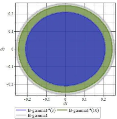
Fig. 1:Schur stability region ofBγ∗
1(3),Bγ1∗(10) andBγ1.
Fig. 2:Schur stability region ofBγ∗
Schur stability regionBδi, 3−Schur stability regionBδi∗(3) and 10−Schur stability regionBδi∗(10) of the equation (10) have
been given with Figure 1 and Figure 2. As it is clearly seen from Figure 1 and Figure 2,Bδ∗
i(3) ⊂Bδi∗(10) ⊂Bδi (i=1,2).
Theorem 11. (i) limωi→∞Bδi =∅, i=1,2,
(ii) limωi→ωi∗Bδi∗=
∅, i=1,2,
(iii) limω∗
i→∞Bδi∗ =Bδi, i=1,2.
Proof. (i) The equality limωi→∞δi = 0 holds, where limωi→∞∆i = 0, i = 1,2. Therefore,
limωi→∞{x= (x1,x2, . . . ,xn)| ∥x(n)∥<δi}=∅,
(ii) limωi→ωi∗Bδi∗=
∅for limω
i→ωi∗δ
∗
i =0,i=1,2,
(iii) limωi→ωi∗Bδi∗=
∅for limω
i→ωi∗δ
∗
i =0,i=1,2,
so the proof is obtained.
Theorem 12. (i) The sequence of set{Bδi}is increasing according toδi, i=1,2,
(ii) The sequence of set {
Bδ∗
i }
, i=1,2is bounded.
Proof. (i) Letx(n+1) =C1(n)x(n)andy(n+1) =C2(n)y(n). It is clear that if δi(C2)<δi(C1)then the inclusion
Bδi(C2)⊂Bδi(C1)holds,i=1,2,
(ii) ∅⊂Bδ∗
i ⊂Bδi for 0<δ
∗
i <
∆i
max
1≤j,k≤T∥Q(j,k)∥ [
1+(T−1) (
max
1≤k≤T−1∥X(k)∥+∆i
)],i=1,2.
Remark 5.The numerical examples have been computed by using matrix vector calculator MVC [15].
4 Conclusion
In this paper we have consider sensitivity problem for Schur stable linear difference equation system with periodic coefficients. For this problem, the upper bounds in obtained inequalities which depends on∥Y(T)−X(T)∥in continuity theorems in literature have depend on the uncalculated matrixY(T)of perturbed system. On the other hand, the similar bounds in the continuity theorems in this study totally have depend on the perturbation matrixB(n)which guarantees the Schur stability of system (1). Therefore, the calculation of upper bounds in inequalities in the continuity theorems have been more adventageous than that in continuity theorems in literature.
In addition, some new results on the sensitivity ofω∗−Schur stability have obtained. All the results have applied to
linear difference equations with periodic coefficients with orderk.kD−ball regions of Schur stability andω∗−Schur
stability have determined. Also some examples illustrating the efficiency of the theorems have given.
References
[2] Elaydi S.N.,An introduction to difference equations,New York; Springer-Verlag, (1999).
[3] Godunov S.K.,Modern aspects of linear algebra, RI: American Mathematical Society, Translation of Mathematical Monographs 175. Providence, (1998).
[4] Bulgak H., “Pseudoeigenvalues, spectral portrait of a matrix and their connections with different criteria of stability”,Error Control and Adaptivity in Scientific Computing, NATO Science Series, Series C: Mathematical and Physical Sciences, in: H. Bulgak and C. Zenger(Eds), Kluwer Academic Publishers, (1999), 536, 95-124.
[5] Voicu M. and Pastravanu O., “Generalized matrix diagonal stability and linear dynamical systems”,Linear Algebra and its Applications, (2006), 419, 299-310.
[6] Wilkinson J. H., “The algebraic eigenvalue problem”, Clarendom Pres Oxford, (1965).
[7] A.Ya. Bulgakov (H. Bulgak), “An effectively calculable parameter for the stability quality of systems of linear differential equations with constant coefficients”,Siberian Math. J.(1980), 21, 339–347.
[8] Aydın K., Bulgak H. and Demidenko G. V., “Numeric characteristics for asymptotic stability of solutions to linear difference equations with periodic coefficients”,Siberian Mathematical Journal,(2000), 41, 1005-1014.
[9] Aydın K., “Schur stable difference equations with constant coefficients”, Zonguldak Karaelmas University, Integral Geometry and Inverse Problem Workshop, May 08-09,(2004), Zonguldak.
[10] Duman A. and Aydın K., “Sensitivitiy of linear difference equation systems with constant coefficients”,Scientific Research and Essays, (2011), 6(28) 5846-5854.
[11] Aydın K., Bulgak H. and Demidenko G. V., “Continuity of numeric characteristics for asymptotic stability of solutions to linear difference equations with periodic coefficients”,Selc¸uk Journal Applied Mathematics, (2001), 2, 5-10.
[12] Aydın K., Bulgak H. and Demidenko G. V., “Asymptotic stability of solutions to perturbed linear difference equations with periodic coefficients”,Siberian Mathematical Journal,(2002), 43, 389-401.
[13] Duman A. and Aydın K., “Sensitivity of Schur stability of monodromy matrix”,Applied Mathematics and Computation, (2011), 217, 6663–6670.
[14] Roger AH., Charles RJ.,Matrix analysis,Cambridge University Press, Cambridge, (1999).