A hybrid bin scheme to solve the condensation/evaporation equation using a cubic distribution function

(1)

ACPD

11, 21631–21654, 2011

Hybrid bin scheme

T. Dinh and D. R. Durran

Title Page

Abstract Introduction

Conclusions References

Tables Figures

◭ ◮

Back Close

Full Screen / Esc

Printer-friendly Version Interactive Discussion

Discussion

P

a

per

|

Dis

cussion

P

a

per

|

Discussion

P

a

per

|

Discussio

n

P

a

per

Atmos. Chem. Phys. Discuss., 11, 21631–21654, 2011 www.atmos-chem-phys-discuss.net/11/21631/2011/ doi:10.5194/acpd-11-21631-2011

Atmospheric Chemistry and Physics Discussions

This discussion paper is/has been under review for the journal Atmospheric Chemistry and Physics (ACP). Please refer to the corresponding final paper in ACP if available.

A hybrid bin scheme to solve the

condensation/evaporation equation

using a cubic distribution function

T. Dinh and D. R. Durran

Department of Atmospheric Sciences, University of Washington, Seattle, WA 98195, USA

Received: 20 July 2011 – Accepted: 22 July 2011 – Published: 1 August 2011

Correspondence to: T. Dinh (tradinh@uw.edu)

(2)

ACPD

11, 21631–21654, 2011

Title Page

Tables Figures

◭ ◮

Back Close

Full Screen / Esc

Discussion

P

a

per

|

Dis

cussion

P

a

per

|

Discussion

P

a

per

|

Discussio

n

P

a

per

|

Abstract

A computationally efficient method is proposed to replace the piecewise linear number distribution in a hybrid bin scheme with a piecewise cubic polynomial. When the linear distribution is replaced by a cubic, the errors generated in solutions to the condensa-tion/evaporation equation are reduced by a factor of two to three. Alternatively, using 5

the cubic distribution function allows reducing the number of bins by 20_±5 % when solving the condensation/evaporation problem without sacrificing accuracy.

1 Introduction

In the microphysics context, a hybrid bin scheme is a two-moment explicit scheme designed to solve for the evolution of the size spectrum of cloud droplets and ice crys-10

tals. The particular hybrid bin scheme that is the focus of this paper is the scheme developed by Chen and Lamb (1994); hereafter referred to as the CL scheme.

The CL scheme has been implemented in meso- and synoptic-scale cloud resolving models, including the Nonhydrostatic Modeling System of the University of Wisconsin (Hashino and Tripoli, 2007) and the Goddard Cumulus Ensemble model (Przyborski, 15

2006). It has also been used in case studies of warm clouds (Kuba and Fujiyoshi, 2006; Kuba and Murakami, 2010), orographic clouds (Chen and Lamb, 1999), synoptically forced cirrostratus (Lin et al., 2005) and thin cirrus in the tropical tropopause layer (Dinh et al., 2010).

The CL scheme produces less numerical di_ffusion than one-moment bin schemes 20

and so is more accurate. Yet, because of its computational cost, it has not been im-plemented in 3-D or large-scale models. In the CL scheme, the evolution of two mo-ments (mass and number of particles) in each bin has to be evaluated, which can impose both computational and storage burdens in dynamically-coupled multidimen-sional cloud models.

(3)

ACPD

11, 21631–21654, 2011

Title Page

Tables Figures

◭ ◮

Back Close

Full Screen / Esc

Discussion

P

a

per

|

Dis

cussion

P

a

per

|

Discussion

P

a

per

|

Discussio

n

P

a

per

The CL scheme is based on a linear fit to the number distribution of microphysi-cal particles in each bin. In this paper, we show that replacing the linear distribution function by a cubic polynomial significantly reduces the error of the scheme in solving the condensation/evaporation equation. This new scheme can be used to increase accuracy, or can alternatively allow computations with fewer bins to obtain the same 5

accuracy. Such an increase in efficiency may be useful for modelers using hybrid bin schemes in cloud resolving models.

2 The hybrid bin scheme

2.1 Evolution of the number density

The evolution of the number density n=n(x,m,t) of microphysical particles (droplets

10

or crystals) is described by

∂n

∂t =−∇·(un)+ ∂

∂z(Vtn)− ∂

∂m(cn)+G (1)

wherex=(x,y,z) is the vector location in space,m is the particle mass andtis time.

The first term in Eq. (1) is advection in space by the velocity vectoru. The second term

is sedimentation of particles at the terminal fall speedVt. The third term is growth at

15

ratecby water vapor condensation onto droplets or deposition onto crystals. The last termGrepresents the aggregation process.

In a cloud resolving model, the changes inndue to the individual terms in Eq. (1) are computed separately and then summed together to give nat the next time step. Here we will concentrate on the condensation/deposition term only.

(4)

ACPD

11, 21631–21654, 2011

Title Page

Tables Figures

◭ ◮

Back Close

Full Screen / Esc

Discussion

P

a

per

|

Dis

cussion

P

a

per

|

Discussion

P

a

per

|

Discussio

n

P

a

per

|

2.2 Subgrid linear distribution

In the original CL scheme, the number densitynas a function of the mass of particles

min each bin is assumed linear and represented by

n(m)=n0+k(m−m0), (2)

and the total number and mass of particles in the bin are given as 5

N =

Zm₂

m₁

n(m)dm, _M=

Zm₂

m₁

mn(m)dm, (3)

wherem1andm2are the masses that define the bin boundaries. Equations (2) and (3)

are consistent when

n0= N

△m, k=

12_N(m₋m0)

(_△m)3 , (4)

wherem0=(m1+m2)/2,△m=m2−m1andm=M/N is the mean mass of the bin.

10

The distribution function given by Eqs. (2) and (3) may be negative in part of the bin. If that happens Chen and Lamb (1994) ensured positiveness by modifying the distribution so that it occupies only part of the bin. Ifn0+k(m1−m0)<0, they set

n(m)=

(

k_∗(m₋m_∗) if m_∗_≤m_≤m₂,

0 otherwise, (5)

where1 15

m_∗=3m₋2m2, k∗=

2_N (m₂₋m_∗)2. 1

(5)

ACPD

11, 21631–21654, 2011

Title Page

Tables Figures

◭ ◮

Back Close

Full Screen / Esc

Discussion

P

a

per

|

Dis

cussion

P

a

per

|

Discussion

P

a

per

|

Discussio

n

P

a

per

Alternatively, ifn0+k(m2−m0)<0,

n(m)=

(

k_∗(m−m_∗) if m1≤m≤m∗,

0 otherwise, (6)

where

m_∗=3m₋2m1, k∗=− 2_N (m1−m∗)2

.

2.3 Bin shift 5

LetN be the number of bins and µ1,µ2,...,µN+1 denote the grid divisions along the

mass axis. In both the original CL algorithm and our new method, the procedure to stepNj andMj forward in time for each binj involves growing the particles in the bin, shifting the bin along the mass axis and finally mapping the shifted bin onto the mass axis. The algorithm may be described by the following four steps:

10

1. The number and mass after one step of condensational/depositional growth in bin

j are calculated as ˜

Nj=Nj, ˜

Mj=Mj+Njc(mj)△t,

15

wherec(mj) is the growth rate at the mean massmj=Mj/Nj. For efficiency, all particles in the bin are assumed to grow at the rate of the mean mass of the bin.

2. The left and right boundaries of the shifted bin (m1,j andm2,j) are calculated as:

m1,j=µj+c(µj)△t, m2,j=µj+1+c(µj+1)△t,

(6)

ACPD

11, 21631–21654, 2011

Title Page

Tables Figures

◭ ◮

Back Close

Full Screen / Esc

Discussion

P

a

per

|

Dis

cussion

P

a

per

|

Discussion

P

a

per

|

Discussio

n

P

a

per

|

3. In the original CL scheme, the linear number distribution within each shifted bin is computed from ˜Nj, ˜Mj, m1,j andm2,j using Eqs. (2), (4), (5) and (6). The new procedure using the cubic distribution is discussed in the next section.

4. Find the location of the shifted bin with respect to the grid by comparing m₁_,j

andm2,j with the grid pointsµ1,µ2,...,µN+1. For each grid bin overlapped by the

5

shifted bin, integrate the distribution function of the shifted bin to find the number and mass of particles that will be accumulated in the grid bin. See Chen and Lamb (1994) for illustrations.

2.4 Subgrid cubic distribution

The slope of the linear distribution function in each bin does not depend on the distribu-10

tion in adjacent bins. As in higher-order finite volume methods, the distribution within in each bin can be more accurately estimated using information from adjacent bins. A cubic polynomial representing the number distribution in each bin can be evaluated using information from the bins immediately to the right and left (in addition to the total number and mass of the centered bin).

15

Chen and Lamb (1994) mentioned the possibility of using higher-order polynomial distributions that were continuous across bin boundaries. However, continuity at the bin boundary is not the optimal approach because, compared with other points along the mass axis within the bin, the boundaries of the bin are subject to the largest error. Indeed, the assumption that the growth rate of particles in the bin is equal to the growth 20

rate of the mean mass is least accurate at the bin boundaries. Thegrowth-of-the-mean assumption, though essential to the efficiency of the CL scheme, introduces large er-rors at the boundaries and occasionally causes the distribution to become negative there.

Hence, to derive the cubic form of the distribution for each bin, it is best to avoid 25

(7)

ACPD

11, 21631–21654, 2011

Title Page

Tables Figures

◭ ◮

Back Close

Full Screen / Esc

Discussion

P

a

per

|

Dis

cussion

P

a

per

|

Discussion

P

a

per

|

Discussio

n

P

a

per

distribution at the mean mass, denoted here byn, can be approximated by the linear form of the distribution, i.e. by evaluating Eqs. (2), (5) or (6) at the mean mass value.

Suppose that we represent the number distribution in each bin as the cubic

n(m)₌a0+a1m+a2m2+a3m3. (7)

The coefficients a0,...,a3 are to be determined by the conservation of number and

5

mass (Eq. 3) in the centered bin, and by requiring that (mL,nL) and (mR,nR) from the

left and right bins satisfy Eq. (7). Here, we need to solve a system of linear equations for four coefficientsa₀,...,a₃for each bin.

An economical solution procedure can be obtained by rewriting the number distribu-tion as a weighted sum of the four lowest order Legendre polynomials, which are 10

P0(χ)=1, (8)

P1(χ)=χ , (9)

P2(χ)=

1 2(3χ

2

−1), (10)

P3(χ)=

1 2(5χ

3

−χ), (11)

15

whereχ is an independent variable defined between₋1 and 1. A key property of the Legendre polynomials is the orthogonality condition,

Z1

−1

PjPkdχ= 2

2j+1δjk, (12)

whereδ_jk denote the Kronecker delta. If we defineχ as

χ=2(m−m0)

m2−m1

, (13)

(8)

ACPD

11, 21631–21654, 2011

Title Page

Tables Figures

◭ ◮

Back Close

Full Screen / Esc

Discussion

P

a

per

|

Dis

cussion

P

a

per

|

Discussion

P

a

per

|

Discussio

n

P

a

per

|

then asmvaries betweenm1andm2,χ varies between−1 and 1. Now the distribution

function can be written as a function ofχ:

n(χ)=b0P0(χ)+b1P1(χ)+b2P2(χ)+b3P3(χ). (14)

Based on the orthogonality property (Eq. 12), the conservation of number and mass (Eq. 3) simplifies to

5

N =△m

2

Z1

−1

(b0P0+b1P1+b2P2+b3P3)P0dχ

=b0△m,

M=△m

2

Z1

−1

(b0P0+b1P1+b2P2+b3P3)

m0P0+

△m

2 P1

dχ

=△m 2

2m0b0+△

m

3 b1

,

10

from which

b0= N

△m, (15)

b1=

6(_M−m0N)

(_△m)2 . (16)

Note that when b2=0 and b3=0, these values ofb0 and b1 are consistent with the

15

linear distribution function given by Eqs. (2) and (4).

Nextb2andb3are determined by requiring that (χ(mL),nL) and (χ(mR),nR) from the

left and right bins satisfy Eq. (14).χ(mL) andχ(mR) are Eq. (13) evaluated at the mean

(9)

ACPD

11, 21631–21654, 2011

Title Page

Tables Figures

◭ ◮

Back Close

Full Screen / Esc

Discussion

P

a

per

|

Dis

cussion

P

a

per

|

Discussion

P

a

per

|

Discussio

n

P

a

per

b0+b1χL+b2

3χ2L−1

2 +b3

5χ3L−3χL

2 =nL, (17)

b0+b1χR+b2

3χ2R−1

2 +b3

5χ3R−3χR

2 =nR, (18)

where

χL=χ(mL)=

2(mL−m0)

m2−m1

, χR=χ(mR)=

2(mR−m0)

m2−m1

.

5

Equations (17) and (18) are two linear equations of two unknowns (b2and b3), which

can be solved easily to obtainb₂andb₃.

Finally, the coefficients for the cubic distribution function in standard form are ob-tained by substituting Eqs. (8)–(11) and (13) into Eq. (14) and comparing with Eq. (7):

a0=b0−2qb1+

6q2−1

2

b2−

20q3−3qb3, (19)

10

a1=

2b1−12qb2+

60q2−3b3

△m , (20)

a2=

6b2−60qb3

(_△m)2 , (21)

a3=

20b3

(_△m)3, (22)

whereq= m0

△m.

15

(10)

ACPD

11, 21631–21654, 2011

Title Page

Tables Figures

◭ ◮

Back Close

Full Screen / Esc

Discussion

P

a

per

|

Dis

cussion

P

a

per

|

Discussion

P

a

per

|

Discussio

n

P

a

per

|

– The cubic distribution function obtains a negative minimum inside the bin, i.e., if

△=a2₂₋3a1a3≥0

and forme=−

a₂+√△

3a₃ , we havem1≤me≤m2and

n(me)=a0+a1me+a2m2e+a3m3e<0.

– The cubic distribution function is negative at the left and/or the right bin bound-5

aries, which is the case if

n(m1)=a0+a1m1+a2m2₁+a3m3₁<0,

or

n(m2)=a0+a1m2+a2m2₂+a3m3₂<0.

The only modification to the bin-shift procedure outlined in Sect. 2.3 is in Step 3, 10

which is replaced by

3. Compute the cubic distribution function using Eqs. (15)–(22), and use this dis-tribution if it is nonnegative. Otherwise use the linear disdis-tribution. The linear distribution function should also be used for the leftmost and rightmost bins.

3 Numerical tests 15

3.1 Evaporation of cloud drops

(11)

ACPD

11, 21631–21654, 2011

Title Page

Tables Figures

◭ ◮

Back Close

Full Screen / Esc

Discussion

P

a

per

|

Dis

cussion

P

a

per

|

Discussion

P

a

per

|

Discussio

n

P

a

per

3.1.1 Initial conditions

For dilute and relatively large spherical drops, the condensational growth rate can be approximated by

c=dm

dt =BSm

1/3_, ₍₂₃₎

whereS is the supersaturation ratio andB=4.7_×10−8kg2/3s−1 under standard tem-5

perature and pressure.

The initial drop spectrum is assumed to be

f(m)=N0m

m2

c exp

−_mm

c

, (24)

whereN0=2.0×10 8

m−3and mc is the mode of the distribution (wheref(m) is maxi-mum). We setm_c=3.5_×10−8kg, which is the mass of a drop whose radius is 200 µm. 10

The analytical solution to the evolution of the drop spectrum when the growth rate is given by Eq. (23) was derived by Tzivion et al. (1989). It is

n(m,t)=m−1/3_X1/2_f_X3/2_, ₍₂₅₎

whereX=m2/3−2

3BSt and f(X 3/2

) is the initial drop spectrum function evaluated at

X3/2. 15

Numerical solutions are computed for the case when drops evaporate at fixed S=

(12)

ACPD

11, 21631–21654, 2011

Title Page

Tables Figures

◭ ◮

Back Close

Full Screen / Esc

Discussion

P

a

per

|

Dis

cussion

P

a

per

|

Discussion

P

a

per

|

Discussio

n

P

a

per

|

3.1.2 Grid and time spacings

The grid points along the mass axisµ_j forj=1,2,...,N+1, whereN is the number of bins, are defined by

µj= 4 3ρπr

3

j,

rj=rminαj−1,

5

α=

_r

max

rmin

1/N

,

wherermin=1 µm andrmax=1000 µm. The grid thus spans betweenrmin andrmaxand

is more tightly spaced for small radii. The time step is_△t=1 s.

10

3.1.3 Results

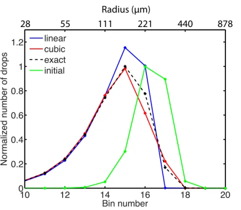
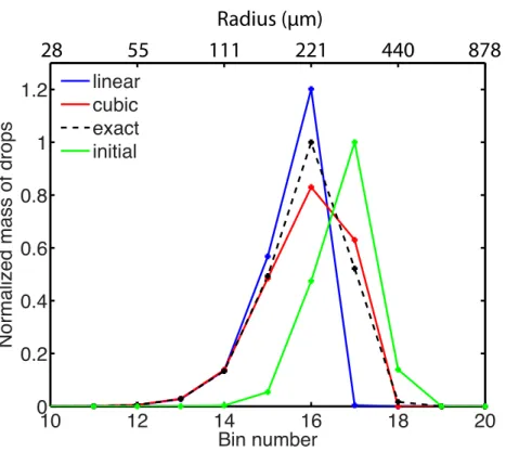
Solutions for the evaporation problem at 20-bin-resolution at 50 min are shown in Fig. 1a (number of drops per bin) and b (mass of drops per bin). The solution obtained by the cubic scheme is more accurate than that by the linear scheme. In particular, the linear scheme underestimates the number and mass of larger drops (with major 15

errors in bin 17). At this resolution, the root-mean-square errors of the linear and cubic schemes are respectively 1.22_×106m−3and 0.64_×106m−3in cloud drop number and 6.34×10−2kg m−3and 2.29×10−2kg m−3in drop mass.

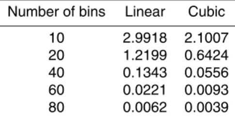
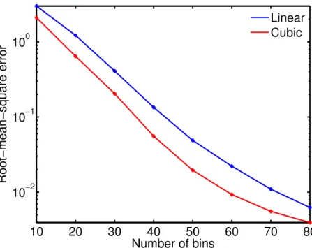
The errors of the solutions obtained by the linear and cubic schemes are given as a function of bin resolution in Table 1 and Fig. 2. At all but the coarsest resolution (10 20

(13)

ACPD

11, 21631–21654, 2011

Title Page

Tables Figures

◭ ◮

Back Close

Full Screen / Esc

Discussion

P

a

per

|

Dis

cussion

P

a

per

|

Discussion

P

a

per

|

Discussio

n

P

a

per

3.2 Depositional growth of small ice crystals

3.2.1 Initial conditions

If ice crystals are assumed spherical, the depositional growth rate can be calculated as

c=dm dt =

4πrSice

R_vT esat,iceDv′+

L_s k_a′T

_L

s

RvT−1

(26)

5

(Pruppacher and Klett, 1978, p. 448), where m and r are respectively the mass and radius of ice crystals, Rv is the gas constant for water vapor, Ls is the latent heat of

sublimation,ka′ is the modified thermal conductivity of air,Dv′ is the modified diffusivity

of water vapor in air, esat,ice is the saturation vapor pressure over plane ice surface,

Sice is the supersaturation ratio with respect to ice andT is temperature. Here we will

10

consider the case of ice crystals in thin cirrus in the tropical tropopause layer, where typicallyp=100 mb andT=193 K.

The supersaturation ratio isSice=0.40 initially. In supersaturated condition,Sice will

decrease with time as water vapor is deposited onto ice crystals.

There is no analytical solution for this case. To evaluate the performance of the linear 15

and cubic schemes, numerical solutions obtained by these schemes at low resolution are compared with a numerical solution obtained by either of these schemes at high resolution. At high resolution both schemes converge to the same result, so either scheme can be used to obtain the high resolution solution.

The initial crystal spectrum is assumed to be Eq. (24), whereN₀=5.0_×105m−3and 20

(14)

ACPD

11, 21631–21654, 2011

Title Page

Tables Figures

◭ ◮

Back Close

Full Screen / Esc

Discussion

P

a

per

|

Dis

cussion

P

a

per

|

Discussion

P

a

per

|

Discussio

n

P

a

per

|

3.2.2 Grid and time spacings

The grid points along the mass axisµ_j forj=1,2,...,N+1, whereN is the number of bins, are defined by

µj= 4 3ρπr

3

j,

rj=rmin+α(j−1),

5

α=rmax−rmin

N ,

wherermin=0.3 µm and rmax=12 µm. rmax=12 µm is sufficiently large for this case

because during the simulation there is no ice crystal that grows to a radius larger than 12 µm. The grid thus spans betweenrmin and rmax and is equally spaced in terms of

10

radii of ice crystals. An equally spaced grid is possible in this case because the range of ice crystal sizes to be covered by the grid is narrow (between 0.3 µm and 12 µm).

The time step is_△t=1 s.

3.2.3 Results

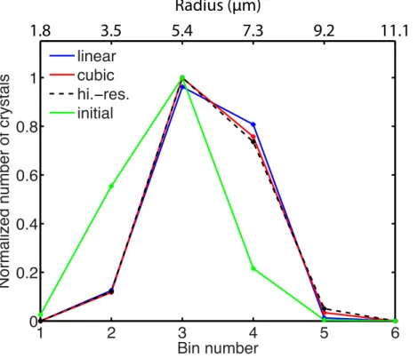
The supersaturation ratioSicedecreases from 0.40 at the initial time to 0.076 at 30 min.

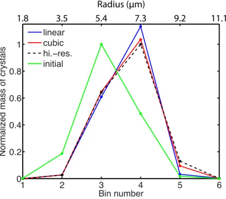
15

Numerical solutions at 6-bin-resolution at 30 min are shown in Fig. 3a (number of crystals per bin) and b (mass of crystals per bin). The solution obtained by the cubic scheme is more accurate than that by the linear scheme. At this resolution, the root-mean-square errors of the linear and cubic schemes are respectively 9.57_×103m−3 and 2.87_×103m−3 in crystal number and 1.67_×10−8kgm−3 and 0.50_×10−8kgm−3 20

(15)

ACPD

11, 21631–21654, 2011

Title Page

Tables Figures

◭ ◮

Back Close

Full Screen / Esc

Discussion

P

a

per

|

Dis

cussion

P

a

per

|

Discussion

P

a

per

|

Discussio

n

P

a

per

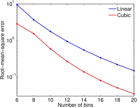
The errors of the solutions obtained by the linear and cubic schemes are given as a function of bin resolution in Table 2 and Fig. 4. The errors of the cubic scheme are typically about a third of those of the linear scheme.

The error reduction due to the cubic scheme means that the number of bins can be reduced without sacrificing accuracy. For the same accuracy, the number of bins 5

required for the cubic scheme is 20_±5 % less than that of the linear scheme. This is estimated as the difference in the intercepts of a horizontal line (whose value is the desired error) with the error curves of the cubic and linear schemes in Figs. 2 and 4.

4 Summary

We have presented a computationally efficient method to replace the piecewise linear 10

number distribution in the hybrid bin scheme originally developed by Chen and Lamb (1994) with a piecewise cubic polynomial. For models in which the CL scheme has been implemented, migrating from the linear distribution function to the cubic distribu-tion should be relatively simple.

When the original linear distribution is replaced by a cubic, the errors generated 15

in solutions to the condensation/evaporation equation are reduced by a factor of two to three. Alternatively, using the cubic distribution function would allow reducing the number of bins by 20_±5 % when solving the condensation/evaporation problem without sacrificing accuracy.

High bin resolution may be required for other microphysical processes besides con-20

(16)

ACPD

11, 21631–21654, 2011

Title Page

Tables Figures

◭ ◮

Back Close

Full Screen / Esc

Discussion

P

a

per

|

Dis

cussion

P

a

per

|

Discussion

P

a

per

|

Discussio

n

P

a

per

|

References

Chen, J. P. and Lamb, D.: Simulation of cloud microphysical and chemical processes us-ing a multicomponent framework. Part I: Description of the microphysical model, J. Atmos. Sci., 51, 2613–2613, doi:10.1175/1520-0469(1994)051<2613:SOCMAC>2.0.CO;2, 1994. 21632, 21634, 21636, 21645

5

Chen, J. P. and Lamb, D.: Simulation of cloud microphysical and chemical pro-cesses using a multicomponent framework. Part II: Microphysical evolution of a wintertime orographic cloud, J. Atmos. Sci., 56, 2293–2312, doi:10.1175/1520-0469(1999)056<2293:SOCMAC>2.0.CO;2, 1999. 21632

Dinh, T., Durran, D. R., and Ackerman, T.: Maintenance of tropical tropopause layer cirrus, J. 10

Geophys. Res., 115, D02104, doi:10.1029/2009JD012735, 2010. 21632

Hashino, T. and Tripoli, G. J.: The spectral ice habit prediction system (SHIPS). Part I: Model description and simulation of the vapor deposition process, J. Atmos. Sci., 64, 2210–2237, doi:10.1175/JAS3963.1, 2007. 21632

Kuba, N. and Fujiyoshi, Y.: Development of a cloud microphysical model and parameteriza-15

tions to describe the e_ffect of CCN on warm cloud, Atmos. Chem. Phys., 6, 2793–2810, doi:10.5194/acp-6-2793-2006, 2006. 21632

Kuba, N. and Murakami, M.: Effect of hygroscopic seeding on warm rain clouds - numeri-cal study using a hybrid cloud microphysinumeri-cal model, Atmos. Chem. Phys., 10, 3335–3351, doi:10.5194/acp-10-3335-2010, 2010. 21632

20

Lin, R.-F., Starr, D. O., Reichardt, J., and DeMott, P. J.: Nucleation in synoptically forced cirro-stratus,, J. Geophys. Res, 110, D08208, doi:10.1029/2004JD005362, 2005. 21632

Pruppacher, H. R. and Klett, J. D.: Microphysics of Clouds and Precipitation, D. Reidel Publish-ing Company, Dordrecht, Holland, 1978. 21643

Przyborski, P.: Goddard Cumulus Ensemble model, ONLINE, http://atmospheres.gsfc.nasa. 25

gov/cloud modeling/models gce.html, 2006. 21632

(17)

ACPD

11, 21631–21654, 2011

Title Page

Tables Figures

◭ ◮

Back Close

Full Screen / Esc

Discussion

P

a

per

|

Dis

cussion

P

a

per

|

Discussion

P

a

per

|

Discussio

n

P

a

per

Table 1.Root-mean-square errors in the number of drops (106m−3) of the solutions at 50 min

obtained by the linear and cubic schemes in the evaporation problem.

Number of bins Linear Cubic

(18)

ACPD

11, 21631–21654, 2011

Title Page

Tables Figures

◭ ◮

Back Close

Full Screen / Esc

Discussion

P

a

per

|

Dis

cussion

P

a

per

|

Discussion

P

a

per

|

Discussio

n

P

a

per

|

Table 2.Root-mean-square errors in the number of crystals (103m−3) of the solutions at 30 min

obtained by the linear and cubic schemes in the depositional growth problem.

Number of bins Linear Cubic

(19)

ACPD

11, 21631–21654, 2011

Title Page

Tables Figures

◭ ◮

Back Close

Full Screen / Esc

Discussion

P

a

per

|

Dis

cussion

P

a

per

|

Discussion

P

a

per

|

Discussio

n

P

a

per

10 12 14 16 18 20

0 0.2 0.4 0.6 0.8 1 1.2

Bin number

N

o

rma

lize

d

n

u

mb

e

r

o

f

d

ro

p

s

linear cubic exact initial

Radius (μm)

28

55

111

221

440

878

Fig. 1a. The analytical solution and numerical solutions obtained by the linear and cubic

(20)

ACPD

11, 21631–21654, 2011

Title Page

Tables Figures

◭ ◮

Back Close

Full Screen / Esc

Discussion

P

a

per

|

Dis

cussion

P

a

per

|

Discussion

P

a

per

|

Discussio

n

P

a

per

|

10 12 14 16 18 20

0 0.2 0.4 0.6 0.8 1 1.2

Bin number

N

o

rma

lize

d

ma

ss

o

f

d

ro

p

s

linear cubic exact initial

Radius (μm)

28

55

111

221

440

878

Fig. 1b. The analytical solution and numerical solutions obtained by the linear and cubic

(21)

ACPD

11, 21631–21654, 2011

Title Page

Tables Figures

◭ ◮

Back Close

Full Screen / Esc

Discussion

P

a

per

|

Dis

cussion

P

a

per

|

Discussion

P

a

per

|

Discussio

n

P

a

per

10 20 30 40 50 60 70 80 10−2

10−1 100

Number of bins

Root−mean−square error

Linear Cubic

Fig. 2. Root-mean-square errors in the number of drops (106m−3) of the solutions at 50 min

(22)

ACPD

11, 21631–21654, 2011

Title Page

Tables Figures

◭ ◮

Back Close

Full Screen / Esc

Discussion

P

a

per

|

Dis

cussion

P

a

per

|

Discussion

P

a

per

|

Discussio

n

P

a

per

|

1 2 3 4 5 6

0 0.2 0.4 0.6 0.8 1

Bin number

N

o

rma

lize

d

n

u

mb

e

r

o

f

cryst

a

ls

linear cubic hi.−res. initial

Radius (μm)

1.8

3.5

5.4

7.3

9.2

11.1

Fig. 3a.Numerical solutions obtained by the linear and cubic schemes at 30 min in the

(23)

ACPD

11, 21631–21654, 2011

Title Page

Tables Figures

◭ ◮

Back Close

Full Screen / Esc

Discussion

P

a

per

|

Dis

cussion

P

a

per

|

Discussion

P

a

per

|

Discussio

n

P

a

per

1 2 3 4 5 6

0 0.2 0.4 0.6 0.8 1

Bin number

N

o

rma

lize

d

ma

ss

o

f

cryst

a

ls

linear cubic hi.−res. initial

Radius (μm)

1.8

3.5

5.4

7.3

9.2

11.1

Fig. 3b. Numerical solutions obtained by the linear and cubic schemes at 30 min in the

(24)

ACPD

11, 21631–21654, 2011

Title Page

Tables Figures

◭ ◮

Back Close

Full Screen / Esc

Discussion

P

a

per

|

Dis

cussion

P

a

per

|

Discussion

P

a

per

|

Discussio

n

P

a

per

|

6 8 10 12 14 16 18 20

10−1

100

101

Number of bins

Root−mean−square error

Linear Cubic

Fig. 4. Root-mean-square errors in the number of crystals (103m−3) of the solutions at 30 min