www.geosci-model-dev.net/3/275/2010/
© Author(s) 2010. This work is distributed under the Creative Commons Attribution 3.0 License.
Geoscientific
Model Development
Modelling sediment export, retention and reservoir sedimentation in
drylands with the WASA-SED model
E. N. Mueller1, A. G ¨untner2, T. Francke1, and G. Mamede3 1Institute of Geoecology, University of Potsdam, Potsdam, Germany
2Helmholtz Centre Potsdam – GFZ German Research Centre for Geosciences, Potsdam, Germany
3Department of Environmental and Technological Sciences, Federal University of Rio Grande do Norte, Mossor´o, Brazil Received: 4 September 2008 – Published in Geosci. Model Dev. Discuss.: 2 October 2008
Revised: 19 November 2009 – Accepted: 22 March 2010 – Published: 8 April 2010
Abstract. Current soil erosion and reservoir sedimentation modelling at the meso-scale is still faced with intrinsic prob-lems with regard to open scaling questions, data demand, computational efficiency and deficient implementations of retention and re-mobilisation processes for the river and reservoir networks. To overcome some limitations of cur-rent modelling approaches, the semi-process-based, spatially semi-distributed modelling framework WASA-SED (Vers. 1) was developed for water and sediment transport in large dryland catchments. The WASA-SED model simulates the runoff and erosion processes at the hillslope scale, the trans-port and retention processes of suspended and bedload fluxes in the river reaches and the retention and remobilisation pro-cesses of sediments in reservoirs. The modelling tool en-ables the evaluation of management options both for sus-tainable land-use change scenarios to reduce erosion in the headwater catchments as well as adequate reservoir manage-ment options to lessen sedimanage-mentation in large reservoirs and reservoir networks. The model concept, its spatial discretisa-tion scheme and the numerical components of the hillslope, river and reservoir processes are described and a model ap-plication for the meso-scale dryland catchment Is´abena in the Spanish Pre-Pyrenees (445 km2) is presented to demonstrate the capabilities, strengths and limits of the model framework. The example application showed that the model was able to reproduce runoff and sediment transport dynamics of highly erodible headwater badlands, the transient storage of sedi-ments in the dryland river system, the bed elevation changes of the 93 hm3 Barasona reservoir due to sedimentation as well as the life expectancy of the reservoir under different management options.
Correspondence to:E. N. Mueller ([email protected])
1 Introduction
In drylands, water availability often relies on the retention of river runoff in artificial lakes and reservoirs. Such re-gions are exposed to the hazard that the available freshwa-ter resources fail to meet the wafreshwa-ter demand in the domes-tic, agricultural and industrial sectors. Erosion in the head-water catchments and deposition of the eroded sediments in reservoirs frequently threatens the reliability of reservoirs as a source of water supply. Erosion and sedimentation issues have to be taken into account when analysing and imple-menting long-term, sustainable strategies of land-use plan-ning (e.g. management of agricultural land) and water man-agement (e.g. reservoir construction and manman-agement). The typical scale relevant for the implementation of regional land and water management is often that of large basins with a size of several hundreds or thousands of square kilometres.
(Sivapalan et al., 1996) and SWAT (Neitsch et al., 2002). The latter, meso-scale modelling approaches often suffer from a problematic spatial representation of individual hillslope components in the headwater catchments, where most of the erosion occurs: the larger the modelling domain, the more averaging over spatial information occurs. The spatially semi-distributed SWAT model (Neitsch et al., 2002), for ex-ample, uses hydrologic response units to group input infor-mation in regard to land-use, soil and management combina-tions, thus averaging out spatial variations along the hillslope and topological information essential for sediment genera-tion and transport. In comparison, grid-based models such as the LISEM model (Jetten, 2002) may incorporate a higher degree of spatial information, but are often limited in their applicability due to computing time (for small grid sizes) and lack of exhaustive spatial data, which makes their application at the meso-scale inappropriate.
Both types of models fail to enable the quantification of sediment transfer from erosion hotspots of erosion, i.e. small hillslope segments that contribute a vast amount to the total sediment export out of a catchment but at the same time cover only a rather small part of the total area, such as badland hill-slopes or highly degraded hill-slopes which are often found in dryland settings (e.g. Gallart et al., 2002). Besides the spatial representation of erosion hotspots, current modelling frame-works often lack an integrated representation of all compo-nents of sediment transport in meso-scale basins, such as retention and transient storage processes in large reservoirs, reservoir networks and in a (potentially ephemeral) river net-work.
To enable regional land and water management with re-gard to sediment export in dryland settings, it was therefore decided to develop a sediment-transport model that:
– incorporates an appropriate scaling scheme for the spa-tial representation of hillslope characteristics to retain characteristic hillslope properties and at the same time is applicable to large regions (hundreds to thousands of km2);
– integrates sediment retention, transient storage and re-mobilisation descriptions for the river network (with a potential ephemeral flow regime) and large reservoirs and reservoir networks with the specific requirements of water demand and sedimentation problems of dryland regions;
– includes reservoir management options to calculate the life expectancy of reservoirs for different management practises; and
– is computationally efficient to cope with large spatial and temporal extent of model applications.
For this purpose, the WASA-SED (Water Availability in
Semi-Arid environments –SEDiments) model has been de-veloped and its structure, functioning and application is
pre-sented here. This paper describes the model as of March 2010 (Version 1, revision 30). It consists of two main parts: firstly, the numerical descriptions of the spatial representa-tion and the erosion and sediment transport processes in the hillslope, river and reservoir modules of WASA-SED are given. Secondly, a model application is evaluated for the Is´abena catchment (445 km2) in the Pre-Pyrenees, simulat-ing and discusssimulat-ing model performance and its limitations for badland hotspot erosion, transient storage of sediment in the riverbed, bed elevation change in the reservoir and manage-ment options for different life expectancies of a large reser-voir.
2 Numerical description of the WASA-SED model
2.1 Spatial representation of landscape characteristics
The WASA-SED model is designed for modelling at the meso-scale, i.e. for modelling domains of several hundreds to thousands of square kilometres. It uses a hierarchical top-down disaggregation scheme developed by G¨untner (2002) and G¨untner and Bronstert (2004) that takes into account the lateral surface and sub-surface flow processes at the hills-lope scale in a semi-distributed manner (Fig. 1). Each sub-basin of the model domain is divided into landscape units that have similar characteristics regarding lateral processes and resemblance in major landform, lithology, catena profile, soil and vegetation associations. Each landscape unit is rep-resented by a characteristic toposequence that is described with multiple terrain components (lowlands, slope sections and highlands) where each terrain component is defined by slope gradient, length, and soil and vegetation associations (soil-vegetation components). Within and between terrain components, the vertical fluxes for typical soil profiles con-sisting of several soil horizons and the lateral redistribution of surface runoff are taken into account.
(a)
(b)
Fig. 1.Spatial discretisation of the WASA-SED model (adapted after G¨untner, 2002): an example with 3 terrain components (TC) describing a catena and 4 landscape units (LU) describing a sub-catchment.
which allows to process and store digital soil, vegetation and topographical data in a coherent way and facilitates the gen-eration of the required input files for the model.
The advantage of the spatial concept in the WASA-SED model is that it captures the structured variability along the hillslope essential for overland flow generation and erosion. LUMP thus enables the incorporation of erosion hotspots in the parameterisation procedure. For example, the specific characteristics of small hillslope segments that exhibit ex-treme rates of erosion for geological or agricultural reasons can be retained in a large-scale model application. The up-scaling approach preserves a high degree of process-relevant details (e.g. intra-hillslope profile and soil distribution) while maintaining a slim demand in computational power and stor-age.
2.2 Hydrological module of the WASA-SED model
The hydrological model part of WASA-SED at the hillslope scale is fully described by G¨untner (2002) and G¨untner and Bronstert (2004). For daily or hourly time steps, the hydro-logical module calculates for each soil-vegetation component in each terrain component the following processes: inter-ception losses, evaporation and transpiration using the mod-ified Penman-Monteith approach (Shuttleworth and Wallace, 1985), infiltration with the Green-Ampt approach (Green and Ampt, 1911), infiltration-excess and saturation-excess runoff as well as its lateral redistribution between individual soil-vegetation components and terrain components, soil mois-ture and soil water changes for a multi-layer storage ap-proach, subsurface runoff and ground water recharge with a linear storage approach (G¨untner, 2002).
2.3 Sediment generation and transport processes in the hillslope module
The sediment module in WASA-SED provides four erosion equations of sediment generation by using derivatives of the
USLE equation (Wischmeier and Smith, 1978), which can be generalised as (Williams, 1995):
E=χ KLSC PROKFA (1)
whereEis erosion (t),Kthe soil erodibility factor
(t ha h ha−1MJ−1mm−1), LS the length-slope factor (–), C the vegetation and crop management factor (–),P the erosion control practice factor (–), ROKF the coarse fragment factor (–) as used in the USLE andAthe area of the scope (ha). χ is the energy term that differs between the USLE-derivatives, which are given below. It computes as (Williams, 1995):
USLE χ=EI
Onstad−Fosterχ=0.646EI+0.45(Qsurfqp)0.33 MUSLE χ=1.586(Qsurfqp)0.56A0.12 MUST χ=2.5(Qsurfqp)0.5
(2)
where EI is the rainfall energy factor (MJ mm ha−1h−1), Qsurfis the surface runoff volume (mm) andqpis the peak runoff rate (mm h−1). In contrast to the original USLE, the approaches (3–5) incorporate the surface runoffQsurf (calcu-lated by the hydrological routines) in the computation of the energy component. This improves the sediment modelling performance by eliminating the need for a sediment deliv-ery ratio (SDR) and implicitly accounts for antecedent soil moisture (Neitsch et al., 2002). Eis distributed among the user-specified number of particle size classes, according to the mean composition of the eroded horizons in the area.
E to obtain the sediment yield SY (t) of a terrain compo-nent. SY is limited by the transport capacityqs(t) of the flow leaving the terrain component:
SY=minimum(E+SEDin,qs) (3)
Two options are available to calculate the transport capacity qs:
(a) With the sediment transport capacity according to Ev-eraert (1991):
if D50≤150µm:qs=1.50×10−51.07D500.47W if D50>150µm:qs=3.97×10−61.75D−500.56W, with =(ρgpS)1.5/R2/3
(4) where is the effective stream power (g1.5s−4.5cm−2/3) computed within the hydrological routines of WASA-SED, D50is the median particle diameter (µm) estimated from the mean particle size distribution of the eroded soils andW is the width of the terrain component (m),ρis the density of the particles (g m−3),gis the gravitational acceleration (m s−2), q is the overland flow rate on a 1-m strip (m3s−1m−1) and Ris the flow depth (cm).
(b) With the maximum value that is predicted by MUSLE assuming unrestricted erodibility withKset to 0.5:
qs=EMUSLE,K=0.5 using Eq. (4) (5) Similar to the downslope partitioning scheme for surface runoff described by G¨untner and Bronstert (2004), sediment that leaves a terrain componenti is partitioned into a frac-tion that is routed to the next terrain component downslope (SEDin,TCi+1) and a fraction that reaches the river directly (SEDriver,i), representing the soil particles carried through
preferential flow paths, such as rills and gullies. SEDriver,i
is a function of the areal fractionαi of the current terrain i
component within the landscape unit according to:
SEDriver,i=SYi αi/ nTC
X
n=i αn
!
(6)
where i is the index of the current terrain component (counted from top),αis the areal fraction of a terrain com-ponent and nTC is the number of terrain comcom-ponents in the current landscape unit.
2.4 Transport and retention processes in the river module
The river network consists of individual river stretches with pre-defined river cross-sections. Each stretch is associated with one sub-basin, i.e., each stretch receives the water and sediment fluxes from one sub-basin and the fluxes from the upstream river network. The water routing is based on the
kinematic wave approximation after Muskingum (e.g. as de-scribed in Chow et al., 1988). Flow rate, velocity and flow depth are calculated for each river stretch and each time step using the Manning equation. A trapezoidal channel dimen-sion with widthw(m), depthd (m) and channel side ratio r (m m−1) is used to approximate the river cross-sections. If water level exceeds bankful depth, the flow is simulated across a pre-defined floodplain using a composite trapezoid with an upper width ofwfloodpl(m) and floodplain side ratio rfloodpl(m m−1). The WASA-SED river module contains rou-tines for suspended and bedload transport using the transport capacity concept. The maximum suspended sediment con-centration that can be transported in the flow is calculated using a power function of the peak flow velocity similar to the SWIM (Krysanova et al., 2000) and the SWAT model (Neitsch et al., 2002; Arnold et al., 1995):
Cs,max=a·vpeakb (7)
wherevpeak(t )is the peak channel velocity (m s−1),Cs,maxis the maximum sediment concentration for each river stretch in (ton m−3), andaandbare user-defined coefficients. If the actual sediment concentrationCactual exceeds the maximum concentration, deposition occurs; otherwise degradation of the riverbed is calculated using an empirical function of a channel erodibility factor (Neitsch et al., 2002):
RSEDdep = Cs,maxCactual·V
RSEDero = Cs,maxCactual·V·K·C
(8) where RSEDdep (ton) is the amount of sediment deposited, RSEDero (ton) the amount of sediment re-entrained in the reach segment (tons),V is the Volume of water in the reach (m3),Kis the channel erodibility factor (cm h−1Pa−1) and C is the channel cover factor (–). Using the approach af-ter Neitsch et al. (2002), it is possible to simulate the basic behaviour of a temporary storage and re-entrainment of sedi-ments in individual river segsedi-ments as a function of the trans-port capacity of the river.
Table 1.Bedload transport formulae in the river module.
Formula Range of conditions
1. Meyer-Peter and M¨uller (1948) for both uniform and non-uniform
qs=8(τ−τcrit)
1.5
gρ0.5 1000 sediment, grain sizes ranging from 0.4 to
with:τ=ρgdSandτcrit=0.047(ρs−ρ)gDm 29 mm and river slopes of up to 0.02 m m−1.
2. Schoklitsch (1950) for non-uniform sediment mixtures withD50
qs=2500S1.5(q−qcrit)1000ρsρ−sρ values larger than 6 mm and riverbed slopes
with:qcrit=0.26
ρ
s−ρ ρ
53D
3 2 50 S76
varying between 0.003 and 0.1 m m−1.
3. Smart and Jaeggi (1983) for riverbed slopes varying between
qs=4.2qS1.6
1−τcrit∗
τ∗
/
ρ
s ρ −1
1000(ρs−ρ) 0.03–0.2 m m−1andD
50values
with:τ∗= dS
ρs
ρ−1
D50
andτ∗ crit=
dcritS
ρs
ρ−1
D50
comparable to the ones of
the Meyer-Peter and M¨uller equation.
4. Bagnold (1956) reshaped by Yalin (1977), applicable for sand
qs=4.25τ∗0.5 τ∗
−τ∗ crit
ρs
ρ −1
gD5030.51000(ρs−ρ) and fine gravel and moderate riverbed slopes.
5. Rickenmann (2001) for gravel-bed rivers and torrents with bed
qs=3.1D90
D30
0.2
τ∗0.5 τ∗−τcrit∗ ·F r1.1ρs
ρ−1
−0.5ρ
s
ρ−1
gD503 0.51000(ρs−ρ) slopes between 0.03 and 0.2 m m−1and
with:F r=gv ·d
0.5
forD50values comparable to the ones
of the Meyer-Peter and M¨uller equation in the lower slope range with an averageD50
of 10 mm in the higher slope ranges.
d: mean water flow depth (m),dcrit: critical flow depth for initiation of motion (m),D50: median sediment particle size (m),D30:
grain-sizes at which 30% by weight of the sediment is finer (m),D90: grain-sizes at which 90% by weight of the sediment is finer (m),Dm: mean
sediment particle size (m),Fr: Froude number of the flow (–),g: acceleration due to gravity (m s−2),q: unit water discharge (m2s−1),
qcrit: unit critical water discharge (m2s−1),qs: sediment discharge in submerged weight (g ms−1),S: slope (m m−1),v: water flow velocity
(m s−1),ρ: fluid density (1000 kg m−3),ρs: sediment density (2650 kg m−3),τ: local boundary shear stress (kg ms−2),τcrit: critical local
boundary shear stress (kg ms−2),τ∗: dimensionless local shear stress (–),τ∗
crit: dimensionless critical shear stress (–).
2.5 Retention processes in the reservoir module
WASA-SED comprises a reservoir sedimentation module de-veloped by Mamede (2008). It enables the calculation of the trapping efficiency of the reservoir, sediment deposi-tion patterns and the simuladeposi-tion of several reservoir sediment management options and of reservoir life expectancy. The water balance and the bed elevation changes due to sedi-ment deposition or entrainsedi-ment are calculated for individual cross-sections along the longitudinal profile of the reservoir. Mamede (2008) subdivided the reservoir body (Fig. 2) in a river sub-reach component, where hydraulic calculations are based on the standard step method for a gradually varied flow (Graf and Altinakar, 1998) and a reservoir sub-reach com-ponent that uses a volume-based weighting factor approach adapted from the GSTARS model (Yang and Simoes, 2002). The transitional cross-section between the two spatial com-ponents is defined as where the maximum water depth for
uniform river flow, computed with the Manning equation, is exceeded by the actual water depth of the cross-section due to the impoundment of the reservoir. Consequently, the length of the river sub-reach becomes longer for lower reservoir lev-els and vice versa. For the reservoir routing, the water dis-chargeQjof each cross-sectionjis calculated as:
Qj=Qm−(Qin−Qout) j
X
k=m
vk with vk=Vk/Vres (9)
whereQin andQoutare reservoir inflow and outflow, vk is
the fraction of reservoir volume represented by the cross-section,Vresis the volume of the reservoir,Vk is the volume
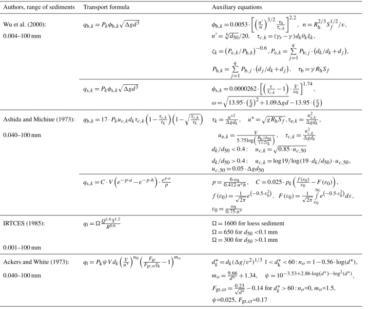
Table 2.Sediment transport formulae in the reservoir module.
Authors, range of sediments Transport formula Auxiliary equations
Wu et al. (2000): qb,k=Pkφb,k
p
1gd3 φ
b,k=0.0053·
n′ n
3/2 τ
b τc,k
2.2
, n=R2h/3Sf1/2/v ,
0.004–100 mm n′=√6d50/20, τc,k=(γs−γ )dkθkξk,
ζk= Pe,k/Ph,k
−0.6
,Pe,k= q
P
j=1
Pb,j· dk/dk+dj
,
Ph,k= q
P
j=1
Pb,j· dj/dk+dj, τb=γ RhSf
qs,k=Pkφs,k
p
1gd3 φ
s,k=0.0000262·
h
τ τc,k−1
·ωVk
i1.74
,
ω=
q
13.95· dv2
+1.091gd−13.95· dv
Ashida and Michiue (1973): qb,k=17·Pkuc,kdkτc,k
1−ττc,kk 1−
qτ
c,k
τk
τk= u∗ 2 1gdk, u
∗=p
gRhSf,τe,k= u2
e,k
1gdk,
0.040–100 mm ue,k= V
5.75logRh/d50 1+2τk
, τc,k=
u2
c,k
1gdk
dk/d50<0.4: uc,k=p0.85·uc,50
dk/d50>0.4: uc,k=log19/log(19·dk/d50)·uc,50, uc,50=0.05·1gd50
qs,k=C·V
e−p·a−e−p·h
·epp·a p=
6·ωk
0.412·u∗h, C=0.025·pk
f (ε0) ε0 −F (ε0)
,
f (ε0)=√12πe−0.5·ε 2 0
, F (ε0)=√12π ∞
R
ε0 e−0.5·ε02
dε,
ε0=0.75ωk·u∗ IRTCES (1985): qt=Q1.6S1.2
B0.6 =1600 for loess sediment
=650 ford50<0.1 mm =300 ford50>0.1 mm
0.001–100 mm
Ackers and White (1973): qt=Pkψ V dk
V u∗
n0 F
gr Fgr,crξk−1
mo
dk∗=dk(1g/v2)1/31< dk∗<60:no=1−0.56·log(d∗),
0.040–100 mm mo=9d.66∗ +1.34, ψ=10−3.53+2.86·log(d
∗)−log2(d∗),
Fgr,cr=0√.23
d∗−0.14 fordk∗>60:no=0,mo=1.5, ψ=0.025,Fgr,cr=0.17
qb,k: transport rate of thek-th fraction of bedload per unit width,qs,k: fractional transport rate of non-uniform suspended load,k: grain size class,Pk: ratio of material of size fractionkavailable in the bed,1: relative density (γ s/γ−1),γ andγs: specific weights of fluid and sediment, respectively;g: gravitational acceleration;dk: diameter of the particles in size class k,φb,k: dimensionless transport parameter
for fractional bed load yields,v: kinematic viscosity,τ: shear stress of entire cross-sectionτc,k: critical shear stress,θc: critical Shields parameter,ξk: hiding and exposure factor,Pe,k andPh,k: total exposed and hidden probabilities of the particles in size classk, Pb,j: probability of particles in size classjstaying in the front of particles in size classk,τb: average bed shear stress;n: manning’s roughness,
andn′: manning’s roughness related to grains,Rh: hydraulic radius,Sf:the energy slope,V: average flow velocity,d50: median diameter, ω: settling velocity,qt: total sediment transport capacity at current cross-section (qt=qs+qb, for the equations after Wu et al., 2000; Ashida and Michiue, 1973),S: bed slope, B: channel width,: constant as a function of grain size,u∗: shear velocity,uc,k: effective shear velocity,Fgr: sediment mobility number,no,mo,ψ,Fgr,crare dimensionless coefficients depending on the dimensionless particle sizedk∗, C: concentration at a reference level a.
The sediment transport is computed using a one-dimensional equation of equilibrium transport of non-uniform sediment, adapted from Han and He (1990):
dS dx=
αω
q S
∗−S
(10)
Fig. 2. Spatial discretisation of a reservoir along the longitudinal profile showing the river sub-reaches at cross-sections 1–7 and the main reservoir body at cross-sections 8–14. For each-cross-section, sediment deposition and re-entrainment is calculated for a control volume (as shown exemplarily for cross-section 11).
1.0 for scouring during flushing of a reservoir and in river channel with fine bed material. Mamede (2008) adapted four sediment transport equations (Wu et al., 2000; Ashida and Michiue, 1973; IRTCES, 1985; Ackers and White, 1973) for the calculation of the fractional sediment carrying capacity of both suspended sediments and bedload for different ranges of sediment particle sizes as given in Table 2.
The bed elevation changes of the reservoir are computed for each cross-section taking into account three conceptual layers above the original bed material: a storage layer, where sediment is compacted and protected against erosion; an in-termediate layer, where sediment can be deposited or re-suspended; and the top layer, where sediment-laden flow occurs. The time-dependent mobile bed variation is cal-culated using the sediment balance equation proposed by Han (1980):
∂(QS)
∂x +
∂M ∂t +
∂(ρdAd)
∂t =0 (11)
whereQis the water discharge;S is the sediment concen-tration; M is the sediment mass in the water column with unit length in longitudinal direction;Adis the total area of deposition, andρdis density of deposited material.
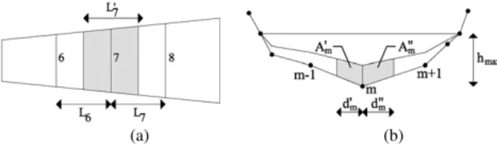
For each time step, the sediment balance is computed for each size fraction and cross-section, downstream along the longitudinal profile. The total amount of sediment deposited at each cross-section corresponds to the amount of sediment inflow exceeding the sediment transport capacity. On the other hand, the total amount of sediment eroded corresponds to the total amount of sediment that can still be transported by the water flux. Erosion is constrained by sediment availabil-ity at the bed of the reach. The geometry of the cross-section is updated whenever deposition or entrainment occurs at the intermediate layer. For each cross-section, the volume of sediments to be deposited is distributed over a stretch with a width of half the distance to the next upstream and down-stream cross-section, respectively (Fig. 3a). Suspended sedi-ment is assumed to be uniformly distributed across the cross-section and settles vertically, hence the bed elevationemat
(a) (b)
Fig. 3. Bed elevation change of a reservoir: (a)plan view along longitudinal profile: for each cross-section the volume of sediments to be deposited is distributed over a stretchL′7with a width of half the distance to the next upstream (CS 6 with a width ofL6) and
downstream (CS 8 with a width ofL8) cross-section,(b)deposition along an individual cross-section of the reservoir (for variables see Eq. 16).
a pointmalong the cross-section changes proportionally to water depth:
em=edep·fd,m (12)
whereedepis the maximum bed elevation change at the deep-est point of the cross-section caused by deposition andfd,m is a weighting factor which is computed as the ratio between water depthhmat the point m and the maximum water depth hmaxof the cross-section:
fd,m=hm/ hmax (13)
Figure 3b shows schematically, how the sediment is dis-tributed trapezoidally along the cross-section as a function of water depth hmax, whereA′m and A′′m are the sub-areas limited by the mean distances to the neighbour points (d′
m andd′′
m, respectively, starting from the deepest point of the cross-section profile), withmrunning from 1 tonwas the to-tal number of demarcation points of the cross-section below water level.
Bed entrainment is distributed in an equivalent way by as-suming a symmetrical distribution of bed thickness adapted from Foster and Lane (1983). The bed elevation change due to erosion is constrained by the maximum thickness of the intermediate layer. The bed elevation changeemis given by:
em=eero·fe,m (14)
whereeerois the maximum bed elevation change at the deep-est point of the cross-section caused by erosion andfe,mis a weighting factor given by Forster and Lane (1983):
fe,m=1−(1−Xm)2.9 (15)
whereXmis a normalised distance along the submerged half perimeter given by:
Xm=X/Xmax (16)
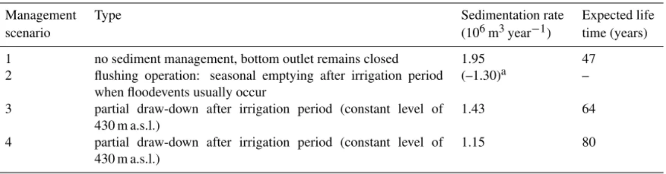
The implemented reservoir sedimentation routines allow the simulation of reservoir management options for the re-duction or prevention of sedimentation (Mamede, 2008), such as annual flushing operation or partial drawdown of the reservoir water level. Both management operations result in a remobilisation of previously deposited sediments and the release of sediments out of the reservoir. The management options can then be used to calculate the life expectancy of the reservoir by taking into account potential scenarios of water and land management for different land-uses and ero-sion prevention schemes in the upslope catchments. Besides the above sediment routine for individual large reservoirs, WASA-SED optionally provides a module to represent wa-ter and sediment retention processes within networks of farm dams and small reservoirs that often exist in large numbers in dryland areas. These mini-reservoirs cannot be represented explicitly each of them in a large-scale model because of data and computational constraints. Instead, WASA-SED applies a cascade structure that groups the reservoirs into different size classes according to their storage capacity, defines water and sediment routing rules between the classes and calcu-lates water and sediment balances for each reservoirs class. Details of the approach are presented with regard to water balance computations in G¨untner et al. (2004) and for related sedimentation processes in Mamede (2008).
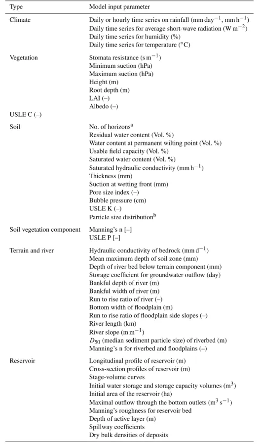
2.6 Summary of model input and output data
The model runs as a Fortran Console Application for catch-ment sizes of some tens to ten thousands of km2 on daily or hourly time steps. Climatic drivers are hourly or daily time series for precipitation, humidity, short-wave radiation and temperature. For model parameterisation, regional digi-tal maps on soil associations, land-use and vegetation cover, a digital elevation model with a cell size of 100 m (or smaller) and, optionally, data on reservoir geometry are required. The soil, vegetation and terrain maps are processed with the LUMP tool (see above) to derive the spatial discretisation into soil-vegetation units, terrain components and landscape units. Table 3 summarises the input parameters for the cli-matic drivers and the hillslope, river and reservoir modules. The vegetation parameters may be derived from the compre-hensive study of, for example, Breuer et al. (2003), the soil and erosion parameters with the data compilations of, e.g., FAO (1993, 2001), Morgan (1995), Maidment (1993) and Schaap et al. (2001), or from area-specific data sources.
The model output data are time series with daily or hourly time steps for lateral and vertical water and sediment fluxes from the sub-basins, the water and sediment discharge in the river network and the bed elevation change due to sedimen-tation in the reservoir as summarised in Table 4. A user’s manual for model parameterisation, the current version of LUMP and the source-code of WASA-SED as well as related tools can be used freely under the BSD-license, to be
down-Lower Isábena Villacarli
Cabecera
Barasona reservoir
0 2.5 5 7.5 10 km stream gauge
rain gauge
Ebro
42°20’N
0°30’E
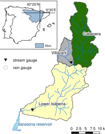
Fig. 4.Is´abena catchment and its sub-catchments.
loaded from http://brandenburg.geoecology.uni-potsdam.de/ projekte/sesam/reports.php.
3 Example application: modelling badland erosion, transient riverbed storage and reservoir
sedimentation for the Is´abena catchment
3.1 Study area and modelling objectives
The Is´abena catchment (445 km2) is located in the Central Spanish Pre-Pyrenees (42◦11′N, 0◦20′E). Climate is a typi-cal Mediterranean mountainous type with mean annual pre-cipitation rates around 770 mm. Heterogenous relief, lithol-ogy (Paleogene, Cretaceous, Triassic, Quaternary) and land-use (agriculture in the valley bottoms, mattoral, woodland and pasture in the higher parts) create a diverse landscape. Hotspot erosion occurs on badlands in the upper middle of the catchment, which is dominated by Mesozoic carbon-ate rocks and marls (Fig. 4). The Is´abena river never dries up, although flows are low during the summer (minimum flow: 0.45 m3s−1, mean annual discharge: Q
Table 3.Input data requirements for WASA-SED.
Type Model input parameter
Climate Daily or hourly time series on rainfall (mm day−1, mm h−1)
Daily time series for average short-wave radiation (W m−2)
Daily time series for humidity (%) Daily time series for temperature (◦C)
Vegetation Stomata resistance (s m−1)
Minimum suction (hPa) Maximum suction (hPa) Height (m)
Root depth (m) LAI (–) Albedo (–) USLE C (–)
Soil No. of horizonsa
Residual water content (Vol. %)
Water content at permanent wilting point (Vol. %) Usable field capacity (Vol. %)
Saturated water content (Vol. %)
Saturated hydraulic conductivity (mm h−1) Thickness (mm)
Suction at wetting front (mm) Pore size index (–)
Bubble pressure (cm) USLE K (–)
Particle size distributionb Soil vegetation component Manning’s n [–]
USLE P [–]
Terrain and river Hydraulic conductivity of bedrock (mm d−1)
Mean maximum depth of soil zone (mm) Depth of river bed below terrain component (mm) Storage coefficient for groundwater outflow (day) Bankful depth of river (m)
Bankful width of river (m) Run to rise ratio of river (–) Bottom width of floodplain (m)
Run to rise ratio of floodplain side slopes (–) River length (km)
River slope (m m−1)
D50(median sediment particle size) of riverbed (m)
Manning’s n for riverbed and floodplains (–)
Reservoir Longitudinal profile of reservoir (m)
Cross-section profiles of reservoir (m) Stage-volume curves
Initial water storage and storage capacity volumes (m3) Initial area of the reservoir (ha)
Maximal outflow through the bottom outlets (m3s−1) Manning’s roughness for reservoir bed
Depth of active layer (m) Spillway coefficients Dry bulk densities of deposits
Table 4.Model output files of WASA-SED.
Spatial unit Output (daily time series)
Sub-basins potential evapotranspiration (mm day−1) actual evapotranspiration (mm day−1) overland flow (m3timestep−1)
sub-surface flow
(m3timestep−1) groundwater discharge (m3timestep−1) sediment production (tons timestep−1) water content
in the soil profile (mm)
River water discharge (m3s−1) suspended sediment concentration (g l−1) bedload rate as submerged weight (kg s−1)
Reservoir sediment outflow from the reservoir (t timestep−1) bed elevation change due to deposition or erosion (m) storage capacity and sediment volume
changes (hm3) life expectancy (years) effluent size distribution of sediment (–)
Table 5.Geospatial data sources for Isbena case study.
Layer Source Author Resolution
Topography DEM generated from ASTER and SRTM data using stereo-correlation SESAM (unpublished) 30 m
Soils Mapa de suelos (Clasificacion USDA, 1987) CSIC/IRNAS (2000) 1:1 000 000
Lithology Geolog´ıa Dominio SINCLINAL DE TREMP; mapa “Fondos Aluviales” CHEBRO (1993) 1:50 000/200 000 Land use Usos de Suelos (1984/1991/1995) de la cuenca hidrogr´afica del Ebro CHEBRO (1998) 1:100 000
Badlands Digitized from high-resolution airphotos SESAM (unpublished) 1:5000
River stretches Field survey SESAM (unpublished) –
of suspended sediments that reach the reservoir via the ´Esera and Is´abena River. The badlands are considered to be the major cause for the sedimentation of the Barasona Reser-voir (Val´ero-Garces et al., 1999; Francke et al., 2008) whose initial capacity of 92 hm3has been considerably reduced by the subsequent siltation over the last several decades, thus threatening the mid-term reliability of irrigation water sup-ply (Mamede, 2008).
The WASA-SED model was used to simulate water and sediment fluxes from the hillslopes and suspended sediment transport in the river. Reservoir sedimentation dynamics were simulated separately with WASA-SED’s reservoir mod-ule. The simulation results were compared to discharge and suspended sediment concentration data at the catchment out-let and a headwater catchment containing large areas of bad-land formations (for details see Francke et al., 2008). Table 5 provides an overview of the data-sources used in the param-eterisation (for details, see Mamede, 2008; Francke, 2009).
With the highly heterogeneous landscape of the study area, modest data situation and the intense sediment export dy-namics caused by the badlands, the catchment poses a great challenge for any modelling. We propose that an adequate performance of the WASA-SED model in these settings is a strong indicator for its general applicability. On the other hand, the shortcomings of the model will become apparent. The model was employed to assess crucial questions for land and water management: a) how large is the runoff and
sedi-ment export from badland headwater catchsedi-ments and the en-tire Is´abena catchment, b) is there any transient times or tem-porary storage of sediments being delivered from the bad-lands to the outlet of the meso-scale catchment in the river system of the Is´abena, and c) what is the life expectancy of the Barasona reservoir under different management options.
High-resolution time series for water and sediment fluxes (1–10 min resolution) were available for a limited time pe-riod of one year at the outlets of the badland headwater Vil-lacarli (41 km2) and the entire Is´abena catchment. Several bathymetric surveys of the Barasona reservoir enabled a vali-dation of sedimentation rates along the longitudinal reservoir profile and for individual cross-sections.
3.2 Modelling runoff and erosion from highly erodible badlands and sediment fluxes at the catchment outlet of the Is´abena catchment
Table 6.Summary of model performance of the Is´abena.
Subcatchment Hydrological Sediment model
(modelled timespan) model
NS (%) SY (t) eSY(%)
Observed modelled
Villacarli 0.70 kern5.5mm74 000 kern5.5mm66 000 –11
(11 Sep 2006–30 Apr 2007)
Lower Is´abena 0.84 119 000 211 000 77
(15 Sep 2006–29 Jan 2007)
NS: Nash-Sutcliffe (1970) coefficient of efficiency; SY: sediment yield;eSY: relative error in modelled compared to observed sediment yield.
monitoring and modelling these fluxes is especially chal-lenging. The testing data sets were obtained during ex-tensive fieldwork as described in Francke et al. (2008) which defines the modelled time span (September 2006– January/April 2007).
The hydrological module of WASA-SED was able to re-produce the daily runoff dynamics of storm events for both the Villacarli badlands and the entire Is´abena catchment (Fig. 5) and yields Nash-Sutcliffe (1970) coefficients of ef-ficiency of 0.7 and 0.84, respectively (Table 6). The most pronounced deficit of the hydrological module was its fail-ure in correctly reproducing runoff peaks for certain events, which can be attributed to insufficient coverage of the spatial variation of rain storm events and unrepresented hydrologi-cal processes such as snowmelt. Furthermore, the temporal resolution of one day, which can only partly capture the ef-fects of high-intensity rainfall and restricts the reliability of the hydraulic computations, poses a limitation to model per-formance. The representation of low flow following a larger runoff event is affected by the simple modelling approach for groundwater in WASA-SED and the role of transmission losses, which could only rudimentarily be included in the pa-rameterization (Fig. 5).
For the sediment model, it was shown that the concept of combining runoff-driven erosion equations (Eqs. 4 and 5) and a transport capacity limitation (Eq. 6) yielded the best model performance, with only 11% underestimation in sed-iment yield (compared to observations, see Table 6) even for the badland-catchment Villacarli. WASA-SED reason-ably reproduced the total sediment yield of individual flood events (Fig. 6, note the logarithmic scale) that occurred after high-intensity rainstorm events in the autumn season. These events usually last one to three days and are responsible for the major part of sediments being transported through the river system. Figure 6 also illustrates that the observed sed-iment fluxes during low flow periods – a particularity of the Is´abena basin – were still underestimated for the badland headwater catchment, however well reproduced for the lower Is´abena catchment.
0
10
20
30
40
ra
in
fa
ll [
mm]
rainfall
01/10/06 01/11/06 01/12/06 01/01/07 0
20 40 60 80
di
s
c
har
ge [
m
3/s
] Q obs
Q sim
0
20
40
60
ra
in
fa
ll [
mm]
rainfall
01/09/060 01/11/06 01/01/07 01/03/07 5
10 15
di
s
c
h
ar
ge [
m
3/s
] Q obs
Q sim
Fig. 5. River discharge (Qobs: observed vs.Qsim: simulated) for
the Villacarli badlands (11 September 2006–30 April 2007, top) and the Is´abena (15 September 2006–29 January 2007, bottom) catch-ment.
3.3 Modelling the transient sediment storage in the lower Is´abena River
Figure 7 displays the temporal variation of the simulated sediment storage, i.e. sediments which were deposited dur-ing a runoff and erosion storm event and were stored in the riverbed of the lower section of the Is´abena catchment (Fig. 4) with a length of about 33 km for September 2006– January 2007.
100 101 102 103 104 105 10-2
100 102 104 106
sediment yield, obs [t]
s
edi
m
e
nt
y
iel
d
, s
im
[
t]
floods interfloods
100 101 102 103 104 105 106 100
101 102 103 104 105 106
sediment yield, obs [t]
s
edi
m
e
nt
y
iel
d
, s
im
[
t]
floods interfloods
Fig. 6.Flood-based sediment yield (observed vs. modelled) for the Villacarli (11 September 2006–4 January 2007, right) badlands and the Is´abena catchment (15 September 2006–29 January 2007, left).
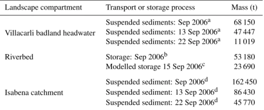
Table 7.Comparison of observed and modelled transient riverbed storage data with sediment fluxes of the Isabena and Villacarli catchments.
Landscape compartment Transport or storage process Mass (t)
Villacarli badland headwater
Suspended sediments: Sep 2006a 68 150 Suspended sediments: 13 Sep 2006a 47 447 Suspended sediments: 22 Sep 2006a 11 019
Riverbed Storage: Sep 2006b 53 180
Modelled storage 15 Sep 2006c 23 690
Isabena catchment
Suspended sediment: Sep 2006d 162 450 Suspended sediment: 13 Sep 2006d 86 430 Suspended sediment: 22 Sep 2006d 45 770
aderived from Francke et al. (2008) by taking their daily/monthly sediment flux values for a specific badland blinear interpolation of field data by Mueller (2008)
cderived from WASA-SED model, Fig. 7
dfrom Lopez-Tarazon et al. (2009), annual average: May 2005–May 2006: 90 410 t, May 2006–May 2007: 250 290 t, May 2007–May 2008:
212 070 t
1 10 100 1000 10000 100000
10/09/06 10/10/06 09/11/06 09/12/06 08/01/07
s
edi
m
ent
s
tor
age (
t)
0 10 20 30 40 50
dis
c
har
ge (
m
³/
s
)
sediment storage discharge
Fig. 7. Modelled discharge and sediment storage in the riverbed of the Lower Is´abena catchment (15 September 2006–29 January 2007).
catchment by subsequent storm events which often are much smaller than the storms which had caused the erosion in the badland area. A field study was carried out to quantify the transient riverbed storage of fine sediments of the Lower Is´abena River during the autumn period (first two weeks of
410 415 420 425 430 435 440 445 450
0 2000
4000 6000
8000 10000
Distance to the dam (m)
E
lev
ati
o
n
(
m
)
a
1986 measured 1993 measured Wu et al (2000a) IRTCES (1985)
Cross Section 40
430 440 450 460 470
100 300 500 700 900
x (m)
E
le
v
a
ti
on (
m
)
a initial
observed modelled
Cross Section 59
410 420 430 440 450 460 470
250 300 350 400 450 500
x (m)
E
le
v
a
ti
o
n
(m
)
a initial
observed modelled
0 1 2 3 4
1-0 2-1 3-2 4-3 5-4 6-5 7-6 8-7 9-8
Distance to the dam (km)
V
o
lu
m
e ch
an
g
es
(
h
m
3 )
observed modelled
Fig. 8.Measured and simulated bed elevation changes for the simulation period 1986–1993(a)along the longitudinal profile of the Barasona Reservoir for the Wu et al. (2000) and Tsinghua University (IRTCES, 1985) formulas;(b)at two different cross-sections for the Wu et al. (2000) formula;(c)Sediment volume changes along the longitudinal profile of the reservoir.
Table 8.Simulated life expectancy of the Barasona reservoir for four different management options.
Management Type Sedimentation rate Expected life
scenario (106m3year−1) time (years)
1 no sediment management, bottom outlet remains closed 1.95 47
2 flushing operation: seasonal emptying after irrigation period when floodevents usually occur
(–1.30)a –
3 partial draw-down after irrigation period (constant level of 430 m a.s.l.)
1.43 64
4 partial draw-down after irrigation period (constant level of 430 m a.s.l.)
1.15 80
Table 9.Summary of current WASA-SED model applications.
Processes Location Spatial scale Authors
Sediment export and land-use change mod-elling (afforestation, intensive agriculture, cli-mate change) from a Mediterranean catchment
Ribera Salada, Spain 65 km2 Mueller et al. (2009)
Connectivity investigation of sediment genera-tion and transport for a semi-arid catchment
Bengue, Brazil 933 km2 Medeiros et al. (2010)
Erosion of individual badland hillslopes Aragon, Spain ca. 10 ha Appel (2006)
Bedload modelling of a gravel-bed river Ribera Salada, Spain 65 and 222 km2 Mueller et al. (2008) Sedimentation and management options for the
Barasona reservoir
Aragon, Spain 1340 km2 Mamede (2008)
Sediment transport in a network of multiple small reservoirs
Bengue, Brazil 933 km2 Mamede (2008)
Surface runoff, river discharge and water avail-ability in reservoir networks
Cear´a, Brazil Up to several 10 000 km2 G¨untner and Bronstert (2004), G¨untner et al. (2004)
Comparing the order of magnitude of measured stored sediments in September 2006 (53 180 t for a river stretch of 33 km) with individual, monthly and annual sediment fluxes measured from the Villacarli and at the Is´abena outlets, the field data and the modelling results confirm that the riverbed storage can act as a sediment source for individual flood events as much as the hillslopes (Table 7 comparing the mea-sured suspended sediments for September 2006 and two indi-vidual events at the outlet of both catchments with the mea-sured and simulated transient storage in the riverbed). To ensure a sustainable river basin management, it is important to evaluate the relative importance of all involved sediment transport and storage compartments of a meso-scale catch-ment. This model application stresses the relative importance of the transient riverbed storage which was previously un-derrated for meso-scale sediment budgets of dryland catch-ments. At the moment it is possible to compare the modelled transient storage with one observation in time only (it took two weeks to collect the data set for the entire storage). More spatial and temporal variable field data on riverbed storage are required to enable an in-depth validation of its transfer behaviour.
3.4 Modelling sedimentation and management options for the Barasona reservoir
Mamede (2008) applied the reservoir module of the WASA-SED model to the Barasona Reservoir (location in Fig. 4) with a maximal storage capacity of 93 hm3 and a length of about 10 km using a total number of 53 cross-sections. Detailed bathymetric surveys were available for five years (1986, 1993, 1998, 2006, and 2007). They enable the pa-rameterisation of the cross-sections and the evaluation of bed elevation change over time and space.
The reservoir module was able to reproduce annual bed el-evation changes due to sedimentation of high-concentration
inflow both along the longitudinal profile and for individual cross-sections of the reservoir (Fig. 8a showing the longitudi-nal profile corresponding to the entire length of the Barasona Reservoir in Fig. 4, Fig. 8b showing the elevation changes for the time period 1986–1993). Figure 8c gives a quantita-tive comparison of measured and simulated sediment volume changes in a cumulative form (for 1 km segments). Overall, model deviations were less than 15%. However, consider-able differences occurred close to the reservoir inlet which may be explained by singularities of the reservoir topology (lateral constrictions and sharp bend of the narrow channel). A sensitivity analysis by Mamede (2008) showed that the WASA-SED reservoir module was sensitive to the choice of sediment transport equations (Fig. 8a shows that the IRTCES equation works slightly better than the Wu equation) and the number of cross-sections used. A coarser model discretiza-tion with, e.g., 14 instead of 53 cross-secdiscretiza-tions, slightly de-creased model performance, although not significantly.
4 Merits and limits of the WASA-SED model
The WASA-SED model is a new modelling framework for the qualitative and quantitative assessment of sediment trans-fer in large dryland catchments. The assets of the model are threefold:
First, the spatially detailed representation and scaling of catena characteristics using the landscape unit approach en-ables an effective way of parameterising large areas without averaging out topographic details that are particularly rele-vant for sediment transport. Crucial spatial information for the various sections of the catena, e.g., slope gradients, is pre-served. The semi-distributed approach of WASA-SED model therefore tends to be more adequate than raster-based erosion models at the meso-scale which for large cell sizes normally lack satisfactory aggregation methods for representing topo-graphic information when large cell sizes are employed to represent the often highly heterogeneous catenas of dryland catchments. Thus, simulated overland flow dynamics allow a realistic calculation of transport capacities and deposition patterns along the catena in WASA-SED.
Secondly, the WASA-SED framework allows a coherent handling of spatial input data in combination with the semi-automated discretisation tool LUMP (Francke et al., 2008). The tool provides an objective and easily reproducible de-lineation of homogeneous terrain components along a catena and consequently an upscaling rationale of small-scale hills-lope properties into the regional landscape units.
Thirdly, the WASA-SED model includes an integrative representation of various sediment processes in terms of hill-slope and river retention and transport, and of reservoir sed-imentation. Thus, different but closely interconnected sedi-ment transport and storage dynamics can be assessed at the river basin scale, including the effect of sediment manage-ment options both at hillslopes and in the river network. At the same time, the model maintains a slim demand in com-putational power and storage and is efficient enough to cope with data handling required for large catchments.
The source-code of WASA-SED can be used freely under the BSD-license, to be downloaded from http://brandenburg. geoecology.uni-potsdam.de/projekte/sesam//reports.php.
The example application for the Is´abena catchment has given quality measures for a range of modules of WASA-SED. The model was able to reproduce the runoff and ero-sion dynamics of a badland headwater catchment, gave new insight into the importance of a transient sediment storage of the lower riverbed, and quantified reservoir sedimenta-tion by calculating the spatial and temporal bed elevasedimenta-tion changes along a large reservoir. The Is´abena application re-vealed difficulties in reproducing the recession phase of the hydrographs and sedigraphs after storm events for the bad-land headwater catchment and at the outlet of the Is´abena catchment, which is due to a simplified modelling approach for transmission losses and groundwater processes. The val-idation of the simulated transient sediment storage in the
riverbed remains difficult, as no appropriate validation data are available for this process in recent literature.
The model was applied in several other studies to evaluate landscape and ecosystem functioning and the effects of land and reservoir management on the water and sediment export of large dryland catchments in Spain and north-eastern Brazil (see Table 9 for a summary of current applications). These studies include for example the assessment of spatial and temporal variability of water and sediment connectivity for a 933 km2dryland basin in the semi-arid northeast of Brazil (Medeiros et al., 2010), the analysis of bedload transport characteristics and ecosystem stability due to afforestation for a 65 km2mountainous catchment (Mueller et al., 2008, 2009) and the effects of a network of small reservoirs on water and sediment yield in a dryland catchment (Mamede, 2008). By reviewing the previous model applications (refer-ences in Table 8), several shortcomings of WASA-SED be-come apparent and recommend caution as with any model application at large scales. Uncertainties in process descrip-tions existed with regard to processes in inter-storm periods such as the soil moisture dynamics under different vegeta-tion cover (Mueller et al., 2009) and the erosion processes that are governed by the weathering, freezing and thawing cycles of the upper soil layer (Appel, 2006). In addition, the model contains only limited descriptions of processes which are commonly not regarded to be relevant for dryland set-tings, but may influence its hydrological regime under certain conditions, such as snow melt and groundwater movement as well as interaction and transmission losses in the riverbed (Francke, 2009).
Considering the merits and limits of WASA-SED, we be-lieve that WASA-SED is a powerful tool to assess erosion export dynamics at the meso-scale and could help to substan-tially improve the understanding of the processes that lead to reservoir sedimentation and the subsequent reduction of wa-ter availability in dryland environments.
Acknowledgements. This research was carried out within the
SESAM (Sediment Export from Semi-Arid Catchments: Mea-surement and Modelling) project and was funded by the Deutsche Forschungsgemeinschaft (DFG). Authors gratefully acknowledge the work done by two anonymous reviewers whose comments greatly improved the original version of the manuscript.
Edited by: D. Lunt
References
Ackers, P. and White, W. R.: Sediment transport: new approach and analysis, J. Hydr. Eng. Div.-ASCE, 99, 2041–2060, 1973. Appel, K.: Characterisation of badlands and modelling of
Arnold, J. G., William, J. R., Nicks, A. D., and Sammons, N. B.: SWRRB (A basin scale simulation model for soil and water re-sources management), User’s Manual, Texas A&M University Press, 195 pp., USA, 1989.
Arnold, J. G., Williams, J. R., and Maidment, D. R.: Continuous-time water and sediment-routing model for large basins, J. Hy-draul. Eng., 121, 171–183, 1995.
Bagnold, R. A.: The flow of cohesionless grains in fluids, Philos. T. R. Soc. Lond. A, 249, 235–297, 1956.
Batalla, R. J., Garcia, C., and Balasch, J. C.: Total sediment load in a Mediterranean mountainous catchment (the Ribera Salada River, Catalan Pre-Pyrenees, NE Spain), Z. Geomorphol., 49(4), 495–514, 2005.
Beven, K.: Rainfall-runoff modelling. The primer, John Wiley & Sons, Chichester, UK, 2001.
Boardman, J. and Favis-Mortlock, D.: Modelling soil erosion by-water, Series I: Global Environmental Change, Springer, Berlin, 55, 531 p., 1998.
Breuer, L., Eckhardt, K., and Frede, H.-G.: Plant parameter values for models in temperate climates, Ecol. Model., 169, 237–293, 2003.
CHEBRO: La Confederacion hidgroafica del Ebro, Zaragoza, Spain, 2002 (in Spanish).
CHEBRO: Mapa “Fondos Aluviales” 1:50 000, available at: http: //www.chebro.es/ContenidoCartoGeologia.htm (last access: 1 April 2010), 1993 (in Spanish).
CHEBRO: Usos de Suelos (1984/1991/1995) de la cuenca hidro-grafica del Ebro; 1:100 000, Consultora de M. Angel Fern´andez-Ruffete y Cereyo, Oficina de Planificaci´on Hidrol´ogica, C.H.E., available at: http://www.chebro.es/ (last access: 1 April 2010), 1998 (in Spanish).
CSIC/IRNAS: Mapa de suelos (Clasificacion USDA, 1987), 1:1 Mio, Sevilla, SEISnet-website, available at: http://www.irnase. csic.es/ (last access: 1 April 2010), 2000 (in Spanish).
Chow, V. T., Maidment, D. R., and Mays, L. W.: Applied Hydrol-ogy, in: Civil Engineering Series, McGraw-Hill Int. eds., Singa-pore, 1988.
De Roo, A. P. J., Wesseling, C. G., and Ritsema, C. J.: LISEM: a single event physically-based hydrologic and soil erosion model for drainage basins. I: Theory, input and output, Hydrol. Pro-cesses, 10, 1107–1117, 1996.
Everaert, W.: Empirical relations for the sediment transport capac-ity of interrill flow, Earth Surf. Proc. Land., 16, 513–532, 1991. FAO: Global and national soils and terrain digital databases
(SOTER), Procedures Manual, World Soil Resources Reports, No. 74., FAO (Food and Agriculture Organization of the United Nations), Rome, Italy, 1993.
FAO: Global Soil and Terrain Database (WORLD-SOTER), FAO, AGL (Food and AgricultureOrganization of the United Nations, Land and Water Development Division), available at: http:// www.fao.org/ag/AGL/agll/soter.htm., 2001.
Foster, G. R. and Wischmeier, W. H.: Evaluating irregular slopes for soil loss prediction, T. ASAE, 17, 305–309, 1974.
Francke, T., G¨untner, A., Bronstert, A., Mamede, G., and M¨uller, E. N.: Automated catena-based discretisation of landscapes for the derivation of hydrological modelling units, Int. J. Geogr. Inf. Sci., 22, 111–132, 2008.
Francke, T., L´opez-Taraz´on, J. A., Vericat, D., Bronstert, A., and Batalla, R. J.: Flood-Based Analysis of High-Magnitude
Sed-iment Transport Using a Non-Parametric Method, Earth Surf. Proc. Land., 33(13), 2064–2077, 2008.
Francke, T.: Measurement and Modelling of Water and Sediment Fluxes in Meso-Scale Dryland Catchments, Ph.D. thesis, Uni-versit¨at Potsdam, Potsdam, available at: http://nbn-resolving.de/ urn:nbn:de:kobv:517-opus-31525, 2009.
Gallart, F., Sol´e, A., Puigdef´abregas, J., and L´azaro, R.: Badland Systems in the Mediterranean, in: Dryland rivers, edited by: Bull, L. J. and Kirkby, M. J., Hydrology and Geomorphology of Semi-arid Channels, 299–326, 2002.
Graf, W. H. and Altinakar, M. S.: Fluvial hydraulics – flow and transport processes in channels of simple geometry, John Wiley & Sons LTDA, ISBN 0-471-97714-4, 1998.
Green, W. H. and Ampt, G. A.: Studies on soil physics I. The flow of air and water through soils, J. Agr. Sci, 4, 1–24, 1911. G¨untner, A.: Large-scale hydrological modelling in the semi-arid
North-East of Brazil, Dissertation, Institut f¨ur Geo¨okologie, Uni-versit¨at Potsdam, PIK-Report, Nr. 77, 2002.
G¨untner, A. and Bronstert, A.: Representation of landscape vari-ability and lateral redistribution processes for large-scale hydro-logical modelling in semi-arid areas, J. Hydrol., 297, 136–161, 2004.
G¨untner, A., Krol, M. S., Ara´ujo, J. C. d., and Bronstert, A.: Sim-ple water balance modelling of surface reservoir systems in a large data-scarce semiarid region, Hydrol. Sci. J., 49(5), 901– 918, 2004.
Haan, C. T., Barfield, B. J., and Hayes, J. C.: Design hydrology and sedimentology for small catchments, Academic Press, San Diego, CA, 1994.
Han, Q. W.: A study on the non-equilibrium transportation of sus-pended load, Proc. Int. Symps. on River Sedimentation, Beijing, China, 2, 793–802, 1980.
Han, Q. and He, M.: A mathematical model for reservoir sedi-mentation and fluvial processes, Int. J. Sediment Res., 5, 43–84, 1990.
IRTCES: Lecture notes of the training course on reservoir sedimen-tation. International Research of Training Center on Erosion and Sedimentation, Sediment Research Laboratory of Tsinghua Uni-versity, Beijing, China, 1985.
Jetten, V.: LISEM user manual, version 2.x. Draft version January 2002. Utrecht Centre for Environment and Landscape Dynamics, Utrecht University, The Netherlands, 48 pp., 2002.
Kirkby, M. J.: Physically based process model for hydrology, ecol-ogy and land degradation, in: Mediterranean Desertification and Land Use, edited by: Brandt, C. J. and Thornes, J. B., Wiley, UK, 1997.
Krysanova, F., Wechsung, J., Arnold, R., Srinivasan, J., and Williams, J.: SWIM (Soil and Water Integrated Model), User Manual, PIK Report Nr. 69, 239 pp., 2000.
L´opez-Taraz´on, J. A., Batalla, R. J., Vericat, D., and Francke, T.: Suspended sediment transport in a highly erodible catch-ment: The river Isabena (Central Pyrenees), Geomorphology, 109, 210–221, 2009.
Mamede, G.: Reservoir sedimentation in dryland catchments: Mod-elling and management, PhD thesis, University of Potsdam, Germany, published on: http://opus.kobv.de/ubp/volltexte/2008/ 1704/, 2008.
Medeiros, P., Guntner, A., Francke, T., Mamede, G., and de Araujo, J. C.: Modelling spatio-temporal patterns of sediment yield and connectivity in a semi-arid catchment with the WASA-SED model, Hydrol. Sci. J., accepted, 2010.
Meyer-Peter, E. and M¨uller, R.: Formulas for bedload transport, Proc. International Association of Hydraulic Research, 3rd An-nual Conference, Stockholm, 39–64, 1948.
Morgan, R. P. C.: Soil erosion and conservation Longman Group, UK, Limited, 304 pp., 1995.
Morgan, R. P. C., Quinton, J. N., Smith, R. E., Govers, G., Poesen, J. W. A., Auerswald, K., Chisci, G., Torri, D., and Styczen, M. E.: The European Soil Erosion Model (EUROSEM): a dynamic approach for predicting sediment transport from fields and small catchments, Earth Surf. Proc. Land., 23, 527–544, 1998. M¨uller, E. N., Batalla, R. J., and Bronstert, A. Dryland river
mod-elling of water and sediment fluxes using a representative river stretch approach, Book chapter IN: Natural Systems and Global Change, German-Polish Seminar Turew, Poznan, 2006. Mueller, E. N., Francke, T., Batalla, R. J., and Bronstert, A.:
Mod-elling the effects of land-use change on runoff and sediment yield for a meso-scale catchment in the Southern Pyrenees, CATENA, 79, 288–296, 2009.
Mueller, E. N., Batalla, R. J., Garcia, C., and Bronstert, A.: Mod-elling bedload rates from fine grain-size patches during small floods in a gravel-bed river, J. Hydrol. Eng., 134, 1430–1439, 2008.
Mueller, E. N.: Quantification of transient sediment storage in the riverbed for a dryland setting in NE Spain, SESAM Internet Resources, available at: http: //brandenburg.geoecology.uni-potsdam.de/projekte/sesam/ download/Projects/Project Transient Sediment Storage.pdf, 2008.
Nash, J. E. and Sutcliffe, V.: River flow forecasting through concep-tual models, I. A discussion of principles, J. Hydrol., 10, 282– 290, 1970.
Neitsch, S. L., Arnold, J. G., Kiniry, J. R., Williams, J. R., and King, K. W.: Soil and Water Assessment Tool, Theoretical Doc-umentation, Version 2000, Published by Texas Water Resources Institute, TWRI Report TR-191, 2002.
Quinton, J.: Erosion and sediment transport, Book chapter in: Find-ing simplicity in complexity, edited by: Wainwright, J. and Mul-ligan, M., Environmental Modelling, John Wiley & Sons, Chich-ester, UK, 2004.
Rickenmann, D.: Comparison of bed load transport in torrents and gravel bed streams, Water Resour. Res., 37, 3295–3305, 2001.
Schaap, M. G., Leij, F. J., and van Genuchten, M. Th.: ROSETTA: a computer program for estimating soil hydraulic parameters with hierarchical pedotransfer functions, J. Hydrol., 251, 163–176, 2001.
Schmidt, J.: A mathematical model to simulate rainfall erosion, Catena Suppl., 19, 101–109, 1991.
Schoklitsch, A.: Handbuch des Wasserbaus, 2nd edn., Springer, Vi-enna, 257 pp., 1950.
Shuttleworth, J. and Wallace, J. S.: Evaporation from sparse crops – an energy combination theory, Q. J. Roy. Meteorol. Soc., 111, 839–855, 1985.
Sivapalan, M., Viney, N. R., and Jeevaraj, C. G.: Water and salt balance modelling to predict the effects of land use changes in forested catchments. 3. The large scale model, Hydrol. Processes, 10, 429–446, 1996.
Smart, G. M. and Jaeggi, M. N. R.: Sediment transport on steep slopes, Mitteil. 64, Versuchsanstalt f¨ur Wasserbau, Hydrologie und Glaziologie, ETH-Z¨urich, Switzerland, 1983.
Sidorchuk, A.: A dynamic model of gully erosion, in: Mod-elling soil erosion by water, edited by: Boardman, J. and Favis-Mortlock, D., NATO-Series I, Berlin, Heidelberg, 55, 451–460, 1998.
Sidorchuk, A. and Sidorchuk, A.: Model for estimating gully mor-phology, IAHS Publ., Wallingford, 249, 333–343, 1998. USDA-SCS: USDA-SCS, Ephemeral Gully Erosion Model.
EGEM. Version 2.0 DOS User Manual, Washington, 1992. Valero-Garc´es, B. L., Navas, A., Mach´ın, J., and Walling, D.: Sediment sources and siltation in mountain reservoirs: a case study from the Central Spanish Pyrenees, Geomorphology, 28, 23–41, 1999.
Von Werner, K.: GIS-orientierte Methoden der digitalen Reliefanal-yse zur Modellierung von Bodenerosion in kleinen Einzugsge-bieten, Dissertation, Inst. f. Geographische Wissenschaften, TU Berlin, 1995.
Williams, J.: The EPIC Model, in: Computer Models of Watershed Hydrology, edited by: Singh, V. P., Water Resources Publica-tions, Highlands Ranch, CO, 909–1000, 1995.
Wu, W., Rodi, W., and Wenka, T.: 3-D numerical modeling of flow and sediment transport in open channels, J. Hydrol. Eng., 126, 4–15, 2000.
Wischmeier, W. and Smith, D.: Predicting rainfall erosion losses, US Gov. Print. Off, Washington, 1978.