Air Quality Assessment Using Interpolation Technique
Awkash Kumar a, Rashmi S. Patil a, Anil Kumar Dikshit a and Rakesh Kumar b
a
Centre for Environmental Science and Engineering, Indian Institute of Technology Bombay, Mumbai-400076, India
b
National Environmental Engineering Research Institute Mumbai Zone, Mumbai-400018, India
Abstract
Air pollution is increasing rapidly in almost all cities around the world due to increase in population. Mumbai city in India is one of the mega cities where air quality is deteriorating at a very rapid rate. Air quality monitoring stations have been installed in the city to regulate air pollution control strategies to reduce the air pollution level. In this paper, air quality assessment has been carried out over the sample region using interpolation techniques. The technique Inverse Distance Weighting (IDW) of Geographical Information System (GIS) has been used to perform interpolation with the help of concentration data on air quality at three locations of Mumbai for the year 2008. The classiication was done for the spatial and temporal variation in air quality levels for Mumbai region. The seasonal and annual variations of air quality levels for SO2, NOx and SPM (Suspended Particulate Matter) have been focused in this study. Results show that SPM concentration always exceeded the permissible limit of National Ambient Air Quality Standard. Also, seasonal trends of pollutant SPM was low in monsoon due rain fall. The inding of this study will help to formulate control strategies for rational management of air pollution and can be used for many other regions.
Keywords: air quality; interpolation technique; ArcGIS; IDW
1. Introduction
Urbanization is a major trend all over the world mainly due to rapid growth in population. More than half the population of the world now lives in urban areas. This may be attributed to the continuous increase in global population (Kim, 2005; Huff and Angeles, 2011). Urbanization is affecting air quality at global, regional and local scales (Contini et al., 2012; Duh et al., 2008; Nemitz et al., 2008; Järvi et al., 2009). Urban air quality is a complex subject with different socio-economic aspects in different parts of the world and even within a specific region. The population growth is directly correlated to many environmental quality parameters like water and air quality (Alcamo et al., 2002; Bollen et al., 2009; 2010; Kan et al., 2012; Kanada et al., 2013; Yennawar, 1978). Nowadays air pollution is becoming a major issue in urban areas especially megacities such as Mumbai, Delhi, and Chennai in India. It has many sources like vehicles, industries, bakeries, domestic sector, load from cremation and hotels. Mumbai is the capital of the state of Maharashtra and is the most populated city in India. Furthermore, it is the inancial, commercial and entertainment capital of India with the total population of more than eighteen million people (Census, 2011).
Air quality studies are done with monitoring and modeling techniques (Gulia et al., 2015; Kumar
et al., 2015; Li et al., 2011). Air quality modeling requires emission data, meteorological data and surface characteristics for the region, collecting which can prove to be rigorous and tedious. Air quality monitoring is carried out by many authorities to communicate air quality status and this data can be easily collected. The monitoring data is a combination of emission sources and meteorological data which represents air quality status at a point. The objective of this study is to understand the air quality status through the use of interpolation techniques leading to delineating of spatial pattern over a region. The outcome of the study will signiicantly help in air pollution management, wherein a small dataset can be used for air quality mapping of a larger area. The study has been carried out in three locations within the Mumbai city to analyse air quality. ArcGIS was used to interpolate these values over the Mumbai region for the year 2008. Many communities and regulatory authorities have installed air quality monitoring stations to communicate air quality level or as a part of research and development. National Environmental Engineering Research Institute (NEERI) is a government organisation working continuously to ascertain the critical conditions of environment
The international journal published by the Thai Society of Higher Education Institutes on Environment
E
nvironment
A
sia
EnvironmentAsia 9(2) (2016) 140-149
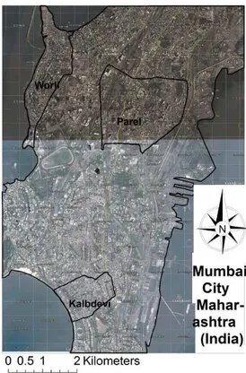
141 and suggest control options for the environmental problems. NEERI measures ambient air quality concentration at three locations in the Mumbai region namely Kalbadevi, Worli and Parel. In the present study, concentration data-sets at three locations have been interpolated over the Mumbai region and interpolated spatial and seasonal patterns have been observed that can help in rational management of air quality. The study area “Mumbai city” is depicted Fig. 1 where the three stations Parel, Kalbadevi and Worli are presented. Parel is situated in central Mumbai and represents an inlux of huge enterprises in the compounds of the long-gone cotton mills. K a l b a d e v i i s a r e s i d e n t i a l a r e a a n d a n o l d neighbourhood in Mumbai. Worli is a part of South Mumbai and is one of the original seven islands that constituted the Mumbai city. Now, it has become one of the busiest ofice areas in the city.
2. Methodology
2.1 Geographical Information System (GIS) and its applications
Geographical Information System (GIS) is an eficient tool to capture, store, manipulate, manage, and analyse various types of geographical data and represent graphical view for easy understanding. ArcGIS software has several inbuilt tools which
include many operations such as interpolation techniques, network analysis and spatial analysis. ArcGIS is widely used for modeling and simulation using data processing and various mathematical functions. This tool can help to estimate the levels of air pollution at various locations of the study region. This estimation is very useful to formulate control strategies for air quality management. ArcGIS has been applied in several studies for assessing air quality and exposure (Gulliver and Briggs, 2011; Cinderby and Forrester, 2005; Ketzel et al., 2011; Jensen et al., 2001; Kumar et al., 2016; Maantay, 2007; Marquez and Smith, 1999; Pummakarnchana
et al., 2005; Sohrabinia and Khorshiddoust, 2007; Vienneau et al., 2009; Wang et al., 2009; Zhang et al., 2008). There are many interpolation techniques available in ArcGIS such as Kriging, Spline and Inverse Distance Weighting (IDW). Interpolation techniques are considered good tools to study spatial and temporal patterns of air quality without requiring data on meteorology and emissions (Candiani et al., 2013; Janssen et al., 2008; van Loon, 1993). The urban Indian case studies show that Inverse Distance Weighting gives a fairly good performance for the interpolation of the concentration of air pollutants as compared to other interpolation techniques, because the regional and local aspects both are incorporated. The evaluation of IDW interpolation technique for the concentration of ambient air quality in Port Blair
142 (India) has been reported by Jha et al. (2011). Wong
et al. (2004) have also demonstrated that IDW gives fairly good interpolation of air quality (Kumar
et al., 2016). IDW interpolates all values of the points within the sample range as averaging tool and gives better interpolation estimates when the minimum and maximum values of the surface are represented by sample data points. It estimates the value of a point as a basis of a function of two variables: the distance between sampling points and the point at which the value has to be estimated. The concentration of point will have heavier weight if it is proximal to the required point and vice versa. Here, weight is an inverse function of the distance, as demonstrated in the following equation:
Eq 1.
where Zj is the value of concentration at the j th
point, Wi is the weight of observed i
th
point, dji is the distance from the ith point to the jth point, p is the power and n is total number of points.
A base map was taken and geo-referencing was done to associate with physical earth space in ArcGIS. Shapefiles were created with the help of the geo-referenced map for air quality monitoring stations and for the Mumbai region. The air quality monitoring locations are denoted by point shapeile and area of south-west Mumbai is denoted by polygon shapile in Mumbai region. Air quality data, monitored by NEERI (Mumbai), was fed in the attribute of point
shapefiles on the basis of monthly, seasonal and annual average. Colorimetric method for SO2, NOx and gravimetric method for SPM were used to monitor air quality data with the help of High Volume Sampler. The monitoring station runs for twice a week and collect 104 data in a year as per (National Ambient Air Quality Standard) NAAQS. The Inverse Distance Weighting (IDW) was used to interpolate the data of three point shapeiles for the concentrations of SO2, NOx and SPM in the study area.
3. Results and Discussion
3.1 Results of monitoring data
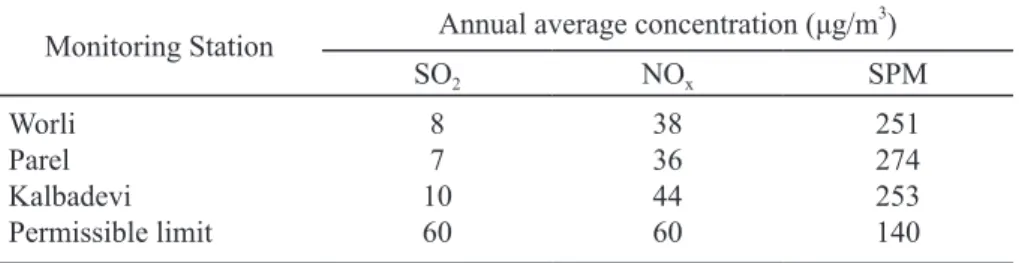
Based on monitored data-set of ambient concentration at three locations, it can be concluded that the annual average concentration of SO2 and NOx is low while concentration of SPM is consistently high all over Mumbai region for the year 2008. The annual permissible limits of NAAQS by Central Pollution Control Board (CPCB) are 60 μg/m3 for SO2 and NOx and 140 μg/m
3
for SPM (CPCB, 2008).Annual average values of the air quality parameters considered in this study are shown in Fig. 2. The maximum annual average concentrations of SO2 and NOx are found to be 10 and 44 μg/m
3 in Kalbadevi amongst the three locations, which are well below the standards. Annual average concentrations of SO2 and NOx are close to these values at Parel and Worli: 7 and 36 μg/m3
, respectively. The annual average concentrations of SPM is 251, 253 and 274 μg/m3
at Worli, Kalbadevi and Parel, respectively, which is above the permissible limit.
on:
and
here Z is the value of concentration at the
∑
∑
= =
=
ni i n
i i i
j
W
Z
W
Z
1 1
p ji i
d
W
=
1
M M M
16 70 323 24 74 414 14 62 410
Figure 2. Annual average concentration (μg/m3
143 Table 1 enlists the annual values for the three stations and permissible limit values for the three pollutants, which have been provided by CPCB. The SPM concentration at all three locations is higher than the CPCB standard. Table 2 shows seasonal concentrations of three pollutants at the three stations. The SO2 concentration is maximum at Kalbadevi from the post-monsoon to winter season which shows industrial emission effect. Worli and Parel have higher concentration for SPM in the monsoon which may be because of resuspension of dust. Kalbadevi and Parel have maximum concentration in the winter. Table 3 shows monthly concentrations of three pollutants at the three stations in which daily standard of air quality of pollutants have been included. Ambient air quality standards are not included in Table 2 because standards are given only on a daily and annual basis. It is evident that SPM exceeds the permissible limit of air quality standard at all three locations while the other two parameters (SO2 and NOx) are within limits. The monthly concentration of SPM at all three locations are within limits in the monsoon season because of washout due to rainfall.
Figs. 3 (a), (b) and (c) show bar plots of seasonal average concentration for air pollutants SO2, NOx and SPM at the three monitoring sites respectively. Seasons are considered as follows: December and January represent the winter season, February, March, April and May are the pre-monsoon season, June, July, August and September are the monsoon months and the post-monsoon season comprises of October
and November. Seasonal average concentrations of SO2, NOx and SPM were highest in the winter season, and maximum seasonal concentrations were observed at Kalbadevi for SO2, NOx and SPM (24, 76 and 414 μg/m3
, respectively). SPM concentrations were high in each season except during monsoon at Worli and Parel. It may be because these are dense and congested regions where resuspension of particulate matter occurs more. Figs. 4 (a), (b) and (c) represent monthly variations of SO2, NOx and SPM, respectively, for the year 2008. The concentration of pollutants was found to start decreasing from winter season to pre-monsoon season and concentrations of all pollutants was least in the monsoon season.
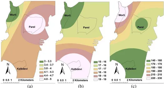
3.2 Results of IDW interpolation
The collected monitored dataset was used in ArcGIS 9.3 to interpolate the concentration data-set of air quality using IDW. Figs. 5 to 9 show the results of use of IDW interpolation technique. Figs. 5 (a), (b) and (c) show contour plots of annual average for air pollutants SO2, NOx and SPM respectively. Annual average concentrations of SO2 and NOx are maximum at Kalbadevi, but SPM is higher in Parel at 274 μg/m3
. In these igures, spatial patterns indicate that NOx and SO2 may be transported from Kalbadevi to Worli and from Worli to Parel, However, in the case of SPM, pollutant may be transported from Parel to Worli and Kalbadevi over the year.
Table 1. Annual values for the three stations and permissible limit values for the three pollutants
M M M
16 70 323 24 74 414 14 62 410
36 231 36 259 32 296
15 226 19 142 16 151
10 58 269 14 71 300 51 343
Locations/ Worli Kalbadevi Parel
Season SO2 NOx SPM SO2 NOx SPM SO2 NOx SPM
Winter 16 70 323 24 74 414 14 62 410
Premonsoon 9 36 231 8 36 259 8 32 296
Monsoon 3 15 226 4 19 142 3 16 151
Postmonsoon 10 58 269 14 71 300 7 51 343
Table 2. Seasonal concentrations (μg/m3
) of three pollutants at the three stations Monitoring Station Annual average concentration (μg/m
3 )
SO2 NOx SPM
Worli Parel Kalbadevi Permissible limit
8 7 10 60
38 36 44 60
144
Locations/ Worli Kalbadevi Parel Standard (Daily)
Pollutants SO2 NOx SPM SO2 NOx SPM SO2 NOx SPM SO2 NOx SPM
JAN 18 68 322 23 64 397 15 64 436 80 80 200
FEB 14 56 345 13 60 398 13 39 417 80 80 200
MAR 9 40 209 10 39 261 8 37 273 80 80 200
APR 9 30 228 8 28 249 7 33 296 80 80 200
MAY 4 17 142 2 17 127 4 20 196 80 80 200
JUN 2 13 207 3 16 147 2 15 176 80 80 200
JUL 2 9 211 3 16 147 3 12 138 80 80 200
AUG 3 13 285 3 17 127 3 15 125 80 80 200
SEP 3 25 202 7 27 147 4 22 163 80 80 200
OCT 9 55 275 10 58 276 7 43 330 80 80 200
NOV 11 61 262 18 83 323 7 58 356 80 80 200
DEC 13 71 324 25 83 431 12 60 383 80 80 200
Figs. 3 (a), (b) and (c) show bar plots of seasonal average concentration for air pollutants
(a) (b) (c)
(a) (b) (c)
Table 3. Monthly concentrations (μg/m3
) of three pollutants at the three locations
Figure 3. Seasonal variation of concentration (μg/m3
) of (a) SO2, (b) NOx and (c) SPM in 2008
Figure 4. Monthly variation of (a) SO2, (b) NOx and (c) SPM concentration (μg/m 3
145 Figs. 6 (a), (b) and (c) exhibit contour plots of average of monsoon period of the year. This is less for all pollutants, though SPM in Worli and Parel is still higher than the permissible limit of ambient air quality standards. SPM concentration is extremely high at 226 μg/m3
in Worli for the monsoon period. Here, SO2 may have been transported from Parel to Kalbadevi to Worli. NOx may be transported from Kalbadevi to Parel to Worli. However, for SPM, spatial pattern is found to be from Worli to Parel and Kalbadevi.
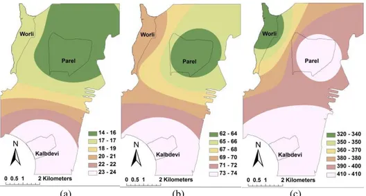
Figs. 7 (a), (b) and (c) are contour plots of average for SO2, NOx and SPM during post-monsoon months of the year. SO2 and NOx concentrations are as low as 7 and 51 μg/m3
in Parel. The highest concentrations of SO2 and NOx are in Kalbadevi at 14 and 71 μg/m
3
respectively. SPM concentration is high in Parel at
343 μg/m3 and low in Worli at 269 μg/m3
, though both are higher than the standard limit. Here too, it may be observed that pollutants SO2 and NOx may be transported from Kalbadevi to Worli to Parel, but SPM may be transported in the opposite direction.
Contour plots for winter season are shown in Figs. 8 (a), (b) and (c). SO2 and NOx are low in Parel at 14 and 62 μg/m3
, respectively. Kalbadevi has a concentration as high as 24, 74 and 414 μg/m3
for SO2, NOx and SPM respectively. Remarkably, here SPM apparently followed the opposite low direction: from Kalbadevi and Parel to Worli. The concentration of SPM in Worli was 323 μg/m3
, which is low. Here, too, pollutants SO2 and NOx had the same spatial pattern of being transported from Kalbadevi to Worli to Parel but SPM may go from Kalbadevi and Parel to Worli.
(a) (b) (c)
Figure 5. Annual average concentration (μg/m3
) of (a) SO2, (b) NOx and (c) SPM
(a) (b) (c)
Figure 6. Monsoon (June, July, August and September) concentrations (μg/m3
146 Figs. 9 (a), (b) and (c) show contour plots for the pre-monsoon season. Here, the spatial pattern of SO2, NOx and SPM concentrations do not match. For SO2, Parel and Kalbadevi display fairly low concentrations (8 μg/m3
) which are comparable to the values observed in Worli (9 μg/m3
). For NOx, Worli and Kalbadevi have the same concentration at 36 μg/m3
, which is maximum. For SPM, Parel showed higher concentration (296 μg/m3) than Worli (231 μg/m3
). For the entire region, SPM concentration was higher than the permissible limit, except during the monsoon season.
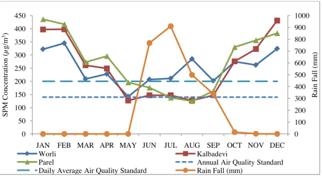
The average wind speed and maximum temperature of every month has been represented in Fig. 10. The maximum wind speed is in the monsoon season, leading to low concentration level of pollutants. The temperature was high and wind speed was low in
October, November and December. Fig. 11 shows SPM concentration in terms of monthly average. SPM concentration is low from May to September, which corresponds to the monsoon season in the study area. National Ambient Air Quality Standard (NAAQS; CPCB, 2008) prescribes annual and daily air quality standard 140 and 200 μg/m3
, respectively for SPM but the measured values were higher than that except during the monsoon season at all locations. The concentration is low during the monsoon season and high during the remaining seasons due to precipitation. Rainfall is high from June to September peaking in July, as shown in Fig. 11. The high rainfall washout the pollutants and show lower pollution levels in that period. Temperature, wind speed and rainfall data was collected from Indian Meteorological Department, Mumbai.
(a) (b) (c)
(a) (b) (c)
Figure 7. Post-monsoon (October and November) concentration (μg/m3
) of (a) SO2, (b) NOx and (c) SPM
Figure 8. Winter (December and January) concentration (μg/m3
147
5. Conclusions
Interpolation technique of ArcGIS was used for air pollutants such as SO2, NOx and SPM for Mumbai region. Inverse Distance Weighting (IDW) tool of ArcGIS was used for air quality assessment with a view to understand the variability of air pollutant concentrations across the city. The analyses have been performed for four distinct seasons: winter, pre-monsoon, monsoon and post-monsoon. The city experiences distinct drop in air pollution during rainy season (monsoon), which spans over four months (June-September). The spatial pattern of annual average, winter and post-monsoon seasons displayed
similar pattern for SO2 and NOx. The pre-monsoon and post-monsoon seasons showed a similar pattern for SPM. Except these, all showed different patterns for pollutant over the region. All three pollutants showed different patterns in pre-monsoon and monsoon. IDW technique appears to be an appropriate navigation tool for analysis of spatial variation of air quality. It does not require meteorological and emission data, with monitored concentration of pollutants being the only dataset needed. Monitoring data is easy and economical to obtain while collection of emission and meteorological data needs more resources in terms of time and costs.
0 2 4 6 8 10 12 14 16 18
25 27 29 31 33 35 37
JAN FEB MAR APR MAY JUN JUL AUG SEP OCT NOV DEC
W
ind Spe
ed
(k
ph)
T
em
p
era
tu
re (
o
C
)
Month
Temperature (oC) Wind Speed (kph)
AN B AR R AY UN UL G P CT NOV C
)
rli evi
arel rd
rd )
Figure 10. Monthly maximum temperature and average wind speed
AN B AR R AY UN UL G P CT NOV C
)
rli evi
arel rd
rd )
(a) (b) (c)
Figure 9. Pre-monsoon (February, March, April and May) concentration (μg/m3
148 However, this study has some limitations. For instance, air quality data was available only at three monitoring sites over the entire region and measurement on meteorological parameters was not available at sites. Enhanced air quality monitoring network and inclusion of meteorological parameters will help understand the atmospheric transportation of pollutants, leading to rigorous spatial interpolation and prediction.
References
Alcamo J, Mayerhofer P, Guardans R, van Harmelen T, van Minnen J, Onigkeit J, Posch M, de Vries B. An integrated assessment of regional air pollution and climate change in Europe : findings of the AIR-CLIM Project. Environmental Science and Policy 2002; 5(4): 257-72. Bollen J, Hers S, van der Zwaan B. An integrated
assessment of climate change, air pollution, and energy security policy. Energy Policy 2010; 38(8): 4021-30. Bollen J, van der Zwaan B, Brink C, Eerens H. Local air
pollution and global climate change: A combined cost-beneit analysis. Resource and Energy Economics 2009; 31(3): 161-81.
Candiani G, Carnevale C, Finzi G, Pisoni E, Volta M. A comparison of reanalysis techniques: applying optimal interpolation and Ensemble Kalman Filtering to improve air quality monitoring at mesoscale. Science of the Total Environment 2013; 458-460: 7-14. Census. Census of India Organization [homepage on the
Internet]. Ministry of Home Affairs, Government of India. 2011. Available from: http://www.censusindia. gov.in/Central Pollution Control Board (CPCB). National Ambient Air Quality Monitoring 2008. 2008.
Cinderby S, Forrester J. 2005. Facilitating the local governance of air pollution using GIS for participation. Applied Geography 2005; 25(2): 143-58.
Contini D, Donateo A, Elefante C, Grasso FM. Analysis of particles and carbon dioxide concentrations and luxes in an urban area : Correlation with trafic rate and local micrometeorology. Atmospheric Environment 2012; 46, 25-35.
Duh JD, Shandas V, Chang H, George LA. Rates of urbanisation and the resiliency of air and water quality. Science of the Total Environment 2008; 400(1-3): 238-56.
Gulia S, Shrivastava A, Nema AK, Khare M. Assessment of urban air quality around a heritage site using AERMOD: a case study of Amritsar city, India. Environmental Modeling and Assessment 2015; 20(6): 599-608. doi: 10.1007/s10666-015-9446-6
Gulliver J, Briggs D. STEMS-Air: A simple GIS-based air pollution dispersion model for city-wide exposure assessment. Science of the Total Environment 2011; 409(12): 2419-29.
Huff G, Angeles L. Globalization, industrialization and urbanization in Pre-World War II Southeast Asia. Explorations in Economic History 2011; 48(1): 20-36. Janssen S, Dumont G, Fierens F, Mensink C. Spatial
interpolation of air pollution measurements using CORINE land cover data. Atmospheric Environment 2008; 42(20): 4884-903.
Järvi L, Rannik Ü, Mammarella I, Sogachev, Aalto PP, Keronen P, Siivola E, Kulmala M, Vesala T. Annual particle lux observations over a heterogeneous urban area. Atmospheric Chemistry and Physics 2009; 9: 7847-56. doi: 10.5194/acp-9-7847-2009
0 100 200 300 400 500 600 700 800 900 1000 0 50 100 150 200 250 300 350 400 450
JAN FEB MAR APR MAY JUN JUL AUG SEP OCT NOV DEC
R ain F all (m m ) S P M C o n cen tr at io n ( µg /m 3) Worli Kalbadevi
Parel Annual Air Quality Standard
Daily Average Air Quality Standard Rain Fall (mm)
Figure 11. SPM concentrations (average of each month) for three locations of Mumbai compared with annual and daily air quality standard (140 and 200 μg/m3
149
Sohrabinia M, Khorshiddoust AM. Application of satellite data and GIS in studying air pollutants in Tehran. Habitat International 2007; 31(2): 268-75.
van Loon M. Testing interpolation and iltering techniques in connection with a semi-Lagrangian method. Atmospheric Environment. Part A. General Topics 1993; 27(15): 2351-64.
Vienneau D, de Hoogh K, Briggs D. A GIS-based method for modelling air pollution exposures across Europe. Science of the Total Environment 2009; 408(2): 255-66. Wang YQ, Zhang XY, Draxler RR. TrajStat: GIS-based
software that uses various trajectory statistical analysis methods to identify potential sources from l o n g - t e r m a i r p o l l u t i o n m e a s u r e m e n t d a t a . Environmental Modelling and Software 2009; 24(8): 938-39.
Wong DW, Yuan L, Perlin SA. Comparison of spatial interpolation methods for the estimation of air quality data. Journal of Exposure Analysis and Environmental Epidemiology 2004; 14(5): 404-15. doi: 10.1038 sj.jea.7500338
Yennawar PK. Air pollution measurement system in India. Studies in Environmental Science 1978; 2: 91-93. Zhang Q, Wei Y, Tian W, Yang K. GIS-based emission
inventories of urban scale: a case study of Hangzhou, China. Atmospheric Environment 2008; 42(20): 5150- 65.
Received 10 May 2016 Accepted 6 June 2016
Correspondence to
Dr.Awkash Kumar
Centre for Environmental Science and Engineering, Indian Institute of Technology Bombay,
Mumbai -400 076, India
E-mail: [email protected]; [email protected] Jensen SS, Berkowicz R, Hansen HS, Hertel O. A danish
decision-support GIS tool for management of urban air quality and human exposures. Transportation Research Part D: Transport and Environment 2001; 6(4): 229-41.
Jha DK, Sabesan M, Das A, Vinithkumar NV, Kirubagaran R. Evaluation of interpolation technique for air quality parameters in Port Blair, India. Universal Journal of Environmental Research and Technology 2011; 1(3): 301-10.
Kan H, Chen R, Tong S. Ambient air pollution, climate change, and population health in China. Environmental International 2012; 42: 10-19.
Kanada M, Fujita T, Fujii M, Ohnishi S. The long-term impacts of air pollution control policy : historical links between municipal actions and industrial energy efficiency in Kawasaki City, Japan. Journal of Cleaner Production 2013; 58: 92-101.
Ketzel M, Berkowics R, Hvidberg M, Jensen SS, Raaschou-Nielsen O. Evaluation of AirGIS : a GIS- based air pollution and human exposure modelling system. International Journal of Environment and Pollution 2011; 47: 226-38. doi: 10.1504/IJEP.2011. 047337
Kim S. Industrialization and urbanization: did the steam engine contribute to the growth of cities in the United States?. Explorations in Economic History 2005; 42(4): 586-98.
Kumar A, Dikshit AK, Fatima S, Patil RS. Application of WRF model for vehicular pollution modelling using AERMOD. Atmospheric and Climate Sciences 2015; 5(2): 57-62. doi: 10.4236/acs.2015.52004
Kumar A, Gupta I, Brandt J, Kumar R, Dikshit AK, Patil RS. Air quality mapping using GIS and economic evaluation of health impact for Mumbai city, India. Journal of the Air and Waste Management Association 2016; 66(5): 470-81.
Li C, Hsu NC, Tsay SC. A study on the potential applications of satellite data in air quality monitoring and forecasting. Atmospheric Environment 2011; 45(22): 3663-75.
Maantay J. Asthma and air pollution in the Bronx: methodological and data considerations in using GIS for environmental justice and health research. Health and Place 2007; 13(1): 32-56.
Marquez LO, Smith NC. A framework for linking urban form and air quality. Environmental Modelling and Software 1999; 14(6): 541-48.
Nemitz E, Jimenez JL, Huffman JA, Ulbrich IM, Canagaratna MR, Worsnop DR, Guenther AB. An eddy-covariance system for the measurement of surface/atmosphere exchange fluxes of submicron aerosol chemical species-irst application above an urban area. Aerosol Science and Technology 2008; 42(8): 636-57. doi: 10. 1080/02786820802227352