Quantum Processes: A Novel Optimization for Quantum Simulation
∗A.K. MARON1,∗∗, R.H.S. REISER2, M.L. PILLA2 and A.C. YAMIN2
Received September 30, 2012 / Accepted September 9, 2013
ABSTRACT. The simulation of quantum algorithms in classical computers demands high processing and storing capabilities. However, optimizations to reduce temporal and spatial complexities are promising and capable of improving the overall performance of simulators. The main contribution of this work con-sists in designing optimizations to describe quantum transformations using Quantum Processes and Partial Quantum Processes, as conceived in the qGM theoretical model. These processes, when computed on the VPE-qGM execution environment, reduce the execution time of the simulation. The performance evaluation of this proposal was carried out by benchmarks that include sequential simulation of quantum algorithms up to 24 qubits and instances of Grover’s Algorithm. The results show improvements in the simulation of general, controled transformations since their execution time was significantly low, even for systems with several qubits. Furthermore, a solution based on GPU computing for dealing with transformations that still have a high simulation cost in the VPE-qGM is also discussed.
Keywords:Quantum Simulation, VPE-qGM, Quantum Processes.
1 INTRODUCTION
Quantum Computing (QC) predicts the development of quantum algorithms that, in various sce-narios, are much faster than their classical versions [1, 2]. However, such algorithms can only be efficiently executed on quantum computers, which are currently unavailable for general purpose use. In this context, quantum simulation softwares, such as [3, 4, 5, 6] and [7], were proposed so researchers can anticipate the behaviors of the algorithms when executed on quantum hardware. Despite all the work already done, several approaches for simulation can still be explored.
The VPE-qGM (Visual Programming Environment for the Quantum Geometric Machine Model) [8] is a quantum simulator under development including both characterizations, visual
∗Work presented in the XXXIV Congresso Nacional de Matem´atica Aplicada e Computacional. ∗∗Corresponding author: Adriano K. Maron
1Graduate Program in Computer Science, University of Pittsburgh, Pittsburgh PA, USA. E-mail: [email protected] 2Graduate Program in Computer Science, PPGC/UFPEL, Technological Development Center, UFPel – Federal Univer-sity of Pelotas, 96010-610 Pelotas, RS, Brazil.
modeling, and distributed simulation of quantum algorithms, showing the application and evo-lution of quantum computing through integrated graphical interfaces. The current focus of this project is related to the exponential growth in the matrices associated to multi-qubit transforma-tions, where the efforts are towards the reduction of the temporal complexities associated to the execution of a muti-qubit quantum transformation.
In this context, the main contribution of this work is theextension of theVPE-qGM simula-tion capabilities through the implementasimula-tion of two concepts: Quantum Process (Q P) and Quantum Partial Process (Q P P). According to the specifications of theqGMmodel, these new concepts can be explored for modeling quantum transformations and reducing the compu-tations in a simulation. They are the mathematical structure underling the modeling of quantum parallelism in massive parallel architectures, such as GPUs (Graphic Processing Units), as de-scribed in [9].
This article is structured as follows: Section 2 comprehends the conceptual background related to this work. The theory and implementation regarding theQPsandQPPsare presented in Sec-tion 3. SecSec-tion 4 contains the performance analysis of the simulaSec-tion ofQPsandQPPs. Discus-sions concerning the results and main contributions of this work are presented in Section 5.
2 PRELIMINARY
Some concepts of QC are necessary to understand the contribution proposed in this work. Thus, an introduction of quantum computing and the qGM (Quantum Geometric Machine) model [10] are presented in the following subsections.
2.1 Quantum Computing
InQC, the qubit is the basic information unit, being the simplest quantum system, defined by a unitary and bi-dimensional state vector. Qubits are generally described in Dirac’s notation [11], by|ψ =α|0 +β|1. The coefficientsαandβare complex numbers for the amplitudes of the corresponding states in the computational basis (space states). These coefficients must respect the condition|α|2+ |β|2=1, which guarantees the unitarity of the state vector of the quantum system represented by(α, β)t.
The state space of a quantum system with multiplequbitsis obtained by the tensor product of the space states of its subsystems. Considering a quantum system with twoqubits,|ψ =α|0+β|1 and|ϕ =γ|0 +δ|1, the state space comprehends the tensor product|ψ ⊗ |ϕ, described by α·γ|00 +α·δ|01 +β·γ|10 +β·δ|11.
Transition states in aN-dimensional quantum system is performed by unitary quantum transfor-mations, defined by square matrices of orderN(2Ncomponents sinceN is the number ofqubits
in the system). The matrix notation ofHadamardand its application over a one-qubit system are, respectively, given as
H = √1
2
1 1
1 −1
and H|ψ = √1 2
1 1
1 −1
×
α β
=√1
2
α+β α−β
Quantum transformations simultaneously applied to differentqubitsare obtained by the applica-tion of the tensor product between the corresponding matrices, as in the following example:
H⊗2= √1
2
1 1
1 −1
⊗√1
2
1 1
1 −1
=1
2
⎛
⎜ ⎜ ⎜ ⎝
1 1 1 1
1 −1 1 −1
1 1 −1 −1
1 −1 −1 1
⎞
⎟ ⎟ ⎟ ⎠
. (2.2)
Besides the multi-dimensional transformations obtained by the tensor product, controlled transformations can also be used in quantum systems. TheCNOTtransformation acts over two qubits|ψand|ϕ, applying the NOT (Pauli X) transformation to one of them (target qubit), considering the current state of the other (control). Figure 1(a) shows the matrix notation of the
CNOTtransformation and its application to a generic two-qubit quantum state. The correspond-ing representation (quantum gate) in the quantum circuit model is presented in Figure 1(b).
(a) Evolution of quantum state (b) Quantum circuit
Figure 1: Representations of the CNOT gate.
By the composition and synchronization of quantum transformations, computations exploring the potentialities of quantum parallelism are created. However, the exponential increase of mem-ory usually arises in such computations. As a consequence, there is a loss of performance in the simulation of multidimensional quantum systems. Therefore, optimizations for efficient repre-sentation of multi-qubit quantum transformations are necessary.
2.2 qGM Model
TheqGMmodel follows the concepts of the domain theory closely related to the Girard’s coher-ent spaces [12]. The objects of the processes domainD∞, as introduced in [13] and [14], define coherent sets which provide interpretation for possibly infinite quantum processes. The processes and states are labeled by points in a geometric space, which characterizes the computational basis as ann-dimensional subspace of the Hilbert (H) space.
of the computational basis, stores α√+β
2 . Similarly, the second memory position, labeled as|1,
receives the α√−β
2 amplitude. Such execution is performed accordingly to the behavior of the
transformation, simulating the evolution of the quantum system.
The interpretation ofQPPsis obtained from the partial application of a quantum gate due to the existence of uncertainties related to some sets of vectors.
Consider the gateH⊗2defined in (2.2). Each single subset in this construction interprets aQ P P
corresponding to a matrix with only one defined line, and all the others being unknown (in-dicated by the bottom element ⊥). Considering as context the elements of the computational basis(|00,|01,|10,|11), it is possible to obtain the final global state|1by the union
(inter-preting the amalgamated sum on the process domain ofqGMmodel) of states. By this statement, it is possible to define partial states as in the following matrix-notation:
|0.1x⊥=H⊥⊗H|0 = ⎛ ⎝ 1 √ 2 1 √ 2 ⊥ ⊥ ⎞ ⎠⊗ ⎛ ⎝ 1 √ 2 1 √ 2 1 √ 2 −1 √ 2 ⎞ ⎠ ⎛ ⎜ ⎜ ⎜ ⎝ 0 1 0 0 ⎞ ⎟ ⎟ ⎟ ⎠ = ⎛ ⎜ ⎜ ⎜ ⎜ ⎝ 1 2 −1 2 ⊥ ⊥ ⎞ ⎟ ⎟ ⎟ ⎟ ⎠
|1.1x⊥=H⊥⊗H|0 = ⎛ ⎝ ⊥ ⊥ 1 √ 2 −1 √ 2 ⎞ ⎠⊗ ⎛ ⎝ 1 √ 2 1 √ 2 1 √ 2 −1 √ 2 ⎞ ⎠ ⎛ ⎜ ⎜ ⎜ ⎝ 0 1 0 0 ⎞ ⎟ ⎟ ⎟ ⎠ = ⎛ ⎜ ⎜ ⎜ ⎜ ⎝ ⊥ ⊥ 1 2 −1 2 ⎞ ⎟ ⎟ ⎟ ⎟ ⎠
Both states|0.1x⊥and|1.1x⊥are approximations of|1 = √12(1,−1,1,−1)t.
Although it is not the focus of this work, theqGMmodel provides interpretation for other quan-tum transformations, such as projections for measure operations.
3 QPPS: A PROPOSAL FOR OPTIMIZATION OF QUANTUM SIMULATION IN THE VPE-QGM
The VPE-qGM environment is being developed aiming at the support for modeling and dis-tributed simulation of algorithms fromQC, considering abstraction of theqGMmodel. By fol-lowing such abstractions, the concept of Quantum Process was implemented in the execution library of theVPE-qGM, calledqGM-Analyzer.
The main extensions consider the representation of controlled and non-controlled transforma-tions, and related possible synchronization. The specifications of these and other new features are described in the following subsections.
3.1 Non-Controlled Quantum Gates
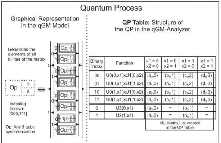
Figure 2: QP and its representation by applying EPs.
In Figure 2,MLstores the matrices associated with quantum transformations. Each line inML
is generated by functions, which are indicated in the second column of the Q P T able. These functions (U0,U1 eU2) describe the corresponding quantum transformation of the application modeled in the VPE-qGM.
The tuples of each line are obtained by changing the values of the parametersx1 andx2. The first tuple corresponds to the value obtained by the scalar product between the corresponding functions. The second indicates the column in which the value will be stored.
The matrix-order inMLis defined from the number of functions (n) grouped together. In Fig-ure 2, the first matrix inML, indicated byM1, hasn =2. Similarly,M2hasn=1.
It is interesting that the order of each matrix inMLcan be arbitrarily determined. Although, there is an exponential growth in memory consumption. Hence, a balance between the order and the number of matrices inML(|M L|) interferes directly in the performance of an application. Besides the ML, it is necessary to create a list (see in (3.1)) containing auxiliary values for indexing the amplitudes of the state space, which must be multiplied by each value of the matrices inML. In such list,qindicates the total number of qubits in the quantum application.
sizes L ist =2q−n,2q−(2∗n), . . . ,2q−(|M L|∗n) (3.1)
Based on the concept of partial processes defined as partial objects in theqGM model, it is possible to split theQ P described in Figure 2 in twoQPPs. Figure 3 contains the description of the Q P P0, which is responsible for the computation of all new amplitudes of the states in
the subset of memory positionsMQ P P0 = {0,1,2,3}. Similarly, the Q P P1is responsible for
computing the amplitudes in the complement set ofMQ P P0, indicated asMQ P P1 = {4,5,6,7},
F
igure
3
:
P
os
si
bl
e
Q
PPs
for
a
3
qubi
t
g
at
The QPPs contribute with the possibility of establishing partial interpretations of a quantum transformation. ComplementaryQPPs(that interpret distinct line sets) can be synchronized and executed independently (in different processing nodes of a multiprocessor system). The bigger the number ofQPPssynchronized, the smaller is the computation executed by each one, result-ing in a low-cost of execution.
3.2 Definition of Controlled Quantum Gates
Fornon-controlledquantum gates, it is possible to model all the evolution of the global state of a quantum system witha singleQ P. However, this possibility can not be applied to controlled quantum gates.
The complete description of CNOT transformation is obtained through the expressions in Eq. (3.2), which defines a set ofQPPs, called QPP Set. QPPsfor theCNOT transformation have their structures illustrated in Figure 4. TheQ P P1, in Figure 4(a) and associated toE x p1,
describes the evolution of the states in which the state of the control qubit is|1(requiring the application of the PauliXtransformation to the target qubit). The evolution of the states in which the control qubit is|0is modeled byE x p2generating the Q P P2, illustrated in Figure 4(b). As
these states are not modified, the execution of theQ P P2is not mandatory.
E x p1=C(1),X E x p2=C(0),I d (3.2)
(a) Q P P1: change amplitudes (b) Q P P2: do not change amplitudes
Figure 4: QPPs for the modeling of the CNOT gate.
In general,|Q P P Set| = |E x p| = 2nC, where nC is the total number of control qubits in all gates applied. However, it is only necessary the creation/execution of theQPPsin a sub-set (QPP Subset) ofQPP Set. If only one controlled gate is applied,|Q P P Subset| =1. When
nCcontrolled qubits are considered in a synchronization of controlled gates,|Q P P Subset| =
2nC
−1.
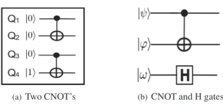
Now, consider the synchronization of CNOT transformation, as shown in Figure 5(a). By
VPE-qGM environment, this configuration is modeled using the expressions in (3.3). Hence, |Q P P Set| =4. However, theQ P P4, associated to the expressionE x p4, does not change any
amplitude and should not be created/executed.
E x p1 = C(1),X,C(1),X E x p2 = C(1),X,C(0),I d E x p3 = C(0),I d,C(1),X E x p4 = C(0),I d,C(0),I d
In a synchronization mixing controlled and non-controlled gates (different from Id), all the amplitudes are modified. Hence, Q P P Subset = Q P P Set. The configuration illustrated in the Figure 5(b) is modeled by the expressions in (3.4).
E x p1=C(1),X,H and E x p2=C(0),I d,H (3.4)
Thus, it means that twoQPPs, identified by Q P P1 and Q P P2, are associated to the
expres-sions in E x p1andE x p2, respectively. However, it is not possible to discard the execution of
the Q P P2, once it modifies the amplitudes of some states. Those changes are due to theH
transformation, which isalwaysapplied to the last qubit, despite the control state of theCNOT
transformation.
(a) Two CNOT’s (b)CNOT and H gates
Figure 5: Modeling synchronization of controlled gates.
3.3 Recursive Function
After building theQPPs, a recursive operator is applied to the matrices inMLfor computing the amplitudes of the new global state of the quantum system. This operator dynamically generates all values associated to the resulting matrix obtained by the tensor product of the transformations, defining the quantum application. Besides, a value indexing the amplitude is also generated. The algorithmic description of this procedure with some optimizations is shown in Figure 6.
The execution time of this algorithm grows exponentially when new qubits are added. When analyzing the use ofQPsandQPPsexclusively for the representation of quantum gates, there is a high-cost related to temporal complexity, specially whenHadamardgates are applied. Such cost reflects directly in the execution time. However, this approach presents a low-cost related to spatial complexity, once the matrices stored during the execution have maximum size of 32×32.
4 PERFORMANCE ANALYSIS OF THE OPTIMIZATIONS
For validation and performance analysis of the simulation withQPsandQPPs, the following three study-cases were considered:
C1: Reversible circuit benchmarks from [15];
C2: Hadamardgates up to 14 qubits;
ifmatr i x I nd ex=num Matr i ces−1then forl=0tosi ze(Matr i ces[matr i x I nd ex])do
r es←0;
li ne←Matr i ces[matr i x I nd ex][l][0]; li ne P os←Matr i ces[matr i x I nd ex][l][0]; forcolumn=0tosi ze(li ne)do
pos ←base P os+li ne[column][1];
r es←r es+(par ti alV alue×li ne[column][0] ×memor y[1][pos]);
end for
wr i te P os←mem P os+(li ne P os×si zes Li st[matr i x I nd ex]);
r es←r es+memor y[0][wr i te P os]; memor y[0][wr i te P os] ←r es; end for
else
forl=0tosi ze(Matr i ces[matr i x I nd ex])do li ne←Matr i ces[matr i x I nd ex][l][1]; li ne P os←Matr i ces[matr i x I nd ex][l][0]; forcolumn=0tosi ze(li ne)do
next base P os←base P os+(li ne[column][1] ×si zes Li st[matr i x I nd ex]);
next par ti alV alue←par ti alV alue×li ne[column][0]; Apply V alues(Matr i ces,num Matr i ces,si zes Li st,memor y,
next par ti alV alue,matr i x I nd ex+1,next base P os,
mem P os+(li ne P os×si zes Li st[matr i x I ndex]));
end for end for end if
Figure 6: Algorithm for the execution of the computations over QPs and QPPs.
The evaluation with benchmarks C1 and C2 considered 10 simulations for each study-case, and the average of execution time and memory consumption were measured. ForC3, only one execution of each instance of Grover’s algorithm was performed, however each step of the simulation was monitored and therefore several samples of the simulation time for each step were collected. From those, the average for the simulation time associated with each step was obtained. The hardware considered for each scenario is characterized as follows:
C1andC2: Core i5-2410M, 4 GB RAM, Python 2.7 and Ubuntu 11.10 64 bits;
C3: Core i7-3770, 8 GB RAM, Python 2.7 and Ubuntu 12.04 64 bits.
4.1 Reversible Circuits and Hadamard Gates
quan-tum algorithms usingEPs, considering the optimizations described in [16]. The main features of each algorithm and the results obtained are presented in Tables 1 and 2.
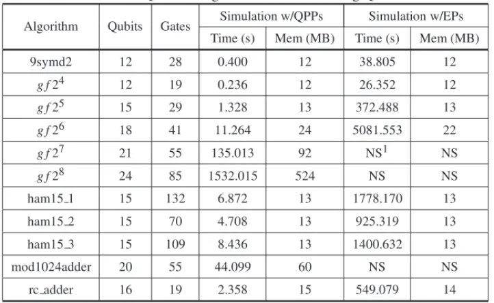
Table 1: Quantum algorithms simulated using QPPs.
Algorithm Qubits Gates Simulation w/QPPs Simulation w/EPs Time (s) Mem (MB) Time (s) Mem (MB)
9symd2 12 28 0.400 12 38.805 12
g f24 12 19 0.236 12 26.352 12
g f25 15 29 1.328 13 372.488 13
g f26 18 41 11.264 24 5081.553 22
g f27 21 55 135.013 92 NS1 NS
g f28 24 85 1532.015 524 NS NS
ham15 1 15 132 6.872 13 1778.170 13
ham15 2 15 70 4.708 13 925.319 13
ham15 3 15 109 8.436 13 1400.632 13
mod1024adder 20 55 44.099 60 NS NS
rc adder 16 19 2.358 15 549.079 14
NS: Not Supported. Simulation time over 4 hours.
Table 2: Quantum algorithms simulated using QPs.
Algorithm Qubits Gates Simulation w/QPs Simulation w/EPs Time (s) Mem (MB) Time (s) Mem (MB)
H⊗11 11 11 6.816 12 7.882 12
H⊗12 12 12 25.292 12 28.281 12
H⊗13 13 13 97.401 12 111.572 12
H⊗14 14 14 348.923 12 496.934 12
Quantum algorithms up to 24 qubits were simulated. The memory consumption was higher for the new proposal due to slightly more complex structures necessary to represent the new components. However, the trade off between memory usage and execution time is positive for the new approach.
As the optimizations regardingQPsandQPPsonly affect quantum gates, the high memory cost is due to the storage of the amplitudes of the quantum system. This structure limits theVPE-qGM
to the simulation of algorithms with approximately 25 qubits in a 4G B R AM machine. The improvement for controlled operations is due to the optimization focused on the identification of
Despite the different sizes of the state vectors forH⊗11, H⊗12, H⊗13and H⊗14, the memory usage remained the same (12 MB). This behavior is explained by the memory management of the Python interpreter. For all Python processes, an initial 12 MB memory space is allocated, even if the process execution requires less. As the data referred to memory usage presented in the Tables 1 and 2 was obtained using thetopsoftware, only the total amount of memory allocated to the process was exhibited instead of the actual space occupied by allocation calls. For algorithms with more than 12 qubits, which generate bigger state vectors, the Python interpreter dynamically allocates more memory when necessary.
4.2 Grover’s Algorithm Simulation
The simulation of the Grover’s algorithm follows the circuit described in [17]. Herein, the focus is in the simulation time since the memory consumption follows the values previously presented in Table 2.
Table 3 describes the number of iterations of the Grover’s (G) operator, the total number of simulation steps generated and the total simulation time. TheGoperator is comprised by:
• Uf: oracle that applies a controlled transformation to all qubits;
• 2|ψ ψ| −I: amplitude amplification operator with five steps as defined in [17].
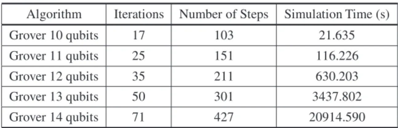
Table 3: Grover’s Algorithm Simulation.
Algorithm Iterations Number of Steps Simulation Time (s)
Grover 10 qubits 17 103 21.635
Grover 11 qubits 25 151 116.226
Grover 12 qubits 35 211 630.203
Grover 13 qubits 50 301 3437.802
Grover 14 qubits 71 427 20914.590
The highest standard deviation for these simulations was 0.29% of the average, measured for the
Grover 10 qubits. As it can be seen, due to the many steps necessary, the simulation time suffers an exponential increase when systems with more qubits are simulated.
Figure 7: Computation time required by each step of Grover’s algorithm
TheOracleis applied at each iteration ofG, but it does not significantly affect the total time due to partial execution withQPPs.
In particular, one can observe that:
(i) Steps from 1 to 5 refer to the amplitude amplification operator;
(ii) Steps 2 and 4 yield a more significant computation than controlled operators, since in the global context of the simulation they must be fully executed;
(iii) Step 3 is slightly more complex than theOracle, but as it is also described in terms of
QPPs, an efficient execution is obtained;
(iv) Steps 1 and 5 account for the greatest shares of the total simulation time. Being described by many Hadamard gates and executed at each iteration of theGoperator, they lead to a scenario where a transformation defined byH⊗13⊗I d is applied 854 times during the simulation (427 times for each step).
4.3 Related Work Results
The state-of-art in sequential simulation of quantum algorithms, characterized by the works of [7] and [6], represents the best performance reference for our work. As we do not have access to these simulators yet, simulations of these alternative software in our own hardware was not performed and therefore a direct performance comparison is not possible. However, it is possible to perform an approximated performance comparison of theVPE-qGM with the
QuIDDProsimulator according to the results presented in [7]. The simulated circuits include the following: ham15 1,ham15 2,ham15 3,rc adder, and 9s ymd2. It is important to note that those results were obtained using a different hardware configuration (Athlon 1.2 GHz processor with 1GB of RAM).
• The former is related to Python language, which is interpreted and, consequently, slower than C, used in theQuIDDPro;
• The latter consists in the absence of optimizations for the storage of the state space in the
VPE-qGM, which is responsible for the high memory usage.
The results presented in [6] included some stabilizer circuits and factorization algorithms, which yet are not fully supported in theVPE-qGM environment. Thus, no comparison with PVLIB
was performed.
4.4 Expectations for GPU Computing
As discussed in Section 4.2, the simulation time of Grover’s algorithm is highly affected by theHadamardgates applied during the amplitude amplification operator. As our solution does not consider gate-by-gate simulation, currently the problem of high computational cost is being treated by the highly parallel architecture of GPUs.
Our first results in this regard, presented in [9], comprehends the simulation ofHadamardgates up to 21 qubits. Since this implementation is in its initial stages, algorithms such as Grover are not supported yet. However, as its computational cost is directly affected by the Hadamard gates, it is possible to estimate how it should perform on the parallel simulation on the GPU.
Table 4 shows results from simulations of Hadamard gates using the Python sequential ap-proach, presented in this work, and a GPU simulation described in [9]. The speedups reflect the efficiency of the parallel simulation and provide an approximation of the simulation time for an instance of the Grover’s algorithm. As≈ 97% of the Grover’s simulation time is spent on execution of Hadamard gates, it is feasible to state that a similar speedup may be obtained in the Grover’s parallel simulation in the GPU.
Table 4: Simulations of Hadamard gates with sequential and parallel approaches.
Transformation Sequential (s) GPU (s) Speedup
H⊗10 1.142 0.001 1142
H⊗11 4.383 0.001 4383
H⊗12 17.402 0.008 2175
H⊗13 68.956 0.020 3447
H⊗14 285.241 0.085 3355
H⊗15 1140.114 0.299 3813
5 CONCLUSION
simulation of the algorithms, this environment supports the simulation of algorithms up to 24 qubits. This limit is established by the memory consumption due to the storage of the state vec-tor of the algorithm.
ForHadamard gates, the limitation is related to the exponential growth in the simulation time. In our current hardware, the limit forHadamardgates is appropriately 16 qubits. The simulation of controlled quantum transformations has the benefit of a reduced number of operations in order to simulate state evolution. Hence, such simulation up to 24 qubits is possible.
Considering the state-of-art in quantum simulation, even after the optimizations described in this work, the best simulators available still outperforms theVPE-qGM. However, new improve-ments can be developed in theVPE-qGMto handle memory consumption and execution time. By exploring the visual tools provided by theVPE-qGM and its integration with optimized li-braries, this environment becomes an intuitive platform for the development and study of quan-tum algorithms.
With the recent development ofGPUs, several research areas are working with massive amounts of data and dealing with heavy calculations. The exploration of this approach in benefit of QC
is a novel research field and by optimizing algorithms and the computing power ofGPUs, new breakthroughs can be achieved.
The contribution of this work is the first of three steps towards a solution for quantum simulation not yet consolidated: the use of HPC’s (High Performance Computing) resources, such asGPUs
and clusters, coupled with optimizations that are capable of exploring patterns and mathematical properties intrinsic to quantum computing. Steps two and three of our project are respectively comprised by:(i)support for GPU/cluster simulation; and(ii)optimizations for efficient repre-sentation/storage of the state vector.
ACKNOWLEDGMENTS
This work is supported by the Brazilian funding agencies CAPES, FAPERGS (PqG 06/2010, process number 11/1520-1), and by the CNPq/PRONEX/FAPERGS Green Grid project.
RESUMO.A simulac¸˜ao de algoritmos quˆanticos em computadores cl´assicos exige alta ca-pacidade de processamento e armazenamento. Entretanto, otimizac¸ ˜oes voltadas `a reduc¸˜ao
das complexidades espacial e temporal s˜ao promissoras e capazes de melhorar o desempenho dos simuladores. A principal contribuic¸˜ao deste trabalho consiste no desenvolvimento de
otimizac¸ ˜oes para descric¸˜ao de transformac¸˜oes quˆanticas utilizando Processos Quˆanticos e
Processos Quˆanticos Parciais, seguindo as concepc¸˜oes do modelo te ´orico qGM. Esses pro-cessos, quando computados no ambiente de execuc¸˜ao VPE-qGM, reduzem o tempo de
exe-cuc¸˜ao das simulac¸ ˜oes. A avaliac¸˜ao de performance desta proposta foi efetuada utilizando
benchmarks que incluem a simulac¸˜ao sequencial de algoritmos quˆanticos com at´e 24 qubits e instˆancias do Algoritmo de Grover. Os resultados mostram uma melhora na simulac¸˜ao de
foram significantemente reduzidos, mesmo quando utilizados sistemas com muitos qubits.
Ainda, uma soluc¸˜ao baseada em GPUs voltada `a transformac¸ ˜oes que ainda possuem alto custo de simulac¸˜ao no VPE-qGM ´e discutida.
Palavras-chave:Simulac¸˜ao Quˆantica, VPE-qGM, Processos Quˆanticos.
REFERENCES
[1] L. Grover. “A fast quantum mechanical algorithm for database search”,Proceedings of the Twenty-Eighth Annual ACM Symposium on Theory of Computing, pp. 212–219, 1996, available at
<http://doi.acm.org/10.1145/237814.237866>(dec.2011).
[2] P. Shor. “Polynomial-time algoritms for prime factorization and discrete logarithms on a quantum computer”.SIAM Journal on Computing(1997).
[3] J. Agudelo & W. Carnielli. “Paraconsistent machines and their relation to quantum computing”. J. Log. Comput.,20(2) (2010), 573–595.
[4] A. Barbosa. “Um simulador simb´olico de circuitos quˆanticos”. Master’s thesis, Universidade Federal de Campina Grande (2007).
[5] H. Watanabe. “Qcad: Gui environment for quantum computer simulator”, 2002, available at
<http://apollon.cc.u-tokyo.ac.jp/watanabe/qcad/>(dec.2011).
[6] V. Samoladas. “Improved bdd algorithms for the simulation of quantum circuits”, inAnnual European Symposium on Algorithms. Berlin, Heidelberg: Springer-Verlag, (2008), 720–731.
[7] G. Viamontes. “Efficient quantum circuit simulation”. Phd Thesis, The University of Michigan, (2007).
[8] A. Maron, A. Pinheiro, R. Reiser & M. Pilla. “Consolidando uma infraestrutura para simulac¸˜ao quˆantica distribu´ıda”, inAnais da ERAD 2011. SBC/Instituto de Inform´atica UFRGS, (2011), 213– 216.
[9] A. Maron, R.H.S. Reiser & M.L. Pilla. “High-performance quantum computing simulation for the quantum geometric machine model”, inCCGRID 2013 IEEE/ACM International Symposium on Clus-ter, Cloud and Grid Computing. NY: IEEE Conference Publishing Services, May 2013, pp. 1–8.
[10] R. Reiser & R. Amaral. “The quantum states space in the qgm model”, inAnais/III WECIQ. Petr´o-polis/RJ: Editora do LNCC, (2010), 92–101.
[11] M.A. Nielsen & I.L. Chuang.Computac¸˜ao Quˆantica e Informac¸˜ao Quˆantica. Bookman (2003).
[12] J.-Y. Girard. “Between logic and quantic: a tract”, inLinear logic in computer science, P.R. Thomas Ehrhard, Jean-Yves Girard and P. Scott, Eds. Cambridge University Press, 2004, pp. 466–471. [On-line]. Available: http://iml.univ-mrs.fr/∼girard/Articles.html
[13] R. Reiser, R. Amaral & A. Costa. “Quantum computing: Computation in coherence spaces”, in Pro-ceedings of WECIQ 2007. UFCG – Universidade Federal de Campina Grande, (2007), 1–10.
[14] R. Reiser, R. Amaral & A. Costa. “Leading to quantum semantic interpretations based on coherence spaces”, inNaNoBio 2007. Lab. de II – ICA/DDE – PUC-RJ, (2007), 1–6.
[15] G.D.D. Maslov & N. Scott. “Reversible logic synthesis benchmarks page”, 2011, available at
[16] A. Maron, A. ´Avila, R. Reiser & M. Pilla. “Introduzindo uma nova abordagem para simulac¸˜ao quˆantica com baixa complexidade espacial”, inAnais do DINCON 2011. SBMAC, (2011), 1–6.
[17] A. Prokopenya. “Wolfram demonstrations project – quantum circuit implementing grover’s search algorithm”, 2009, http://demonstrations.wolfram.com/QuantumCircuitImplementingGroversSearch


![Table 4 shows results from simulations of Hadamard gates using the Python sequential ap- ap-proach, presented in this work, and a GPU simulation described in [9]](https://thumb-eu.123doks.com/thumbv2/123dok_br/18983701.458028/13.1063.315.813.977.1219/results-simulations-hadamard-python-sequential-presented-simulation-described.webp)
