Braz. J. Phys. vol.35 número1

Numerical Prediction of Nonequilibrium Hypersonic Flow

Around Brazilian Satellite SARA

Ghislain Tchuen,

Institut Universitaire de Technologie Fotso Victor

Universit´e de Dschang, BP. 134 Bandjoun - Cameroun

Yves Burtschell, and David E. Zeitoun

Technopole de Chateau Gombert, 13453 Marseille Cedex 13, France

Received on 29 June, 2004. Revised version received on 15 October, 2004

Hypersonic flows past Brazilian satellite SARA at zero angle of attack in chemical and thermal nonequilib-rium are investigated using an axisymmetric Navier-Stokes solver. The numerical solutions were carried out for freestream conditions equivalent to a typically re-entry trajectory with a range of Mach numbers from 10 to 25. The gas was chemically composed by seven air speciesO, N, N O, O2,N2, N O+, e

−

with 24 steps chemical reactions scheme and thermically characterized by a multi-temperature model. Comparisons have been made between the present computation and the distribution of pressure coefficient and the heat transfer obtained recently with Direct Simulation Monte Carlo Method[1]. The study also points out the influence of nonequilibrium phenomena like ionization, vibrational and electronic excitation on aerothermodynamic flow parameters.

1

Introduction

Recently, Sharipov predicted by the DSMC method and for a frozen flow (without chemical reactions), the aerothermo-dynamic parameters which are necessary for the calculation of the ballistic trajectory of re-entry and for the creation of an adequate aerothermic protection of a small reusable bal-listic Brazilian satellite SARA[1]. The atmospheric condi-tions used goes from the free molecular regime up to the hydrodynamic medium.

The development of the satellite re-entry into at-mosphere requires accurate prediction of the thermal pro-tection system for extremely high temperature. The vehicle flying with hypersonic velocity through the Earth’s upper atmosphere. This creates a detached shock wave around the vehicle and the kinetic energy is transformed into the inter-nal energy. Therefore, the shock layer is the site of inten-sive physico-chemical nonequilibrium processes such as vi-brational excitation, dissociation- recombination, electronic excitation, significant ionization and radiative heating[2]. These are commonly referred as high-temperature effects which causes considerable difficulties for accurate numer-ical and experimental simulations of the flowfield. Success-ful conception of such high technology would be obtained after some knowledge of the thermochemical nonequilib-rium phenomena and how they affect the performance of the vehicle.

In this study, an effort is being spent to the

numeri-cal prediction of the aerothermodynamic characteristics of satellite for very high altitude with a Knudsen number rel-atively suitable to the application of Navier-Stokes equa-tions. According to the Mach number and heating effects observed, nonequilibrium chemical, vibrational and elec-tronic modes are taken into account. The series of calcu-lations are carried out taking into account, in a progressive way the assumptions which allow as well as possible to ap-proach the reality of physics within the flow. The numerical simulations begin with a frozen air flow, followed by the taking into account of a chemical kinetics with 5 species in which the various couplings are included. The last step is made by an extension for conditions being able to cause sig-nificant ionization of gas (chemical kinetics with 7 species) and the electronic excitation of the species. An efficient and robust thermochemical nonequilibrium Navier-Stokes code based on Upwing technology with Riemann’s solver has been developed.

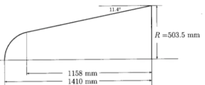
Figure 1. Shape of satellite SARA

2

Governing equations

The governing equations for a real gas are reported follow-ing the simplifications discussed by Lee[3]. The full laminar

Navier-Stokes equations for two-dimensional conservation equations are written as:

The mass conservation equation for each species,s,

∂ρs

∂t +

∂ρsuj

∂xj

+∂ρsV

j s

∂xj

=ωs (1)

The momentum conservation equation inxandydirections,

∂ρui

∂t +

∂(ρuiuj+pδij)

∂xj

+∂τij

∂xj

= 0 (2)

The total energy equation,

⌋

∂ρe

∂t +

∂((ρe+p)uj)

∂xj

+∂uiτij+qtj +qvmj+qej +

ns

s (ρshsVsj)

∂xj

= 0 (3)

The conservation equation of vibrational energy for each nonequilibrium molecule,

∂ρevm

∂t +

∂(ρevmuj) ∂xj

+∂(qvj+ρmevmV

j m)

∂xj

=QT−vm+Qvm−vr+Qvm−e (4)

The electron-electronic energy conservation equation

∂ρee

∂t +

∂((ρee+pe)uj)

∂xj

+∂(qej+

sρseesV

j s)

∂xj

=uj

∂pe

∂xj

−Qvm−e (5) +QT−e+Qel

In these equations, the electric field due to the presence of electrons in flow is expressed as:

− →

E ≃ − 1

Neǫ

− →

∇pe (6)

The shear stresses are modelled using the hypothesis of a newtonian fluid as:

τij =−µ

∂ui

∂xj

+∂uj

xi

−λ∂uk ∂xk

δij, with λ=−2

3µ (7)

⌈

The dynamic vicosityµsof each species is given by

Blot-tner et al.[4] and the thermal conductivity of each species is derived from Eucken’s[5]. The total viscosity and conduc-tivity of the gas are calculated using Wilke’s semi-empirical mixing rule[6].

The mass diffusion fluxes for s-species are given by Fick’s law with a single diffusion coefficientDsas:

ρsVsj =−ρDs

∂Ys

∂xj

(8) Where the expression of diffusion coefficient is obtained by assuming a constant Lewis number (Le=1.2). When

ion-ized species are included, the diffusion of ions and elec-trons is modeled with ambipolar diffusion as recommended

in ref[7]. The heat flux (conductive, chemical, vibrational and electronic counterparts) are defined as:

− →

Q =−→qtr+−→qv+−→qel+−→qchem (9)

with

− →_q

tr=−λtr∇T −→qv=

m=mol

−λv,m∇Tvm

− →_q

el=−λel∇Te −→qchem=

i

hiρsVsj (10)

ρe=

s=e

ρsCv,trs T+

1 2

s

ρsu2s

+

N M

m=1

ρmevm+ρee+

N S

s=1

ρsh0s (11)

is splitted between the translational-rotational, kinetic, vi-brational, electron-electronic contributions, and the latent chemical energy of the species. The total pressure is given by Dalton’s law as the sum of partial pressure of each species regarded as perfect gas.

p=

N S

s=1

ps=

s=e

ρsRsT+ρeReTe (12)

3

Numerical simulations

The governing equations are integrated using an efficient and robust thermochemical nonequilibrium Navier-Stokes solver. The present code is based on the Upwing technology with exact Riemann’s solver algorithm, in conjunction with a second-order MUSCL -TVD type scheme approach[8], coupled with a multi-block finite volume scheme.

The system of equations (1)-(5) can be reduced in only one as follows:

∂U

∂t +

∂(Fc+Fv)

∂xj

= Ω (13)

Where U is the conservative vector, Fc the convectif flux,

Fvthe viscous flux andΩthe source term.

The explicit formulation which gives the variation of

Ui,jduring time∆ton each cell(i, j)can be written in two

dimensional axisymmetric coordinate as[9]: ∆Ui,j

∆t +

1

Ai,jrαi,j

4

k=1

FkNk =αHi,j+ Ωi,j (14)

whereα = 1 for an axisymmetry coordinate system, and

α= 0for planar two-dimensions. This equation allows us to calculate numerically the all unknown variables in all com-putational domain. The exact Riemann solver and the Mim-mod limiter function are used for the convective fluxes. The viscous terms are classically discretized by second-order central difference approximation. The source termsΩare treated implicitly to relax the stiffness. The semi-implicit predictor-corrector schema can be written as:

⌋

P red.:

I−∆t

2

∂Ωi,j

∂Ui,j

∆Ui,j=−

∆t

2 .R

n_{; ∆U}

i,j =Un

+1/2

i,j −U n

i,j (15)

Corr.:

I−∆t∂Ωi,j ∂Ui,j

∆Ui,j=−∆t.Rn+1/2; ∆Ui,j =Ui,jn+1−U n

i,j (16)

⌈

whereRn _{is the residual calculated explicitly at time step}

n. The steady state is obtained after convergence of the un-steady formulation of the discretized equations. The algo-rithm is second order accurate in space and time.

The modified speed of sound which takes into account the nonequilibrium electronic is implemented in the flux

splitting procedure as[10]:

c2 =γ

_p

ρ

+ (γ−1) _T

Te

−1 _p

e

ρ (17)

where classical frozen speed of sound is obtained when

T =Te.

TABLE 1. Upstream conditions for satellite SARA

Mach 10 10 20 25

Altitude, (Km) 80 75 80 80

U∞,(m/s) 2811.2 2816.45 5622.4 7028

P∞,(Pa) 0.8627 2.08393 0.8627 0.8627

T∞,( o_K)

196.65 196.65 196.65 196.65

Twall/T∞ 1 1 1 1

Re 2161.80 4000 4323.6019 5404.5024

Kn 6.87x10−3

3.7143x10−3

6.874x10−3

6.874x10−3

Grid IM 50 50 60 60

Grid JM 50 50 80 90

∆xmin(m) 2.5946x10−4

2.5946x10−4

1.0230x10−4

4.6709x10−5

∆ymin(m) 2.0522x10−3

2.0522x10−3

2.4606x10−4

4

Results and comparisons

The conditions of simulation are defined from the following parameters:

The Mach number is given as:

Ma=

U∞

c (18)

wherecis the speed of sound defined earlier The Reynolds number is given as:

Re=

RU∞ρ∞

µ (19)

where Ris the largest satellite radius as shown in Fig. 1. These two parameters allow to define the gas rarefaction which is characterized with the Knudsen number as[1]:

Kn=Ma

Re

γπ

2 (20)

The various aerothermodynamic parameters calculated along the wall in this paper are defined as follows:

Skin friction coefficient

Cf =

τw

1 2ρ∞U

2 ∞

(21)

Pressure coefficient

Cp=

P−P∞

1 2ρ∞U

2 ∞

(22) Wall heat transfer coefficient

Ch= 1 Qw

2ρ∞U 3 ∞

(23)

Upstream conditions

The upstream conditions are chosen in order to make com-parisons with Sharipov’s results given in ref.[1]. In this paper the results are presented for 3 values of the Reynolds number (0,1 ; 10 and 4000) and for Mach number (5, 10, 20). The conditions used in this work are gathered in the table 1, and are extract from the abacus of the standard atmosphere[11]. The altitude of 80 km is retained because of the Reynolds number is close to 4000.

Boundary conditions

The boundary conditions are imposed along the satellite. The wall temperature is selected equal to the temperature of the upstream flow from which the various characteristics are given in the table 1. The walls are supposed chemically noncatalytic, no-slip and no-temperature jump boundary conditions are used. The freestream is hypersonic and all flow variables are known. The outflow is supersonic and therefore the zero gradient exit condition is appropriate. The influence of the temperature of wall on the variables aerothermodynamics was studied by Sharipov[1] and is not included in this study.

X (m)

Y(

m

)

0 0.3 0.6 0.9 1.2 1.5

0.3 0.6 0.9 1.2

Figure 2. Numerical grid.

Figure 2 shows the geometry and grid used in the cal-culations. The grid point is densely distributed near the wall and near the shock standoff distance. The minimum grid spacing inxandy directions are respectively carried in the table 1. The time step is classically determined by explicit stability criteria and the Courant-Friedrichs-Lewy (CFL) number used in all computations varying from 0.01 to 0.4.

Results

Case Mach 10

Figure 3 represents the translational temperature iso-contours in the flow atRe = 4000. The maximum value

of the temperature ratio T /T∞ behind the shock wave is around 20 which is 30% weaker than the value predicted by Sharipov. The obtained temperature can cause only a very weak dissociation of the oxygen molecules. Conse-quently, chemical nonequilibrium is not taken into account in this case. The skin friction coefficientCf, the pressure

coefficientCpand the wall heat transfer coefficientCh are

represented in Figs. 4, 5 and 6 as a function of the angleθfor two Reynolds numbers (2161.8 and 4000). The Reynolds number has a significant influence on the peak ofCf. For

identical Mach numbers, the evolution ofCf strongly

de-pends on two parameters : the radius of the satellite and the Reynolds number. One can notice that the passage of the altitude 80 to 75 km, involves a decrease of the peak of about 41.93%. The results obtained forCpandChare

com-pared in Figs. 5 and 6 with those obtained with DSMC[1]. The influence of the Reynolds number is also pointed out with an increase of 35.4% ofChat the stagnation point. For

10

9 8

7

6

5

4

3 2

1

X (m)

Y(

m

)

0 0.1 0.2 0.3 0.4 0.5

0.1 0.2 0.3 0.4 0.5

Level T/T

10 20

9 18

8 16

7 14

6 12

5 10

4 8

3 6

2 4

1 2

∞

∆Τ/Τ

∞= 2 Frozen gas

Re = 4000

Figure 3. Isocontours of translational temperature; Mach 10.

θ

Cf

10 20 30 40 50 60 70 80 90

0 0.02 0.04 0.06 0.08 0.1 0.12 0.14

Re = 2161,8

Re = 4000

Figure 4. Friction Coefficient; Mach 10.

θ

Cp

10 20 30 40 50 60 70 80 90

0.5 1 1.5 2

Re = 2161,8

Re = 4000

Re = 4000 ( DSMC )

Figure 5. Comparison with the DSMC of the coefficientCp; Mach 10.

θ

10 20 30 40 50 60 70 80 90 0

0.05 0.1 0.15 0.2 0.25 0.3 0.35

Re = 2161,8

Re = 4000

Re = 4000 ( DSMC )

Ch

Figure 6. Comparison with the DSMC of the coefficientCh; Mach 10.

Case Mach 20

When the velocity of the vehicle increases, more ki-netic energy is absorbed by the initial air molecules and the nonequilibrium processes such as vibrational excitation, rapid dissociation- recombinaison take place in the shock layer. Consequently, the physico-chemical phenomena are simultaneously set up and are included here. To simu-late this case, the upstream air flow is considered with 2 species (23.30% of O2 and 76.69% of N2). Behind the shock wave, the Park’s chemical kinetics model[12] with 5 species O, N, N O, O2, N2 and 17 chemical reactions is used. O2andN2are each characterized by their proper vi-brational temperature whileN Ois assumed to be in thermo-dynamic equilibrium with the translational temperature[13]. The Coupling Vibration-Dissociation (CVD) is taken into account according to the Park’s model[12] with an aver-age two temperature assumption. The coupling Vibration-Vibration(V-V) is given by Candler[14]. The influence of coupling V-V on the thermodynamic parameters is pre-sented. A comparison with the DSMC results is also made.

The translational temperature isocontours are plotted in Fig. 7 for frozen flow. The maximum value of the ratio

3

2 1

4

5

6

7

8

1

0

9

X (m)

Y(

m

)

0 0.1 0.2 0.3 0.4 0.5 0.1

0.2 0.3 0.4 0.5

Level T/T

10 75

9 67.5

8 60

7 52.5

6 45

5 37.5

4 30

3 22.5

2 15

1 7.5

∆T/T =7.5

∞

∞

Frozen gas

Re = 4323.6

Figure 7. Isocontours of translational temperature; Mach 20.

1

1

2

3

4

5

7

8 9

2

3

4

5

6

7

8

6

Level P/P

10 500

9 450

8 400

7 350

6 300

5 250

4 200

3 150

2 100

1 50

∞

∆_{P/P∞= 50}

With CVD

With CVD and V-V

Figure 8. Influence of the coupling V-V on isopressions, Mach 20, Re= 4323.6

TABLE 2. Various positions of the shock; SARA Mach 20

Mach 20 Frozen with CVD with V-V

X(m) 0,0350 0,0250 0,0225

δ=X/R(%) 6,9513 4,9652 4,4687

The influence of the nonequilibrium phenomena on the detachment of shock on the stagnation line is presented in table 2. Frozen case corresponds to a calculation without chemical reactions. The temperatures along the stagnation line are drawn in Fig. 9. The nonequilibrium vibrational of the molecules O2andN2 leads to a distinct distribution of temperatures (TvO₂, TvN₂). This justifies the use of the

model with three temperatures in spite of the strong Mach number, contrary to the use of a single temperature of vi-bration proposed by certain authors [15, 16]. Near the wall where temperature is low, one can note the influence of the V-V coupling. The difference between vibrational temper-atures is more important without the V-V coupling, which leads to a transfer of a part ofO2 energy of vibration to-wardsN2, and confirms the tendency to bring closer the two temperatures of vibration. One notices an increase of the temperature TvN₂ behind the shock wave. The

trans-rotational temperatureTis about 13 000K behind the shock wave. This maximum is not sufficient to cause a signifi-cant ionization of gas under the upstream conditions used. Therefore, the ionization and electronic nonequilibrium are neglected.

X (m)

Temp

er

atu

res

,

[°K

]

-0.03 -0.02 -0.01 0 0

2000 4000 6000 8000 10000 12000 14000

T Tv Tv

O2 N2

with V-V without V-V

Figure 9. Temperatures distribution along the stagnation line, Mach 20,Re= 4323.6.

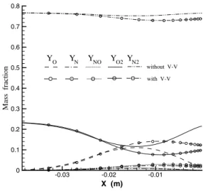
X (m)

M

as

s

fra

ct

io

n

-0.03 -0.02 -0.01 0

0.1 0.2 0.3 0.4 0.5 0.6 0.7 0.8

Y Y Y Y Y

with V-V without V-V

O N NO O2 N2

The rise of temperature observed near the wall involves a greater dissociation of the nitrogen and oxygen mole-cules in the case of V-V coupling. The vibrational tem-peratures take part in the calculations of forward reaction rates. Fig. 10 shows a discrepancy of dissociation of approx-imately 52.38% forO2and 3.52% forN2at the stagnation point. This high dissociation ofO2compared toN2can be explained by the fact that theO2molecules dissociate more quickly thanN2.

θ

Cf

0 10 20 30 40 50 60 70 80 90 0

0.02 0.04 0.06 0.08 0.1 0.12 0.14

Frozen Without V-V With V-V

Figure 11. Friction coefficient, Mach 20,Re= 4323.6.

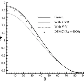
θ

Cp

10 20 30 40 50 60 70 80 90 0.2

0.4 0.6 0.8 1 1.2 1.4 1.6 1.8 2

Frozen

With CVD With V-V

DSMC (Re = 4000)

Figure 12. Comparison ofCp, Mach 20,Re= 4323.6.

The evolution of coefficientsCf,CpandChare given in

Figs. 11, 12 and 13 as a function of the angleθ. The chemi-cal reactions affect the thickness of the shock layer and one notes a decrease of the friction coefficient peak. The peak

difference between calculations with coupling CVD and V-V is about 4.5%. The comparison of the pressure coefficient predicted between DSMC and this calculation is shown in Fig. 12. One notes a good agreement (2.12% of difference). In Fig. 13, the maximum value of the heat flux is located to the position θ = 0o_{. The importance of the}

dissocia-tion reacdissocia-tions (endothermic) more accentuated in the case with V-V is remarkable on the wall heat flux. One observes a diminution ofCh of about 12.12% between the 2 cases.

The difference of about 15.38% is also observed between the DSMC and this calculation at the stagnation point for frozen solution. This divergence may be explained by the initial conditions of simulation, because the conditions of

Ma= 20andRe= 4000can be obtained at altitude having

different thermodynamic variables. Moreover, results pre-sented are withMa= 20andRe= 4323.6.

θ

10 20 30 40 50 60 70 80 90 0

0.1 0.2 0.3

Frozen

With CVD

With V-V

DSMC (Re = 4000)

Ch

Figure 13. Comparision of coefficientCh, Mach 20,Re= 4323.6.

Case Mach 25

When the Mach number increases for the same altitude, the enthalpy increases and the ionized particles become im-portant behind the shock wave. The air plasma surrounding re-entry vehicle may perturb the communications with the ground control, because plasma absorbs radio waves[19]. The objective of this section is to numerically study the in-fluence of the ionized particles and the electronic excita-tion on the aerothermodynamics parameters. For that, an equation of electron-electronic relaxation and two additional species are taken into account (N O+

ande−_{). The choice of}

N O+

is justified by the fact that the first energy of ionization (energy required to cause ionization) ofN Ois smallest. The flow are analysed thermally by using a model with four tem-peratures (T,TvO₂,TvN₂,Te). The chemical kinetic model

used for seven air species with 24 elementary reactions is proposed by Park[12].

The distribution of temperaturesT,TvN₂ andTeare

electronic excitation can be appreciated. One notes a de-cay of 12.25% of maximum of the translational temperature behind the shock wave cause by the translation - electronic coupling (T −E) which is defined here by Appleton and Bray[17]. The electronic - vibration coupling (E−V ), ac-cording to the Landau - Teller[5] model, concerns only the nitrogen molecule in this work, its influence on the evolu-tion of TvN₂ in the stagnation region is significant with a

fall of the temperature (≈ 23%). The skin friction coeffi-cient decreases with the nonequilibrium effects as shown in Fig. 15. The wall heat flux is represented on Fig. 16. One notes an increase in heat flux of about 4.41% inθ= 0o_due

to the electronic contribution. The taking into account of the thermochemical effects and their couplings brings a diminu-tion of 19.04% of heat flux at the stagnadiminu-tion point between frozen and nonequilibrium calculation.

X (m)

Temp

er

atu

res

,

[°K

]

-0.03 -0.02 -0.01 0

0 2000 4000 6000 8000 10000 12000 14000 16000 18000 20000

T TvN2

without electronic with electronic

Te T_vN2 T

Figure 14. Temperatures distribution along the stagnation line, Mach 25,Re= 5404.5.

θ

0 10 20 30 40 50 60 70 80 90

0 0.02 0.04 0.06 0.08 0.1 0.12 0.14 0.16 0.18

With electronic

Without electronic

Frozen

Cf

Figure 15. Friction coefficient, Mach 25,Re= 5404.5.

θ

0 10 20 30 40 50 60 70 80 90

0 100 200 300 400 500 600 700 800 900

Q(

K

W

/m

)

w

2

With electronic Without electronic Frozen

Figure 16. Wall heat flux, Mach 25,Re= 5404.5.

5

Conclusion

This work is based on a series of numerical and fundamental studies of the flow around reentry satellite SARA in order to better predict the true importance for the thermal protection. The physical model accounted thermochemical nonequilib-rium processes with a partially ionized gas. A robust 2D multiblock MUSCL-TVD finite volume scheme is used to solve the viscous flow at high Mach number. The correc-tion of the speed of sound due to the presence of the elec-tron temperature is also included. The various features of this complex flow are observed. The importance of the ther-mochemical phenomena on the aerothermodynamics para-meters is pointed out. In the frozen case, the results show a good agreement forCpandChwith the DSMC calculations.

The consideration of the thermochemical nonequilibrium ef-fects allows to be more close to the physical reality within the flow and improves the prediction of results.

In a future work, the radiative phenomena will be in-cluded in the model.

References

[1] F. Sharipov, Braz. J. Phys.33, 398 (2003).

[2] C. Park and F. K. Milos,Computational Equations for Radi-ating and AblRadi-ating Shock Layers. AIAA paper 85-0247, Jan-uary 1985.

[3] Lee Jong-Hun, Basic Governing Equations for the Flight Regimes of Aeroassisted Orbital Transfer Vehicles.Thermal Design of Aeroassisted Orbital Transfer Vehicles, H. F. Nel-son, ed., Volume 96 of progress in Astronautics and Aeronau-tics, American Inst. of Aeronautics and AstronauAeronau-tics, Inc., c.1985, pp. 3-53.

[5] W. G. Vincenti and C. H. Kruger Jr.,Introduction to physical Gas Dynamics.Krieger, FL, 1965.

[6] C. R. Wilke, Journal of Chemical Physics,18, 517 (1950). [7] J. D. Ramsaw, and C. H. Chang, Plasma Chem Plasma

process,13, 489 (1993).

[8] P. Roe, Jour. Comp. Phys.43, 357 (1983).

[9] Y. Burtschell, M. Cardoso and D.E Zeitoun, AIAA Journal,

39, 2357(2001).

[10] G. Tchuen, Mod´elisation et simulation num´erique des ´ecoulements `a haute enthalpie: influence du d´es´equilibre ´electronique. Th`ese de Doctorat de l’Universit´e de Provence - France, Novembre 2003.

[11] A. K. Hoffmann, T. S. Chiang, S. Siddiqui and M. Papadakis,

Fundamental Equations of Fluid Mechanics.A Publication of Engineering Education System, Wichita, Kansas USA, 1996.

[12] C. Park, Nonequilibrium Hypersonic Aerothermodynamics.

New York, Wiley 1990.

[13] G. Tchuen, Y. Burtschell and D.E Zeitoun,Numerical predic-tion of weakly ionized high enthalpy flow in thermal nonequi-lirium.AIAA Paper No. 2004-2462, 2004.

[14] G. V. Candler and R. W MacCormarck, Journal of Thermo-physics and Heat Transfer,5, 266 (1991).

[15] P. A. Gnoffo, A Code Calibration Program in Support of the Aeroassist Flight Experiment.AIAA Paper No. 89-1673, 1989.

[16] C. Park, Journal of Thermophysics and Heat Transfer,2, 8 (1988).

[17] J. P. Appleton and K. N. C. Bray, J. Fluid Mech. 20, 659 (1964).

[18] E. A. Masson and Monchick. The Journal of Chemical,36, 1622 (1962).