Piotr Rusek
PROFESSOR ANDRZEJ LASOTA’S THEORIES
IN ENGINEERING
Abstract. Professor Lasota’s achievements in the field of engineering are based on two prin-cipal aspects: profound theoretical backgrounds and perfect knowledge of phenomenological processes. That allowed him to solve many different problems of engineering.
1. FOREWORD
The deficiency of original theoretical solutions of engineering problems utilizing ad-vanced mathematical theories might be attributed to the certain pragmatism of en-gineers’ approach. Most professionals tend to think that theoretical works help but little to achieve practical results. Obviously, we do not have in mind the theories and analytical formulas that have been well proved in engineering practice, but the new theories from fast-changing fields of modern technology. Moreover, production engi-neering seems to defy research efforts. The lack of clear, practical theories is mostly due to the fact that many technological processes are accompanied by very complex, not well recognised physical and chemical phenomena. In order to obtain reliable re-sults in the theory of production engineering, profound theoretical backgrounds have to be supported by the perfect knowledge of phenomenological processes. Apparently, Prof. Lasota’s achievements in the field of engineering are based on these two aspects to guarantee full success. I was lucky to be able to be Prof. Lasota’s assistant during his engineering exploits.
2. TECHNOLOGY OF ROCK CUTTING
In 1968 the research program was undertaken in the Department of Manufacturing at AGH to study rock workability using cogged bits. This was a part of a vast research project commissioned by the drilling sector in Poland. No analytical method was available to determine the constraints of process parameters. First of all, it was necessary to determine the critical rotational speed of cogged bits which caused the
failures and consequent damage to the drilling tools, because in practice, parameters of the drilling process: the rotational speed and axial loading onto the cogged bits were determined from the fieldwork only.
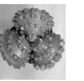
The primary tool used for deep holes drilling (hundreds to thousands of meters deep) is the cogged bit. A cogged bit incorporates toothed rings placed on conical surfaces rolling and pressing on the hole bottom (Fig. 1).
Fig. 1. Cogged bit: 1 – body; 2 – cogged roller; 3 – bearing
the centres located at the distance T = 2Rsinϕ. This curve, called the fundamental curve, is given by the formula:
z=p(x)
where p(x) =pR2−(x−a
k)2 for kT ≤x≤(k+ 1)T,
ak = (k+12)T, k= 0,1,2, . . . .
(1)
Fig. 2. Ejgieles’s model of a cogged bit
As regards ring performance, the following quantity is of key importance:
λ=ν 2M
F R ,
which is Froude’s number for this system.
It is worthwhile to mention that for λ <1 the ring centre moves precisely along the fundamental curve. In order to prove this, we need to show that the component of the reaction forceAz in the direction of thez-axis should be positive
Az=M
d2
dt2p+F.
It follows from equation (1) thatd2p/dx2=−R2/p3and hence:
d2
dt2p=ν 2 d2
dx2p=−
R2ν2
p3 .
Finally, for the componentAz we get:
Az=−
M R2ν2
p3 +F ≈ −
M ν2
Forλ >1, the componentAz in the direction ofz-axis is negative, which implies that in the period between two subsequent tooth-ground contact points the ring centre
C moves above the fundamental curve, in accordance with the formula:
Md
2z
dt2 =−F; therefore,
d2z
dx2 =−
F
M ν2. (2)
Trajectory of the pointC is derived as on Figure 3.
Fig. 3. Determining the sequence of node points {x}. Trajectory z = z(x) in the range (xi, xi+1) becomes the solution to equation (2) and at points xi it is a tangent to the
fundamental curvez=p(x)
Let us assume that at the initial point x=x0 (0≤x0< T) the solutionz(x)to equation (1) satisfies the following conditions:
z(x0) =p(x0), z′(x0) =p′(x0).
They imply that at the initial point the trajectory begins on the fundamental curve and will be tangent to it. This solution is valid to the right of the point x0as long as the conditionz(x)> p(x)is satisfied. The first intersection pointx1> x0 is found forz(x1) =p(x1). This procedure is then repeated, starting from the pointx1, which implies solution of equation (1) with the initial conditions:
z(x1) =p(x1), z′(x1) =p′(x1).
Let us then find the nearest point x2 > x1 where the solution intersects the fundamental curve. The next starting point is taken asx=x2, and pointx3is to be found in the same manner. Applying the recurrent procedure, we get the sequence of points:
Those points are called the node points of a trajectory. They correspond to sub-sequent impact points when the tool hits the bottom hole. Forλ <1 the trajectory results from kinematic excitations (z(x) = p(x)), so in this case node points will coincide with refraction points of the fundamental curve, it means:
xn=nT, n= 1,2, . . . .
Forλ= 1we get the first critical velocityvI:
v2I =HR, where H= F+M g
M
at which the reaction force componentAz becomes 0. ExceedingvI, the tool leaves the trajectory of fundamental curve, which vastly impacts on drilling performance. At lower velocities (λ <1) the tool operation is stable and the production rate increases with the rotating speed. At higher velocities the tool partly loses contact with the hole bottom and the trajectory of tool motion becomes most complicated (see Fig. 3). It is well proved [2] that in the range1< λ <2the tool motion remains stable even though the tool-ground contact is partly broken. Forλ= 2we get the second circumferential critical velocityvII.
vII2 = 2HR.
Above the velocity ofvII, the motion is no longer stable. It appears that the transition from stable to unstable motion is associated with the critical value of Froude’s number. At higher values of Froude’s number the system does not display any stable periodic trajectories. It is an analogon to turbulent flows of fluids at high Reynolds numbers. For small values of Froude’s number in stable motion, simple methods of analysis suffice to determine the operating parameters of the tool, particularly the mean energy transmitted to the ground by the tool. For higher values of Froude’s numbers (λ >2), the periodic trajectory is not stable (Fig. 4) and hence the methods of ergodic theory are recommended.
Fig. 4. Typical trajectory of a centre point of a single-ringed tool in unstable motion (λ >2)
To analyse this function, let us consider the existance of invariant measure for the dynamic system formerly described. Assuming that a physical quantity f might be expressed as a function of nodal points and can be written asf(bsn),its average value along the trajectory becomes:
f = lim n→∞
1
n
n X
k=1
f(sbk) = lim n→∞
1
n
n X
k=1
In accordance with Birkhoff-Chinczyn’s ergodic formula, the average value of f
along the trajectory is equal to the average value of f with respect to an ergodic invariant measure (for almost eachs0). Accordingly, we get:
f = Z 1
0
f(s)µλ(ds),
where µλ stands for an invariant measure. How to determine this measure was one of the major theoretical issues associated with the solution given by A, Lasota and J.Yorke [3] in relation to Ulam’s hypothesis concerning the existence of invariant measures for expanding transformations. In accordance with Ulam’s hypothesis, such measure exists [4] as long as the function τλ satisfies the condition |dτλ/ds| >1 at fixed points. That happens whenλ >2. As it was shown in [3], the condition:
inf s dτ2 λ(s)
ds
>1
is sufficient for ensuring the existence of an invariant measure. The given invariant measure being known, one might proceed to obtain [5] some of the process parameters, utilising the Birkhoff-Chinczyn’s individual ergodic theorem.
Remark 1. In order to find the measureµλ, the specific form of the individual ergodic
theorem is applicable:
lim n→∞ 1 n n X k=1
χD(τλ2(s)) =µλ(D),
whereχD denotes the characteristics function of the setD.
This formula might be used to analytically determineµλ(D). The calculations were
performed at the Institute of Fluid Dynamics of the Maryland University (USA). It turned out thatµλdistributions obtained numerically resemble the gamma distribution
with the density gbp(s). Thus obtained numerical data were further utilised to derive
the basic operating parameters of the cogged bit: the average impact energy and mined rock volume per one tool revolution.
In order to calculate an energy of the impact:
En = 1 2M dz dt 2 t=tn
at the momenttn which corresponds to the nodal point of a trajectory, we are going to use non-dimensional variables. The following results were obtained:
If 0< λ <1 then E=λK,
If 1< λ <2 then E=λ−1K,
If λ >2 then E=KR01(1−2s−2λ−1r
λ(s))2gbp(s)ds,
(3)
forK=1 2F Rsin
Another indicator of particular interest is expressed as the average volume of mined rock per one tool revolution, designated as h0. Let us assume after N.N Dawidenko [6] that the volume of rock mined during one tool impact is proportional to impact energyE, and can be written as:
h0=ρνE,
where: ν, ρ- the average number of impacts per revolution and the proportionality factor, respectively.
Next, the formula forh0 is obtained:
h0=
λK1 for 0< λ <1,
λ−1K
1 for 1< λ <2,
K1 R1
0(1−2s−2λ −1
rλ(s))2gbp(s)ds
R1 0λ−
1
rλ(s)gbp(s)ds for λ >2,
(4)
whereK1=14πdρFsinϕ.
The analysis of h0 for large λ, yields an asymptotic value which h0 approaches whenλtends to infinity. Namely, we get:
lim
λ→∞h0≈0,65K1.
It appears that the theoretically predicted relationship between mined rock volume per one tool revolution and the rotating speed agree very well with the well-known experimental data [7]. It is worthwhile to compare the experimental and theoretically predicted relationship between – h0 and n– the cogged bit’s rotating speed (Fig. 5 and Fig. 6).
Remark 2. For easy reference, there is velocitynof the rotational drilling in rpm on
the abscissa, instead ofλ. The relation between these two quantities is straightforward:
λ=M ν 2
F R = π2d2M
F R
n 60
2
,
wheredis the cogged bit diameter (hole).
Good correspondence between the theoretical results and industrial data allowed the reliable engineering computations, prompting further research leading to the de-sign of a new tool known as an isoangular bit.
The analysis of the cogged bit performance reveals that its elements tend to wear and tear quickly, as a result of impact. The tool itself is described by three functions:
N =f1(σ), σ=f2(E), υ=f3(E),
where:
N − number of cycles required to damage the tool (fatigue damage),
σ − maximal stress observed during one cycle in the worn part,
E − energy of a single impact,
Fig. 5. Experimental relation: mined rock volume –h0 per one tool revolution for the cogged bitΛ∆10-132
Fig. 6. Theoretical relationship between rock volumeh0 per one revolution and rotational speed n. The broken profile is derived from theoretical data; the continuous profile is the
Functionsf1,f2,f3are sufficient to determine the tool’s fatigue endurance and the total amount of mined materialV, given the predetermined constant energy. Thus:
N =f1(f2(E)) and V =N·υ=f1(f2(E))f3(E) (σis reduced).
The Palmgren hypothesis is applied to determine how effects of wear should cu-mulate under the variable energy of a single cycle:
k X
i=1
ni
Ni
= 1, N = k X
i=1
Ni,
where:
Ni − number of cycles (under stress σi required to damage the tool,
ni − number of cycles operated under the stressσi.
Whilst the tool is in service, positive effects (mined material) add to negative ones (loss of tool life measured by a number of cycles). After the boundary transition, the Palmgren hypothesis can be expressed with integrals:
N =
Z ∞
0
n(E)dE,
Z ∞
0
n(E)dE f1(f2(E))
= 1, V = Z ∞
0
f3(E)n(E)dE.
Bringing up a normalised distribution functionv(E) =N−1n(E), we get: Z ∞
0
v(E)dE= 1, v(E)≥0, (5)
1
N =
Z ∞
0
v(E)
f1(f2(E))
dE, (6)
V = R∞
0 f3(E)v(E)dE R∞
0
v(E)dE f1(f2(E))
. (7)
The numerator in expression (7) has a simple physical interpretation; this is the average productivityUb per one cycle
b
U = V
N =
Z ∞
0
f3(E)v(E)dE. (8)
Formulas (5), (6), (7) highlight the following optimisation problem.
Problem I
Problem II
Given the functionsf1, f2, f3 and the average cycle productivityU ,b find the distri-bution v to ensure the maximal total performanceV. (The solution to this problem suggested by Andrzej Lasota gave rise to many practical applications in the design and operation of impact tools, including cogged bits).
The solution proposed by Andrzej Lasota in his work [8] shall briefly be outlined. For simplicity, let us write1/f1(f2(E)) =f0(E). It is assumed that functionsf0 and
f1 belong to the class C2 forE ≥0. It is readily apparent that in considered func-tionals (5)–(8), the functionv is linear and hence those functionals are independent of its derivatives. That is why conventional methods of calculus of variations shall not apply and from the standpoint of Euler’s equations, it becomes a very specific case. Besides, even for very regular functionsf0, f1, the optimal distribution density
ν cannot be chosen from the set of functions but from the set of distributions, in accordance with the following theorem:
Theorem 1. Let f3(E) and f0(E0) be C2 class functions for E ≥0 and let υ and
E0 be stationary positive numbers such that the following condition is satisfied: Z ∞
0
f3(E)δ(E0−E) =f3(E0) =U . (9)
If
f′′
3(E)
f′
3(E)
<f
′′
0(E)
f′
0(E)
, f′
3(E)>0, f
′
0(E)>0 (10)
then the distribution ν(E) =δ(E0−E)shall implement the maximum of the integral Z ∞
0
f0(E)ν(E)dE
on the set of all distributions satisfying condition (5) and the condition:
Z ∞
0
f3(E)dE=U .
(The proof is provided in the Appendix to the paper [8]).
The theory of impact tool operation was applied to the design of an isoangular cogged bit, under Prof. Lasota’s instructions (Fig. 7).
Fig. 7. Tooth design in an isoangular bit to ensure uniform impact energy whilst in service
3. MACHINING OF METALS
Metal cutting processes are of key importance in mechanical engineering. High stan-dard surface qualities are often required. The achievements of modern engineering in a large degree depend on this surface quality. Vibrations occurring during the surface treatment negatively impact on surface quality. Numerous theoretical and practical studies highlight the evident relationships between vibrations and properties of the machined material, revealing the variable friction characteristics on the tool-machined surface contact, regenerative effects of vibrations occurring when the tool moves along the corrugated machined surface and dynamic properties of the machining tool. The most common source of vibrations accompanying nearly every machining process is the wear of the cutting tool (Fig. 8).
No earlier theoretical works are available that would highlight this particular cause of stability loss during the machining. Andrzej Lasota solved this problem basing on the theory of differential equations with a delayed parameter [9]. The simplest equation governing the tool vibrations is the following a linear equation:
md
2y
dt2 +b
dy
dt +cy=F(t), (11)
where:
m − reduced mass involved in vibrations,
y − cutting edge displacement normal to the axis of rotation of
a machined object and to velocity vector of the cutting process,
cy − elasticity force associated with machine tool rigidity,
F(t) − instantaneous thrust component of the cutting resistance force, actually, it is the instantaneous deviation of the thrust force
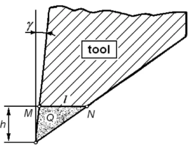
Fig. 8. Wear of a cutting tool OMN nearly triangular in shape
The force F depends on the profile of the machined surface near the cutting edge. Hence the natural transition to spatial coordinates (s, y) where s = vt. Assuming thatx(s) =y(s/v), wheres=vt(v-cutting speed) andF0(s) =F(s/v)equation (11) becomes:
mv2d
2x
ds2 +bv
dx
ds +cx=F0(s). (12)
The forceF depends chiefly on the profile of the machined surface along the section [s−l, s](Fig. 9).
For simplicity, let us assume that F0(s)is a linear functional and hence might be written as:
F0(s) =−k Z l
0
y(s−z)p(z)dz, (13)
where:
l − length of the section where the cutting edge contacts the machined surface,
k − coefficient expressing the cutting resistance,
Fig. 9. Distribution of the thrust component of the cutting force on the flank surface, where
l– length of the section where the cutting edge contacts the machined surface
Normalisation of the distributionpimplies that: Z l
0
p(z)dz= 1, p(z)≥0.
Equation (12) can be rewritten as:
mv2d
2y
ds2 +bv
dy
ds +cy+k
Z l
0
y(s−z)p(z)dz= 0. (14)
Substituting x= eζs to equation (14), where ζ =β+iω is a complex number, we get two characteristic equations, which are represented separately for the real and imaginary parts:
mv2(β2−ω2) +bvβ+c+kRl 0e
−βzcos(ωz)p(z)dz= 0, 2βωmv2+bvω−kRl
0e
−βzsin(ωz)p(z)dz= 0. (15) For small values ofl, the integrated function is expanded into Taylor series. Taking the linear terms only, we get a simplified system of equations:
mv2(β2−ω2) + (bv−kq)β+c+k= 0,
2βωmv2+bvω+kωq= 0, (16)
where:
q= Z l
0
zp(z)dz.
The parameterpis the mean value of distribution of the thrust force acting upon the cutting edge; it chiefly depends on the edge profile and can be written as follows:
q=εℓ, 1/3< ε <1/2
Solving equation (16) with respect tobyields:
β = 1/2m−1v−2(kεℓ
−bv).
The condition for the system to be stable is that β <0. In accordance with the presented theory, self-excited vibrations shall be generated when:
kℓε > bv. (17)
When the machine tool system becomes unstable, the surface quality of the ma-chined object will deteriorate. The common measure of surface quality after machin-ing treatment is the surface roughness. In normal, stable conditions, surface roughness
Ra is given by a fairly straightforward relationship:
Ra = 1
L
Z L
0 |
z(x)−< z >|dx, (18)
where: Ra – basic parameter of surface roughness, expressed as average deviation of a profile given by a functionz(x)from the mean-value line hzi, over the line section of length L.
For a widely applied profile shaped by a tool with the cutting edge in the form of a circular sector, we get:
Ra=
p2 18√3rε
(19)
where:
p − feed rate of the cutting tool,
rε − radius of the cutting edge producing the surface roughness.
Figure 10 shows typical experimental data revealing the roughness – advance rate relationship.
Major discrepancies between the experimental results, workshop practice and pre-dicted data are observed for small roughness which determine the quality of surface finish. These discrepancies might be attributable to vibrations. However, there were no theoretical works explaining how vibrations should impact on surface quality.
The model proposed by Prof. Lasota [10] for defining surface roughness in the conditions of vibrations occurrence was developed and proposed as it is shown in Figure 11 and finally written as equation (20).
zi(x) =ξi− 1 2rε
[(x−pi)−ηi]2, (20)
where: ξ and η – instantaneous displacements of the edge corner in the z and x
Fig. 10. Surface roughness Rz (Rz = 1.4−1.6Ra) vs feed rate when turning cylindrical bars made from carbon steel. Predicted relationships are indicated by broken line
Fig. 11. Roughness profile during the rolling in the conditions of transverse (x)and longi-tudinal(y)vibrations
Assuming thatξiandηifori= 1,2,3. . .are random variables,z(x)is treated as a stochastic process. QuantitieshziandRa might be computed when the distributions
ξiandηiare given. It is worthwhile to mention that only variances ofξiandηiare of key importance. The calculation procedure whereby all terms in order higher that the second as well as powers and products of moments of the order higher than the first are omitted as negligibly small in relation toσ2
For prevalent transverse vibrations:Ra=
p4 972r2
ε +50 81σ 2 ξ 1 2 .
For prevalent longitudinal vibrations:Ra =
p4 972r2
ǫ + 5p
2
162r2 ε
ση2 1
2
(very few occurrences).
To find the values ofσ2
ξ,ση2,it is required that vibration amplitude be determined, given the edge wearing and the stability conditions (17).
Thus obtained relationships reveal a good correspondence with workshop practice data and can be widely applied to design the surface finish operations and to determine the suitability of machine tools for use in operations to ensure the required surface finish standard.
4. ABRASIVE MACHINING
Andrzej Lasota’s interests in machining technologies prompted his research in abrasive cutting processes, particularly grinding - a basic process involved in finishing treat-ment. A chaotic distribution of cutting edges in the grinding process, a complicated mechanism of cutting involving cutting as well as friction and plastic deformations, rendered the theoretical research a formidable task. The first reliable theoretical re-sults were obtained thanks to the fundamental observation made by Prof. Lasota, who noticed an analogy between the Weierstrass function in the form given by B.R. Hunt [11] and the ground surface formation.
Remark 3. (Description of the Weierstrass function by B.R.Hunt)
z(x) =
∞
X
n=0
anh(bnx+θn),
where:
(θn) – is a sequence of independent random variables with a uniform
distribution over the interval [0, T] and T is an arbitrarily chosen positive number;
h(x) – is a periodic function (with the periodT) that should not be constant and must satisfy the Lipschitz condition.
Roughness profile generated after each passage of a cutting disc changes and so does the Weierstrass functionzn(x)becomingzn+1(x). Relating the constantsaand
of mathematics. Applications of fractals to the description of machining cases are now extensively studied by Prof. Lasota’s fellow researchers.
Finally, a few words about Prof. Andrzej Lasota from his student and later a fellow researcher. Mathematics that he dealt with would support engineering, was utilised to highlight major phenomena and processes and the rules of their occurrence. In his work he was a brilliant discoverer, not just a gifted performer. In his research work, he never took orders from anybody. He never worked for money, just by adjusting mathematical models to fit the existing laboratory data. He was always interested in problems that would show new horizons, both for theoretical research and workshop practice. His theories were always elegant and their beauty was evident even to us, engineers. He would never slight and diminish the role of workshop practice, which he always treated as a major reference point. Simplicity of final results allowed their easy implementation. His works are also most valuable in the teaching aspect, highlighting the links between theoretical results and commonly used engineering practice, hydro-dynamics, theoretical mechanics, strength of materials. His unfulfilled dream was a coherent theory of friction, he engaged in numerous experimental programs of great practical value though failing to provide a better insights into the physical aspects of friction. He was busy making plans, leaving notes and observations. Until the very end of his life he never ceased to be a most creative person, always encouraging and inspiring his fellow workers.
REFERENCES
[1] R.M. Ejgeles, K metodike raschiota riezhimow bureniya sharoshechnymi dolotami, Trudy MJJNH i GP im. J. Gubkina, Niedra 1967.
[2] A. Lasota, P. Rusek, Problemy stabilności pracy narzędzia w procesie wiercenia obro-towego świdrami gryzowymi, Archiwum Górnictwa 15, 1970.
[3] A. Lasota, J. Yorke, On the existence of invariant measures for piecewise mono-tonic transformation, Transactions of the American Mathematical Society186(1973), 481–488.
[4] S. Ulam,A collection of mathematical problems, Interscience Publish., Inc., 1960.
[5] A. Lasota, P. Rusek, Zastosowanie teorii ergodycznej do wyznaczania wydajności narzędzi gryzowych, Archiwum Górnictwa 19, 1974.
[6] L.E. Graf, D.J. Kogan, O.W. Smirnow, G.H. Fiedosiejew, Eksperimientalnoje issle-dowanije pieriedachi eniergii udara primienitielno k gidroudarnym mashinam kon-strukcji CKB Ministierstwa Gieologii SSSR, Rabota kolektiwnaya: Tieoriya i praktika udarno wrashchatielnogo burieniya, Niedra, 1967.
[7] J.E. Wladyslawliew, Issledowanije wlijaniya osiej sharoshok na pokazatieli raboty triexsharoshiechnyx dolot, Rabota kolektiwnaya: Tieoriya i tiekhnika burieniya, Niedra 1967.
[9] A. Lasota, P. Rusek,Stability of self-induced vibrations in metal cutting, Proceedings of the Fifth World Congress on the Theory of Machines and Mechanisms, Montreal, 1979.
[10] A. Lasota, P. Rusek, Influence of random vibrations on the roughness of turned sur-faces, Journal of Mechanical Working Technology, Elsevier Scientific Publishing Co.7 (1982/1983), 277–284.
[11] B.R. Hunt,The Hausdorff dimension of graphs of Weierstrass functions, Proc. Amer. Math. Soc.126(1998) 3, 791–800.
[12] W. Brostow, A. Lasota, P.Rusek, Description of surfaces for tribology, International Conference Baltrib 2007 Kaunas, Lithuania: Proceedings (Lithuan University of Agri-culture) (2007), 130–133.
Piotr Rusek [email protected]
AGH University of Science and Technology Faculty of Mechanical Engineering and Robotics al. Mickiewicza 30, 30-059 Kraków, Poland