A Game Theory Approach to Stock Lending Transactions in the
Brazilian Stock Market*
Kym Marcel Martins Ardison
Master student in Economics, Graduate School of Economics, Fundação Getulio Vargas E-mail: [email protected]
Luciana de Andrade Costa
Assistant Professor, Graduate Program in Economics, University of Vale do Rio dos Sinos E-mail: [email protected]
Received on 3.12.2013- Desk acceptance on 3.25.2013- 2nd. version approved on 5.15.2014
ABSTRACT
In Brazil’s market, the institution of interest on equity transactions provides a precedent for gains resulting from the difference between the tax rates of individuals (natural person) and those of investment funds through structured transactions. This difference creates incentives to lend stock; on the eve of an interest payment on equity, individual investors lend their stock to investment funds, which receive the interest in full and return only 85% of its value to the investors. Our goal is to understand how the surplus generated in this tax arbitration is split among the agents involved in the stock-lending transaction and to determine whether there are conditions under which the agents would have no incentive to conduct such a transaction. Using a non-cooperative games approach, we have structured this transaction and analyzed possible subgame perfect Nash equilibriums in three situations: (1) a direct relationship between the investor and the investment fund and an absence of transaction costs; (2) a direct relationship between the investor and the investment fund and the presence of tran-saction costs; (3) a relationship between the investor and the investment fund through a broker and the presence of (lower) trantran-saction costs. In the cases in which the broker does not mediate the relationship, more contracts tend to be signed, but the fund’s gain will only cover the record-keeping costs of the transaction. This situation is reversed in the presence of high transaction costs: in extreme cases, the investor loses bargaining power and his/her gain compensates only for his/her risk aversion. When a broker is introduced into stock lending, only those investors who have a minimum amount of stock will receive offers from the fund through the broker. The fund’s gain tends to decrease due to the broker’s presence and in some situations, the investor loses bargaining power and accepts any contract that compensates for his/her risk aversion.
Keywords: Interest on equity. Stock lending. Bargaining games.
1 INTRODUCTION
This study develops a theoretical model of the sto-ck lending of companies registered with the São Paulo Stock Exchange (Bolsa de Valores, Mercadorias e Futu-ros—BM&F Bovespa) that take place between indivi-dual (natural person) investors and investment funds in periods preceding payments of interest on equity. Like dividends, interest on equity is a means for a com-pany to distribute proceeds. However, the differences between different types of proceeds include the fact that, unlike dividends, companies are exempt from paying taxes on distributed interest on equity and that, moreover, the individual stockholder pays income tax on the proceeds that he or she receives in the form of interest on equity.
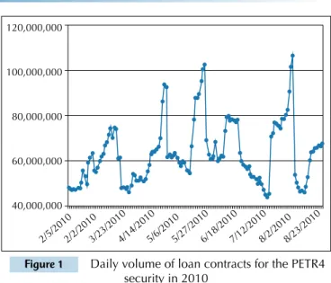
The primary motivation for this study arises out of the atypical movement in the volume of stock lending contracts on the Brazilian market on dates preceding the payment of interest on equity1. Despite the limited
availability of data about this market, we can verify this atypical movement in Figure 12-3 , where we present the
evolution of stock lending volume for Petrobras pre-ferred stock (PETR4). This movement is primary due to loan contracts between individuals and investment funds related to the tax gains derived from the inte-rest-payment transaction. Put simply, when interest on equity is to be paid, income tax falls on the security’s holder rather than on the issuing company, as in the case of dividends. In the case of individuals, the inco-me tax rate set by law is 15% of the interest on equi-ty value, whereas investment funds are exempt from paying the tax.
This taxation difference creates an opportunity for additional gain that can be exploited by individual in-vestors. We might structure a stock lending as follows: the individual investor lends his or her securities to an investment fund at a agreed annual rate for a pre-determined period of time preceding the payment of interest on equity. The investment fund then has the asset in its custody, receiving all proceeds related to it. Accordingly, when the interest on equity is paid, the investment fund receives its full value-i.e., without de-duction of income taxes, given that the fund is exempt. Moreover, when interest on equity is received, the in-vestment fund pays the individual investor the amount that he or she would have received if the stock had been in his or her custody-i.e., 85% of the interest on equity value. On the day after the asset pays the ex-interest on equity, the fund returns the stock to the individual in-vestor and compensates him/her through a previously agreed-upon loan fee.
Figure 1 Daily volume of loan contracts for the PETR4
security in 2010
Source: http://www.clubedopairico.com.br/aluguel-de-acoes-a-distorcao-jcp/5616
1 The ex-interest on equity date is set by the company: it is the date that the company will use as a base for paying interest on equity. In other words, all those who possess the relevant asset in their custody on the given
day will receive the interest. The actual interest on equity payment will not necessarily occur on that date.
2 Interest on equity EX payment dates: January 22, 2010, May 21, 2010 and July 30, 2010.
3 BM&F Bovespa provides daily data on loan contracts for each asset, but the time series for these data are not available.
By using the strategy just described, the tax gain related to the 15% income tax that would have been paid by the individual is no longer withheld. In this study, we are interested in ascertaining how this gain on the taxes is split. At first, we might think that the investor would extract the whole gain, minus the costs inherent to stock lending. This conclusion is primarily based on the idea that the investor that holds the sto-ck has bargaining power. However, when we introdu-ce the opportunity cost of offering loan contracts, we see that the investor, given a high cost that exceeds the transaction’s tax gain, will accept any contract offered by the fund that pays for his or her risk aversion. Mo-reover, when we consider the presence of a broker in-termediating the contract between the investor and the investment fund, we see that, as a result, the investor’s high-cost problem is reduced.
In this study, we seek to contribute to the literatu-re on inteliteratu-rest on equity by demonstrating, using the framework of bargaining games initially proposed by Rubinstein (1982), how individual investors can obtain additional profit by exploiting opportunities connec-ted to receiving interest on equity. The literature on interest on equity has investigated, from a company perspective, the incentives and determining factors re-lated to the choice of type of stockholder remuneration (Boulton, Braga-Alves, & Shastri, 2012; Minozzo, 2011; Brito, Lima, & Silva, 2009; Ness Jr. & Zani, 2001). In turn, Colombo and Terra (2012) study the characteris-tics of companies’ property structures that influence the interest on equity distribution from a beneficiary perspective. Likewise, the present study analyzes the
is-120,000,000
100,000,000
80,000,000
60,000,000
40,000,000
sue of interest on equity distribution from a beneficiary perspective. However, our approach intends to explo-re opportunities for individual stockholders to explo-realize additional gain when interest on equity is paid.
Our article is organized as follows. In the next sec-tion, we present the legal framework for stock lending.
In the third section, we provide a short literature re-view regarding aspects related to interest on equity and stock lending. In the fourth section, we present the proposed model and in the fifth section, we discuss the main results. Finally, we present our conclusions in the sixth section.
2 LEGAL CHARACTERIZATION
Stock lending4 essentially consists of lending the
secu-rities of publicly traded companies duly registered with the stock exchange. The natural or legal person who owns and is willing to lend a publicly traded company’s stock is called a lender. A lender will lend his or her stock to a borrower, who is also a natural or legal person, and who will have the stock in his or her custody once the lending transactions are consolidated. Moreover, BM&F Bovespa and a custo-dian institution - generally a brokerage firm - also partici-pate in the lending transactions. It is for BM&F Bovespa to register stock lending through the Security Lending Bank (Banco de Aluguel de Títulos - BTC) and to act as a coun-terpart in the transaction, ensuring the return of the asset and the due remuneration of the lender. The broker acts as intermediary in the lending transactions, connecting len-ders and borrowers and registering the transactions with the BM&F Bovespa system.
In stock lending, the lender (who has custody of the stock) abdicates his/her legal right over the asset and makes it available on the market. The borrower then gains rights over the asset and remunerates the lender for those rights at an agreed-upon rate, calculated as follows:
i
100
α = ( Q C* ) 1+ -1*
du
252
where α is the lender’s remuneration; Q is the stock amount being lent; C is the rate used in the loan; i is the remuneration rate defined by the lender; and du is the number of business days that the loan is in place. The re-muneration is always paid at the end of the loan period, which is defined before the contract is signed. In some fo-reseeable cases, contracts may be prematurely terminated by the lender, which should inform the borrower parties and provide them with a deadline of D+4 to return the assets in custody.
BM&F Bovespa charges a transaction registration fee of 0.25% p.a. on the transaction volume, in the case of loans willingly contracted by the borrower, with a minimum fee
of R$10.00. Moreover, the brokerage fee is agreed upon by the lender/borrower and the brokerage firm. It must also be pointed out that lending stock is defined as a fixed-income transaction for the lender and therefore is subject to the taxation stipulated in Law Number 11.033 (2004).
Some common characteristics shared by loan con-tracts deserve special attention. All custody events in cash, dividends and interest on equity are paid back to the lender by BM&F Bovespa as reimbursement, already fit to the corresponding taxation model, paid on the same day and in the same amount as the stock-issuing company’s payment. It must be stressed that according to Norma-tive Instruction Number 1,022 (Receita Federal do Brasil
- RFB, 2010), interest on equity and dividend values reim-bursed to the lender is considered to be a partial restitu-tion of the values lent, not gain, and therefore is tax free. The borrowing party should retain the amount paid to the lender available, as a guarantee, in its exchange balance. We further stress that although events related to stock custody (bonuses, etc.) are guaranteed to the lender in addition to stock subscription rights, we will not go into further detail because such events are beyond the scope of this study. Moreover, as an incentive, BM&F Bovespa guarantees the lender an additional gross profit of 0.05% p.a. on the lending volume.
Interest on equity is one of several means for stockhol-ders to receive remuneration. The interest on equity insti-tution is supported by article 9 of Law 9,249 (1995), which permits deduction of an interest on equity payment from a legal person’s income tax base. According to that law, taxes related to interest on equity are withheld at a rate of 15% for individuals. In addition, according to the Bra-zilian Federal Revenue Office (Receita Federal do Brasil; RFB, 2010), investment funds are exempt from paying taxes on interest on equity. Thus, we have the legal fra-mework necessary for the transaction to occur because by law, investment funds are free from taxes on interest on equity.
3 LITERATURE REVIEW
Company policy for stockholder remuneration is one of the most studied fields in corporate finance. In the literature, there is a consensus that Lintner (1956) and Gordon (1959) began the discussion. Those authors note that stock prices are directly connected to the flow of paid dividends. According to them, investors require lower
re-turn rates when dividends are high; in addition, they pre-fer the dividend upfront to decrease uncertainty.
Miller and Modigliani (1961) argue that in a scenario of no taxes, bankruptcy costs or asymmetric information and in which markets are efficient, dividend policy does not affect company value. In such a case, an investor would
4 Stock lending is regulated by Instruction Number 249 (CVM, 1996), which was later modiied by Instructions Numbers 277 (CVM, 1998) and 441 (CVM, 2006), the latter of which was further modiied by Instruction
be indifferent to the company's remuneration policy and company value would be affected only by its capacity to ge-nerate value and the risk inherent to its business activity.
Miller and Modigliani’s (1961) model is particularly interesting in Brazil because the law allows the remunera-tion of capital not only from tradiremunera-tional dividends but also from interest on equity. Interest on equity is seen, in part of the literature, as a variant of Allowance for Corporate Equity (ACE). According to Klemm (2007), the tax be-nefit generated by the interest on equity deduction when results are calculated is similar to the deduction allowed by ACE. However, the difference between the two resides in the fact that, in Brazil, the deduction is only permitted if interest is distributed to stockholders. Thus, we have a peculiar situation in which companies have the possibility of distributing proceeds in two distinct ways: dividends or interest on equity.
Furthermore, Libonati, Lagioia and Maciel (2008) have shown that because interest on equity payments lead to a reduction in tax burden, it is a better option for stockhol-der remuneration. Thus, viewing interest on equity as sto-ckholder remuneration contradicts Miller and Modigliani’s (1961) argument that remuneration policy is irrelevant. In such a case, one can easily observe that the investor would prefer to be paid via interest on equity because as stated by Libonati et al. (2008), interest on equity generates a tax reduction for the paying company and consequently, an in-creased propensity to directly remunerate the stockholder.
Increased incentive to direct remuneration as a func-tion of tax advantages also receives special attenfunc-tion in studies by Brito, Lima and Silva (2009), Futema, Basso and Kayo (2009) and Dos Santos (2007). Brito et al. (2009) note that as of 1996, there has been a 50% increase in the number of companies distributing their profits (whether as dividends or interest on equity) to stockholders. Cor-roborating this evidence, Dos Santos (2007) shows that since 1996, there has been a substantial increase in the percentage of (primarily publicly traded) companies that have opted for remuneration via interest on equity. The author finds that approximately 42% of companies sur-veyed have resorted to paying interest on equity as a me-thod of remunerating stockholders.
Looking at the option for paying proceeds via interest on equity from another perspective, Ness Jr. and Zani (2001) demonstrate not only that there is a tax advantage when using interest on equity but also that this adds va-lue to companies. However, contrary to expectations, the authors conclude that the benefit does not translate into a change in companies’ preferences related to the type of
capital chosen for financing.
Boulton, Braga-Alves and Shastri (2012) also find evi-dence in the Brazilian market that taxes are the primary determinant of stockholder remuneration policy. Those authors show that increases in profitability and payout ra-tio raise the likelihood of a company directly remunerating stockholders using interest on equity instead of dividends.
As can be observed from the cited works, a substantial proportion of the Brazilian literature discusses interest on equity payments from a company perspective. Similar to Colombo and Terra (2012), the goal of our study is to ex-plore an additional benefit related to interest on equity payments from a stockholder perspective. In their work, Colombo and Terra (2012) investigate the relationship between the property structure of companies listed on the stock exchange and interest on equity distribution. Taking into account the different tax incentives generated by the interest on equity payment (given different tax rates for different investors), the authors find evidence that both a company’s capital structure and its controller influence the interest on equity distribution.
Colombo and Terra (2012) also discuss the advantages re-lated to taxing the interest on equity beneficiary. The authors point out that in the case of investment funds, there is an addi-tional advantage of an interest on equity payment: their tax rate is zero. The exact goal of our study is to model a lending transaction that originates from this difference in the way that taxes are imposed depending on the type of investor, thus con-tributing to closing the gap in the literature regarding this type of study, as pointed out by Martins and Famá (2012).
This opportunity for tax arbitration is pointed out by Fraga (2013), who finds a positive effect of interest on equity payments on stock loan balances. That author further notes that stock-lending transactions conducted to exploit this difference in tax rules can affect share pri-ce formation, given that tax gains may be unevenly split between lender and borrower according to the investor’s bargaining power. Our model seeks to define the mini-mum number of shares that would prompt an investor to lend them, along with the situations in which he or she would lose part of his or her bargaining power. By doing so, we intend to explain part of the movement that has been observed in Brazil’s security lending market, which according to Minozzo (2011) has gained importance and liquidity. The importance of this market’s development was pointed out in the pioneering work by Diamond and Verecchia (1987) as a way to increase market efficiency, given that restrictions on short sales would imply slower adjustments to stock prices because of new information.
4 THEORETICAL MODEL
The game theory literature is divided into cooperative games, in which game participants’ strategies are coordi-nated so that the best outcome for the group as a whole may be achieved, and non-cooperative games, in which each individual makes decisions to maximize his or her own payoff. Our study uses the conceptual approach of
each player i as a function of their strategies; and a set of actions at each node in which the player is called to play.5
Based on these definitions, we now define the game that we are interested in analyzing. It consists of three players {fundo de investimento (FI),investidor
(I),corretora (C)}. Their respective sets of actions are
AFI= {offers a contract, does not offer a contract, ac-cepts counterproposal, rejects counterproposal},AC
={forwards the contract offered by the fund, does not forward the contract offered by the fund, forwards the investor's counterproposal, does not forward the investor's counterproposal} and AI ={accepts contract, rejects contract and makes counterproposal, rejects contract and does not make counterproposal}.
In general, we have six decision nodes in this game. The investment fund plays in the initial node, choosing whether to offer a contract. The broker plays in the se-cond node, deciding whether to forward the contract to the investor. In the third and fourth nodes, the investor plays. First, the investor decides whether to accept the contract. In case of rejection, he or she decides whether to make a counterproposal. The broker plays again in the fifth node, deciding whether to forward the counterpro-posal to the fund. Finally, in the sixth node, the fund plays and decides whether to accept the counterproposal. The payoff function will be defined later for each player.
Based on this sequence of moves, we consider that in a game Γe , a strategy σ
i is termed “of best response” for player i in the face of rival players’ strategies σ-i if u(σi,
σ-i)≥u(σ'i, σ-i), for every σ-i in other players’ sets of stra-tegies. Therefore, we solve the game by means of a ba-ckward induction process defined as follows: starting from a terminal node T, we identify the best action for the player playing at T-1. Next, we defined a reduced game Γe in which at T-1 , we substitute the payoff, referring to
the previously defined strategy. We carry out this inducti-ve process until we reach the initial node. Giinducti-ven that our game is finite and contains perfect information, the ba-ckward induction process will take us to one of the game’s possible subgame perfect Nash equilibriums (SPNE).
Once we have described the game’s primary elements and the method used to describe possible equilibriums, our goal is to determine how this lending transaction’s ag-gregate gain, which is a function of the difference in taxa-tion between investment funds and individual investors, is split between the parties involved in it. Thus, we are initially interested in identifying the necessary conditions for the stock lending contract to be effected, given the existing cost constraints, and then to determine how the transaction’s aggregate profit (deducting brokerage costs) should be split among the players.
When the lending transaction takes place, the investor’s gain is expressed by the agreed-upon interest rate. In other words, in this game, the investor is remunerated through the interest rate paid by the investment fund. As
previou-sly described, interest received from stock lending is ta-xed as fita-xed income (we consider a rate of 22.5% because the lending duration is less than six months). Therefore, the investor’s net gain is the amount received for the loan (which depends on the agreed-upon interest rate) minus income taxes.
Conversely, the broker charges a fixed percentage of the stock lending volume. Therefore, given that a contract is signed, the broker is remunerated based on the broke-rage fee charged for the stock lending.
Finally, the investment fund’s claim is the transaction residual, in the sense that its net remuneration is the gross balance of the transaction minus the costs and remunera-tions paid to the broker and the investor.
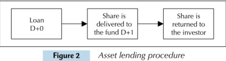
We initially model the game without the broker and then include the broker to compare the results. We assu-me that the investor is risk-averse. Therefore, the lending process starts one day before the stock becomes ex-inte-rest on equity and the security is returned on the day im-mediately after the stock becomes ex-interest on equity, as in Figure 2 below.
5 Adapted from Fudenberg and Tirole (1991).
6 Given the procedure above, the investment fund will have the security in its custody on D+1 and will return it to the lender on D+2.
Figure 2 Asset lending procedure
Assuming the procedure takes place in this manner, the lender’s risk is reduced because the asset is unavailable to the lender for negotiation for the shortest period possi-ble, but the minimum loan duration set by the BTC Bank6
is still respected.
We define the lender’s utility function as follows:
where α is the investor’s remuneration defined as a func-tion of the amount of stock (Q) in custody and the inte-rest rate (i) charged at the moment of lending. Parameter β captures the lender's risk aversion, σ2 is the historical volatility of the asset in question, and “"f ” is a function whose characteristics we will define shortly.
With respect to parameter β, we intuitively know that short- and medium-term investors only have su-fficient incentive to lend their assets if they believe that the implied remuneration will exceed the risk involved, given that the asset cannot be sold while it is lent. For long-term investors, this function’s parameter β will be relatively low, because such investors are less averse to short-term variations. This utility function is similar to that proposed by Levy and Markowitz (1979). In particular, we define utility as a linear function of the agent’s payoff (received via remuneration of the loan fee) and an exponential function of the volatility of the asset return. The investor’s remuneration function is
U(σ2, α) = α(Q, i) - βf(σ2) Loan
D+0
Share is delivered to the fund D+1
then defined by:
Notice that this function depends on the transac-tion volume given by Q P-1, where Q is the amount of stock lent and P-1 is the asset’s closing price on the eve of the loan contract. Considering how we have desig-ned the lending transactions, we have du=1, and thus we can define Ii as:
Substituting Ii in function α(Q, ii) we have:
Let the following be characteristics of the lender’s utility function: , , and . Such premises indicate that the lender’s utility grows, with decreasing marginal returns, as the lender’s remu-neration grows, and it decreases exponentially as the asset’s volatility (σ2) increases. We further define that f(0) =0.
The investment fund’s profit is defined as follows:
Notice that as we have previously described, the transaction’s tax gain essentially consists of the invest-ment fund’s tax exemption when it receives interest on equity payments. Therefore, given the income tax rate of 15% for individuals, we have a potential gain of 0.15*interest on equity. This means that the fund’s profit is a linear function of the interest on equity value, of α (share of tax gains that is passed onto the lending inves-tor) and of the cost associated with the registration fee charged by BM&FBovespa.
Our model assumes n individual investors and k in-vestment funds in the market and that all funds and inves-tor have full knowledge of the lending transactions. This premise may seem relatively restrictive at first, but we will show that it does not alter our results.
We consider that the investment fund offers a contract to the investor. Under the usual definition, both the len-ding investor and the investment fund will only accept the proposal if its 0 is such that U(σ2; α) > 0 and θ > 0.
Next, we present the three models that comprise our study. We analyze the behaviors of the investor, of the in-vestment fund and the broker, noting the implications of having an intermediary - in this case, the broker.
In all of the models presented next, we consider that the investment fund is the first to play. After observing the strategy chosen by the fund, the investor is called to play and to make his/her decision. It is important to stress that the results of the model are not altered by choosing the fund as the initial player. This choice was made only to standardize our reasoning and because ne-gotiations occur in this manner in the financial market.
ii
100
α(Q, ii) = ( Q P* -1) 1+ -1*
du
252
ii
100
Ii = 1+ -1
1
252
α(Q, Ii) = (Q P* -1) *Ii
∂U
∂α >0
∂U
∂f <0
∂2U ∂f 2 <0
∂f
∂σ2 >0
θ = 0.15 *JSCP *Q - α - MAX {10; 0.0025 * *Q C}
4.1 Model 1.
We initially assume no brokerage or intermediation costs, i.e., the funds and potential lending investors are free to negotiate with one another. This is a restrictive hypothesis because in the capital market, individual in-vestors (with relatively small capital) do not have direct contact with investment fund managers, and the broker plays an essential role intermediating that relationship. Later, we add the broker to the game and assess the effect of the broker’s presence on the results.
The game is characterized as follows: initially, the in-vestment fund offers a contract to the investor, which con-sists of a payoff for the investor and another for itself. Upon receiving the proposal, the investor chooses whether to accept or reject the contract. In the rejection scenario, the investor may or may not offer a counterproposal, or it may even offer a new contract to another fund. Observing the contract offered by the investor, the fund chooses whether or not to accept it.
Notice that this game may be played recursively, i.e., the fund may reject the investor’s proposal and offer another contract instead. For simplicity, we assume that if the fund rejects the investor’s proposal, the game ends, which is easy to verify because the investor offers the contract that is best for him/her. Assuming the fund will accept any contract with a positive payoff, the investor will not accept any other contract offered by the fund, and no other fund will accept the contract offered.
First, we must verify the transaction’s feasibility cons-traint. For the lending transaction to occur, the gain it generates must be greater than the registration costs. Therefore, as previously defined, we have the transaction’s maximum profit given by 0.15 IOE Q, where IOE is the interest on equity. The BM&FBovespa BTC defines that registration costs as the largest of R$10.00 or 0.25% of the contract’s total volume (Q P-1). The feasibility constraint is thus represented by:
From this constraint, we obtain two particular cases that should be analyzed. The first is that in which the registration cost does not exceed the minimum set by BM&FBovespa. In the second, the registration cost will depend on the contract’s volume.
4.1.1 Case 1.
In the first case, the transaction’s registration cost does not exceed the minimum required by BM&FBovespa, i.e.:
The feasibility constraint may then be written as:
so
0.15 *JSCP *Q - MAX {10; 0.0025 * *Q P-1}>0 1
0.0025 *Q P* -1< 10
0.15 *JSCP Q * > 10
*
Q > 10 2
0.15 JSCP
*
*
* *
This condition is intuitive because the larger the interest on equity paid by the company, the smaller the amount of stock needed for the lending transactions to become profitable.
4.1.2 Case 2.
In this case, the registration cost exceeds the minimum fee required by BM&FBovespa, so that the feasibility restric-tion is given by:
from which
This means that the lending transaction is profitable only if condition (3) is met. Notice also that in this case, the fea-sibility constraint does not depend on the amount of stock owned by the investor, but rather on the share price used when calculating the loan fee. Alternatively, pursuant to our definition of P-1 (as the asset's closing price in D-1), we have , which gives us a relationship that is similar to that of dividend-yield. Thus, the lending tran-saction is profitable only if the interest-yield ratio is greater than approximately 1.67%. Because of this, investors who negotiate large stock amounts are willing to lend them, de-pending on the return offered via interest on equity. Given the constraints derived in the two cases above, we may return to the game itself. We know that if the investor rejects the fund’s initial offer, the investor will offer a con-tract from which to excon-tract the most profit. Notice, howe-ver, that the investor only makes a new proposal if
We then require
where ψ is the value paid to the fund. Thus, the investor will only offer a contract when the benefit of doing so exce-eds his/her risk aversion. Assuming a Q that is sufficiently large, as in (3) ( ), isolating Q gives us:
We further note that the hypothesis of the knowledge of the lending transactions, which is apparently strong from the individual investor’s perspective, in reality is not very restrictive. Given that the game is a dynamic one, we can assume that once a fund presents its initial proposal to the investor, the latter learns about the lending transactions and has the freedom to offer new contracts to other funds.
Notice also that the investor chooses ψ (value offered to the fund in the contract) to maximize his or her gain, pro-vided the fund still accepts the proposal. Therefore, given the continuity of the fund’s profit function, we have that at the limit, the contract offered by the investor is such that:
Substituting (6) into (5):
0.15 *JSCP Q * > 0.0025 * *Q P-1
* 0.0025 P-1
0.15
JSCP > 3
U(σ2, α) > 0 4
*
(0.15 JSCP Q - ψ) 0.775 > βf (σ2)
* *
Q1 > βf (σ 5
2) + 0.775 ψ
0.775(0.15JSCP)
ψ = 0.0025 *Q P* -1 6
Q1 > βf (σ 2)
0.775(0.15 JSCP - 0.0025 P-1)
Thus, given the necessary conditions for the investor to offer the contract, he/she will do it and the fund will accept it, with payoffs ψ = MAX {10; 0.0025 Q P-1 } for the fund and (0.15 JSCP Q - MAX {10; 0.0025 Q P-1}) 0.775 for the investor. As we have observed, the fund accepts this contract, which consists of the Nash equilibrium for the subgame in which the investor decides to offer a new con-tract to the fund.
Finally, through backward induction, we know that the investment fund will offer exactly the same contract that the investor would choose if he were to reject the contract offered by the fund. By offering such a contract, the fund makes the investor indifferent as to whether to accept it and therefore, using Nash’s argument (1950) that time is “valuable”, the investor accepts the contract7.
4.2 Model 2.
Like Rubinstein (1982), we now consider that the agents (except for the investment fund) have a fixed cost for presen-ting a counterproposal. The fixed cost represents both the effective cost of drafting the contract and the agents’ opportu-nity cost of investing time to conduct the lending transaction. Thus, we add a cost CO to model 1 for the investor to offer a new contract. This is a reasonable hypothesis becau-se if the offered contract is rejected, the investor must find a new fund to which he can offer his contract.
Although it has been previously mentioned, following is another caveat: in Brazil’s market, brokers have an im-portant function as a link between investment funds and investors. In general, the largest fund managers do not have direct contact with potential investors. Moreover, investors have high costs associated with contacting such funds. Theoretically, however, under the hypothesis of there being no brokers, investors might be able to contact fund mana-gers directly.
In the presence of the cost of the offer, CO, should the investor reject the initial contract, we then face two chan-ges. The first has to do with the fact that the investor, should he/she offer a new contract to a fund, will have a maximum payoff such that:
This utility function defines which contract the fund should offer to render the consumer indifferent between the choices of either accepting the contract or rejecting it and seeking new options in the market.
We also know that the investor only offers a new con-tract if he/she obtains some positive utility from doing so. Therefore, we have a change in the investor’s participation constraint:
The game’s development in the case in which the profit resulting from the lending transactions is sufficiently high to cover both the investor's risk aversion and his/her costs for offering a new contract is similar to that of the previous case. We now look at the situation in which the lending transaction’s profit is sufficient to compensate the investor’s
7 We could also use a time-varying discount rate, but given that the negotiation usually occurs on the day that the interest on equity is paid, such a methodology would not be relevant. *
U(σ2, α)
max = (0.15 JSCP Q - ψ) 0.775 - βf (σ 2) - CO
* *
(0.15 JSCP Q - ψ) 0.775 > βf (σ2) + CO 7 *
* *
*
JSCP 0.0025 C 0.15>
10 0.15 JSCP Q >
*
* * * * *
risk aversion but insufficient to also cover the costs of offe-ring a new contract. Such conditions might be expressed as:
In this case, the maximum profit generated by the len-ding transactions does not cover the risk aversion cost added to the investor’s costs for offering a new contract. However, the tax gain is sufficiently high to cover the investor’s risk aversion.
We then have a situation in which the investor decides not to offer a new contract when he or she does not accept the one drafted by the fund. In this specific case, the investor does not have the power to bargain with the fund. Therefo-re, any contract offered by the fund that results in a positive utility for the investor will be accepted. For us to understand which factors affect such a contract, we can isolate Q in (8):
We also know that if the investor could offer a contract (should this represent a gain for him/her), he or she would do so, offering ψ = MAX{10;0.0025 Q P-1} to the fund. The-refore, substituting this into (10):
Thus, for amounts that are lower than this, the investor accepts any contract offered by the fund that remunerates his/her risk aversion, while the fund keeps all of the remai-ning tax gains of the lending transactions.
On the other hand, if the investor owns a sufficiently large stock amount, should he reject the fund's contract and offer another one, then his/her maximum payoff is given by:
Likewise, the offer made to the fund would be ψ=MAX{10;0.0025 Q P-1}
Replacing this in (11) gives us:
Finally, notice that if the fund offers a contract so that its payoff and
the investor accepts the offer because α=αmax.
In this case, the SPNE is such that the fund offers the contract described above and the investor accepts it, res-pecting the already described feasibility conditions.
4.3 Model 3.
In this section, we add the broker to the game. The broker plays the role of intermediary between the in-vestment funds and their clients. The presence of
(0.15 JSCP Q - ψ) 0.775 < βf (σ2) + CO 8 *
* *
(0.15 JSCP Q - ψ) 0.775 > βf (σ2) 9 *
* *
*
Q2 < βf (σ 10
2) + CO + 0.775 ψ 0.15 0.775 *JSCP
* * *
* * Q2 <βf (σ
2) + CO + 0.775 MAX {10; 0.0025 Q P
-1}
0.15 0.775 JSCP
αmax = (0.15 *JSCP Q - ψ* ) 0.775 - * CO 11
αmax=(0.15 *JSCP Q -MAX* {10; 0.0025 * *Q P-1}) 0.775* -CO 12
ψ = MAX{10; 0.0025 *Q P* -1} +Min0.775(CO,0)
* *
* *
*
α=(0.15 JSCP Q-MAX{10; 0.0025 Q P-1}- 0.775 Min0.775(CO,0)
brokers increases market efficiency because now, the contact between investment funds and investors is bridged by the presence of the intermediary institution, which effectively has information about the investors’ custody and even their risk profiles.
We assume that the broker must decide whether or not to contact its clients to offer the fund’s contract. Conside-ring that the brokerage market operates in monopolistic competition8, the broker's profit function is given by:
where γ(Q) is the broker’s revenue as a function of its client’s stock amount and CT is the broker’s cost for con-tacting the client and offering the fund’s contract. It is im-portant to stress that the broker is paid only if the loan contract is executed.
In Brazil’s market, stock lending transactions are cha-racterized by the absence of brokerage. Brokers are essen-tially paid out of the spread between the fee charged from the borrower and the fee paid to the lender. Therefore, we can define γ(Q) as follows:
We start from the premise that ic is externally defined. This hypothesis is reasonable because in general, brokers have a spread to charge in the lending transactions at the time it is structured. We can further interpret ic as a brokerage percentage that varies in accordance with the amount of stock owned by the investor.
As previously defined, we know that du=1, and there-fore, we can simplify the broker’s revenue function as:
where Ic, is the fee charged by the broker as spread in the period (in this case, one day). Given the hypothesis that the broker sets a spread fee to be charged in the lending tran-sactions, it offers the contract to its client if and only if:
We thus have that:
This means that the broker will only have sufficient incen-tive to offer the contract to the investor if the amount of stock that the investor owns is sufficiently large to cover at least the brokerage costs, given the spread charged in the lending tran-sactions and the asset’s closing price the day before.
We assume that in the presence of a broker, if the investor does not accept the initially proposed contract and makes a counterproposal, the investor will then have a cost CO2 such that CO2<CO. This reduction in costs for the investor is potentially substantial because the
con-8 In section 5, we note the implications of the model’s results when the hypothesis is that brokers operate in perfect competition.
π (Q) = γ(Q) - CT
ic
100
γ(Q; ic) = ( Q P* -1) 1+ -1*
du
252
γ(Q; Ic) = ( Q P* -1) *Ic
π (Q) > 0 (Q C* ) *Ic > CT
*
CT P-1 Ic
Q > 13
*
* *
4.3.2 Situation 2 - high incremental cost.
This situation occurs when the incremental cost genera-ted by the client’s counterproposal exceeds the broker’s gain in the lending transactions. Here, the investor has a small amount of stock in his/her custody. In this case, if the inves-tor offers a new contract, we have the following situation:
This case is particularly interesting because in the pre-sence of a broker during given situations, the investor loses his bargaining power. Assuming that:
the broker offers a contract to the investor; however, if the investor does not accept the contract and makes a counter-proposal, we arrive at a situation in which the broker must decide whether it is advantageous to offer the counterpro-posal to the fund. Given the broker’s rationality, the broker will offer the counterproposal if:
meaning that the loss resulting from offering the new con-tract is smaller than the loss if broker decides against offe-ring the new contract.
The case in which the broker decides to offer the new contract does not provide any new results except that now, in spite of the broker’s remuneration remaining constant, the broker must also bear a given loss. However, note that if Q P-1 Ic-CT-CTI>CT, i.e., the cost of renegotiating the contract with the investment fund is higher than the cost of abandoning the lending transactions and bearing the loss of CT, the broker accepts the loss of CT. Moreover, the investor, in this case, has a loss of CO2 if he or she de-cides to offer a new contract.
In this case, because there is common knowledge the investor decides against offering the new contract because the ensuing game equilibrium is such that the investor has a loss of CO2. However, respecting the investor’s participation constraint, he or she loses bar-gaining power and accepts any contract that presents a positive payoff and pays for the risk aversion, while the investment fund keeps the entire remaining profit of the lending transaction.
Finally, the contract offered by the fund is such that the payoffs are given by: ψ=0.15 JSCP Q-(Q P-1) Ic-βf(σ2) for itself, γ(Q;Ic) = (Q P-1) Icfor the broker and α=βf(σ2) for the investor, which represents the SPNE of the game being studied9.
tact between investors and brokers has become extreme-ly simple and efficient in contrast to the previous model, given that the individual investor hardly ever has contact with investment funds.
Should the investor reject the initial contract and make a counterproposal, we further consider that the broker has an incremental cost CTI. that represents the broker’s addi-tional effort to contact the fund and offer the new proposal. Next, we demonstrate that such an additional cost imposes some restrictions given for new contract offers to be made.
Observe that the broker’s incremental cost generates two situations. In the first, the incremental cost is low and thus the spread charged in the lending transaction is suffi-cient to cover both the cost of offering a contract to a client and the incremental cost of renegotiating it with the fund. In the second case, the spread charged in the lending tran-sactions is not sufficiently high to cover this incremental cost, in which case the broker must make the additional decision of whether to renegotiate the contract. We now analyze these two situations separately.
4.3.1 Situation 1 - low incremental costs.
We now consider the simpler case in which the investor’s amount of stock is such that:
Observe that the amount of stock in the investor’s custody is sufficiently large to cover all brokerage costs given the spre-ad charged in the lending transactions. In this case, the inves-tor may make a counterproposal to that made by the fund and offered by the broker, and the broker has incentives to offer this counterproposal to the fund because if it decides not to do so, it must bear the loss of CT for not closing the deal.
As previously discussed, the investor extracts as much as possible from the contract and thus offers a contract with payoffs as follows: ψ=MAX{10;0.0025 Q P-1} for the fund, γ(Q;Ic) =(Q P-1) Ic for the broker and α=(0.15 JSCP Q-MAX{10;0.0025 Q P-1}-(Q P-1) Ic) 0.775 for him/herself. Recall that this contract is only offered if the investor’s parti-cipation constraint - i.e., ( Q> ), taking into account that the lending transaction’s minimum registration cost is covered - is met.
Once more, we have demonstrated, using backward induction analogous to what has been previously de-monstrated, that the fund proposes a contract with the following payoffs: for itself,
γ(Q;Ic) =(Q P-1) Ic for the broker and α=(0.15 JSCP Q - MAX for the investor. If the broker’s feasibility and participation condi-tions are respected, this contract is offered by the broker to the investor, who accepts the offer.
CT + CTI P-1 Ic
Q > 14
*
βf (σ2) + CO 2
0.775 (0.15 JSCP - 0.0025C - P-1* Ic)
* * * * *
* *
ψ = MAX{10; 0.0025 Q P-1}+ CO 0.775
* *
* *
{10; 0.0025 *Q P* -1}- (Q P* -1) Ic - ) 0.775CO 0.775 *
*
CT + CTI P-1 Ic
Q < 15
*
Q > CT
P-1 *Ic
Q *P-1 *Ic -CT - CTI < CT 16
9 If the investor's participation and feasibility constraints are respected, the contract is offered by the broker and accepted by the investor.
5 DISCUSSION OF THE RESULTS
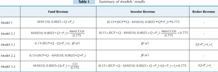
In this section, we compare the results obtained by the models. Table 1 shows the revenue received by each player in the Nash equilibriums of the models developed here.
* *
* *
* *
* *
* *
* *
Table 1 Summary of models' results
Fund Revenue Investor Revenue Broker Revenue
Model 1
-Model 2.1
-Model 3.1
Model 2.2
-Model 3.2
Legend: Model 1: Absence of broker. Model 2.1: Absence of broker. Situation in which the investor owns a minimum amount of stock that allows him/her to renegotiate his/her contract with the funds. ( ). Model 2.2: Absence of broker. Situation in which the investor does not own a minimum amount of stock that allows him/her to renegotiate his/her contract with the funds. ( ). Model 3.1: Presence of broker. Situation in which the amount of stock in the investor’s custody does not allow him/her to renegotiate his/her contract with the funds because the broker’s incremental cost renders the renegotiation unfeasible.(Q P-1 Ic - CT - CTI > CT). Model 3.2: Presence of broker. Situation in which the amount of stock in the investor's custody allows him or her to renegotiate his/her contract with the fund (Q P-1 Ic - CT - CTI > CT).
MAX {10; 0.0025 *Q P* -1} (0.15 *JSCP *Q - MAX{10; 0.0025 *Q P* -1}) 0.775 *
(0.15 *JSCP Q - MAX{10; 0.0025 *Q P* -1}- 0.775Min(CO,0)* 0.775
*
MAX{10; 0.0025 *Q P* -1}+Min(CO,0) 0.775
0.15 JSCP Q - (Q P-1) Ic- βf (σ2)
* * * * βf (σ2)
βf (σ2)
(Q P* -1) I*c
0.15 *JSCP *Q - MAX{10; 0.0025 *Q P* -1}
* *
MAX{10; 0.0025 Q P-1} + CO
0.775 (0.15 *JSCP *Q - MAX{10; 0.0025 *Q P* -1}-(Q P* -1) *Ic) 0.775*
*
+ βf (σ2) + CO + 0.775 MAX {10; 0.0025 Q P
-1}
0.15 0.775 ** *JSCP * Q2 >
*
+ βf (σ2) + CO + 0.775 MAX {10; 0.0025 Q P-1} 0.15 0.775 ** *JSCP * Q2 <
* *
* *
We observe in Table 1 that agents’ revenue is positi-vely affected in all cases by the amount of stock in the custody of the individual investor. This minimum stock amount is also present in the models’ feasibility cons-traints, given that there is generally a minimum stock amount that must be in custody for the lending tran-sactions to be feasible. Therefore, small investors will hardly ever participate in lending transactions like the ones developed in this study. This result corroborates the evidence found by Minozzo (2011) that in Brazil’s market, the type of individual investor who lends his/ her shares is the one with a long-term profile and hi-gher purchasing power. This result also demonstrates that individual investors may extract additional benefit from interest on equity payments, which complements the results by Colombo and Terra (2012), who had al-ready pointed out the benefits obtained by institutio-nal investors when receiving proceeds via interest on equity.
Furthermore, the lower the investor’s opportuni-ty cost for offering a new contract in the absence of a broker, the higher his/her revenue and therefore the higher the investment fund’s revenue. In extreme ca-ses in which the investor’s opportunity cost of offering a new contract to the fund is zero, we have the same equilibrium as for model 1, in which the fund’s revenue covers only the lending transaction’s registration costs. However, in those cases in which the investor’s oppor-tunity cost is extremely high, the investment fund will retain the largest part of the transaction’s revenue and, in extreme cases, the investor’s revenue will be suffi-cient only to cover his or her risk aversion. Thus, we demonstrate that there will be cases in which the fund can extract a large part of the gain and the investor loses his or her bargaining power. Such situation pro-vides an additional reason to conduct stock lending transactions, aside from the possibility of gains for the investor, even if such tax arbitration does not benefit the stock market in terms of an increase in asset value, as shown by Fraga (2013).
The results show that in the simpler case of model 1, the investor always extracts the entire tax gain realized by the lending transactions, deducting the costs incur-red by the fund. This result is intuitive because in this case, neither player has transaction costs. However, in models 2 and 3, the investor can no longer extract the lending transaction’s entire profit. In the former case, this is due to high transaction costs and in the latter case, it is due to the presence of a broker and the resul-ting limitations.
In model 2, the fact that there is a cost for the investor when offering a new contract may require that:
Here, Q2 is the minimum amount of stock that the in-vestor must own to make the contract renegotiation. In this case, the investor accepts any contract offered that remu-nerates his/her risk aversion and therefore, the fund’s reve-nue is the entire tax gain minus the investor’s risk aversion payment.
The constraints derived in model 2 regarding the mini-mum amount of stock that the investor must own for the contract to be signed are given by:
when the minimum lending transactions registration fee does not exceed R$10.00, and
otherwise.
In model 3, the introduction of the broker brings an additional constraint to the game, considering that all of the constraints in model 2 have been met. In this
+ βf (σ2) + CO + 0.775 MAX {10; 0.0025 Q P
-1}
0.15 0.775 JSCP
* * *
* * Q2 <
+ βf (σ2) + CO + 7.75 0.775 (0.15 JSCP) Q2 >
βf (σ2) + CO
0.775 (0.15 JSCP - 0.0025 P-1) Q2 >
case, the presence of the broker can render some con-tracts unfeasible that previously were not. Notice also that model 3 implies that the broker only offers the contract proposed by the fund to those clients that own a minimum stock amount, due to the costs and spread fee charged by the broker.
Therefore, it should be noted that, in some situations, one might find Q3≠Q2 In these cases, contracts that the funds previously offered directly to the investors, who accepted them, are no longer viable once brokers appear. Part of this problem results from the fact that brokers in Brazil do not operate in perfect competition. If they did operate in perfect competition (assuming brokers with
Q3 > CT
P-1 *Ic
costs equal to CT, brokers would no longer choose the spread to be charged in the lending transaction, but would instead calculate the fee to be charged to cover their costs by observing the amount of stock in their clients’ custo-dy. As a result, more contracts would be signed, given that the decision of how much to charge the client would become endogenous to cover only the broker’s marginal costs (assuming that in the perfect competition market, the broker’s cost structure is maintained). Finally, inde-pendent of the hypothesis on competition, it is still reaso-nable to consider that CT+CO2<CO, i.e., that the investor’s cost of offering a new contract is lower when the broker is present, implying that the broker’s presence would increa-se market efficiency by reducing transaction costs. There-fore, the broker’s presence would cause more contracts to be accepted because there would be an overall reduction in costs.
6 CONCLUSION
In this article, we have studied a lending transaction structured via stock lending on the eve of the interest on equity payment, motivated by the possibility of po-sitive gains due to the difference in tax rules applica-ble to the parties involved, namely individual investor and investment fund. In this case, investment funds are exempt from income taxes on interest on equity, whereas individual investors are subject to a tax rate of 15%. Due to the possibility of tax arbitration that arises from this difference, our study develops three theoreti-cal models that seek to explain how the tax gain is split among investors, investment funds and brokers.
In the first model, we have a situation in which the-re athe-re no transaction costs for either investors or funds, and there is no intermediary institution (broker). In the second model, we assume that the investor incurs some costs from offering new contracts, which repre-sent all possible costs for him/her. Finally, in model 3, we include an intermediary institution. By comparing results, we arrived at the conclusion that more contracts (or at most the same number of contracts) are signed in the case in which the broker does not intermediate because under certain conditions, the presence of the brokerage agent imposes additional transaction costs on the model.
In all models, we have observed that not all indi-vidual investors will have an incentive to lend their stock. We have observed that the feasibility of lending transactions depends on the existence of a minimum amount of stock. Therefore, only investors with a long-term profile have an incentive to participate in stock-lending transactions aimed at exploiting the opportu-nity for additional gain that comes with the difference in tax rules for receiving interest on equity, which rein-forces the results of Minozzo (2011).
With respect to the investment fund’s incentive, we have shown that there may be situations, depending on the investor’s cost of offering new contracts, in
whi-ch the fund can extract the largest part of the lending transaction’s revenue. In this way, it is possible for the investor to lose his/her bargaining power. On the other hand, an interesting additional result is that in the pre-sence of a broker, the fund’s profit is reduced because the broker’s presence reduces the investor’s cost of offe-ring a new contract.
Finally, we have found that there is a trade off re-garding the presence of intermediary brokerage insti-tutions in the lending transactions. When intermediary institutions are absent, investors’ costs for offering new contracts are higher; however, brokers impose additio-nal constraints on the problem because of the spread that they charge. Even when brokers operate in perfect competition, given the model’s design there are still ca-ses in which contracts that would be possible in their absence are not affected. However, the broker’s presen-ce causes a large reduction in the lending transaction’s “communication costs”, leading to potentially better equilibriums for the investor.
Boulton, T. J., Braga-Alves, M. V., & Shastri, K. (2012). Payout policy in Brazil: dividends versus interest on equity. Journal of Corporate Finance, 18 (4), 968-979.
Brito, R. D., Lima, M. R., & Silva, J. C. (2009). O crescimento da
remuneração direta aos acionistas no Brasil: economia de impostos ou mudança de características das irmas? BBR Brazilian Business Review, 6 (1), 62-81.
Colombo, J. A., & Terra, P. R. S. (2012). Juros sobre o capital próprio, estrutura e propriedade e destruição de valor: evidências no Brasil.
Anais do Encontro Nacional de Economia, Porto de Galinhas, BA, Brasil, 40.
Comissão de Valores Mobiliários. CVM. Instrução n. 249, de 11 de abril de 1996. Recuperado em 8 junho, 2012, de http://www.cvm.gov.br/. Comissão de Valores Mobiliários. CVM. Instrução n. 277, de 8 de maio de
1998. Recuperado em 8 junho, 2012, de http://www.cvm.gov.br/. Comissão de Valores Mobiliários. CVM. Instrução n. 441, de 10 de novembro
de 2006. Recuperado em 8 junho, 2012, de http://www.cvm.gov.br/. Comissão de Valores Mobiliários. CVM. Instrução n. 466, de 12 de março
de 2008. Recuperado em 8 junho, 2012, de http://www.cvm.gov.br/. Diamond, D. W., & Verrecchia, R. E. (1987). Constraints on short-selling
and asset price adjustment to private information. Journal of Financial Economics, 18 (2), 277-311.
Dos Santos, A. (2007). Quem está pagando juros sobre capital próprio no Brasil? Revista de Contabilidade e Finanças, 18 (spe), 33-44. Fraga, J. B. (2013). Empréstimo de ações no Brasil. Tese de doutorado,
Escola de Administração de Empresas de São Paulo, Fundação Getúlio Vargas, São Paulo, SP, Brasil.
Fudenberg, D., & Tirole, J. (1991). Game theory. Cambridge: he MIT Press. Futema, M. S., Basso, L. F. C., & Kayo, E. K. (2009). Estrutura de capital,
dividendos e juros sobre o capital próprio: testes no Brasil. Revista Contabilidade & Finanças, 20 (49), 44-62.
Gordon, M. J. (1959). Dividends, earning and stock prices. he Review of Economics and Statistics, 41 (2), 99-105.
Klemm, A. (2007) Allowances for corporate equity. CESifo Economic Studies, 53 (2), 229-262.
Lei n. 9.249, de 26 de dezembro de 1995. Brasil. Recuperado em: 20 julho, 2012, de http://www.receita.fazenda.gov.br/Legislacao/leis/Ant2001/ lei924995.htm.
Lei n. 11.033, de 21 de dezembro de 2004. Brasil. Recuperado em 20 julho, 2012, de http://www.planalto.gov.br/ccivil_03/_ato2004-2006/2004/ lei/l11033.htm.
Levy, H., & Markowitz, H. M. (1979). Approximating expected utility by a function of mean and variance. he American Economic Review, 69
(3), 308-317.
Libonati, J. J., Lagioia, U. C. T., & Maciel, C. V. (2008). Pagamento de juros sobre o capital próprio X distribuição de dividendos pela ótica tributária.
Anais do Congresso Brasileiro de Contabilidade, Gramado, RS, Brasil, 18. Lintner, J. (1956). Distribution of incomes of corporation among
dividends, Retained Earnings, and Taxes. he American Economic Review, 46 (2), 97-113.
Martins, A. I., & Famá, R. (2012). O que revelam os estudos realizados no Brasil sobre política de dividendos? Revista de Administração de Empresas, 52 (1), 24-39.
Miller, M. H., & Modigliani, F. (1961). Dividend policy, growth, and the valuation of shares. Journal of Business, 34 (4), 411-433.
Minozzo, C. A. S. (2011). Determinantes da taxa de aluguel de ações no Brasil. Dissertação de mestrado, Escola de Economia de São Paulo, Fundação Getúlio Vargas, São Paulo, SP, Brasil.
Nash, J. (1950). he bargaining problem. Econometrica, 18 (2), 155-162. Ness Jr, W. L., & Zani, J. (2001). Os juros sobre o capital próprio versus a
vantagem iscal do endividamento. Revista de Administração, 36 (2), 89-102. Receita Federal do Brasil. RFB. (2010). Instrução Normativa n. 1.022, de
5 de abril de 2010. Recuperado em 20 julho, 2012, de http://www. receita.fazenda.gov.br/Legislacao/Ins/2007/in10222010.htm. Rubinstein, A. (1982). Perfect equilibrium in a bargaining model.
Econometrica, 50 (1), 97-110.