Relations Among Technical, Cost and Revenue Efficiencies in Data Envelopment Analysis

Relations Among Technical, Cost and Revenue

Efficiencies in Data Envelopment Analysis

S.M. Mirdehghan

M. Nazaari A.

J. Vakili

Abstract_{—Efficiency is a basic issue in Data}

En-velopment Analysis (DEA). There are different types of efficiency in DEA, e.g. Technical Efficiency (TE), Cost Efficiency (CE) and Revenue Efficiency (RE). They may be different in terms of efficiency score val-ues because they use different information obtained from Decision Making Units (DMUs). One of these efficiency types (TE) uses only input and output quantities, another (CE) uses input, output and in-put cost vectors and still another (RE) uses inin-put, output and output benefit vectors. In real problems, not the cost of each input or the benefit of each out-put is usually known and accessible, and just the costs (benefits) of some inputs (outputs) of each DMU are known. In this paper, we suggest a method and mod-els to measure the efficiency of DMUs when some in-put costs and some outin-put benefits are known. The proposed measure is a generalization of TE, CE and RE. This measure is very useful to evaluate the per-formance of DMUs and uses more information than the other measures. We show that the CCR model to evaluate TE and the minimal cost model to evaluate CE are special cases of the proposed model. Finally we present three examples to compare the proposed measure of efficiency with the other measures of effi-ciency.

Keywords: Data Envelopment Analysis, Technical effi-ciency, Cost effieffi-ciency, Revenue efficiency.

1

Introduction

Data Envelopment Analysis (DEA) is a mathematical method that measures the relative efficiency of a group of Decision Making Units (DMUs) with multiple inputs and outputs but with no obvious production function to aggregate the data in its entirety. Debreu (1951) pro-vided the first measure of efficiency and Koopmans (1957) was the first to define the concept of Technical Efficiency (TE). The measurement of TE as defined by Farrell

∗_{Corresponding author.}

a: Department of Mathematics, College of Sciences, Shiraz Univer-sity, Shiraz, Iran

b: Department of Mathematics, Payame Noor University, Tehran Iran

c: Faculty of Mathematical Sciences, Tabriz University, Tabriz, Iran.

Email Adresses: mirdehghan@shirazu.ac.ir (S.M. Mirdehghan), m.nazari@pnu.ac.ir (M. Nazaari A.), j.vakili@tabrizu.ac.ir (J. Vak-ili).

(1957) was operationalized and popularized by Charnes et al. (1978), which led to the establishment of DEA as a prominent methodological tool for assessing relative efficiency. The standard DEA method measures TE as-suming Constant Returns to Scale (CRS) which was ini-tially proposed by Charnes, Cooper and Rhodes (CCR) (1978). Some of DEA researchers worked on the the-ories of DEA and found some characterizations of DEA models. Fukuyama (2000), Sueyoshi and Sekitani (2007), Jahanshahloo et al. (2008) and (2009) found some prop-erties in DEA to find returns to scale, reference set and strong defining hyperplanes. On the other hand, some of the other researchers in different fields and majors ap-plied DEA models to evaluate commerical firms, hospi-tals and etc; see for example Ayaz and Alptekin (2012), Karadayi and Karsak (2014) and Yang (2009). In eval-uating a DMU sometimes the optimal solution(s) of the traditional models is far from the expected results. To solve this shortcoming, the weight restrictions have been added to the traditional models regarding the manage-ment decision. Podinovski (2004) and (2007) and Podi-novski and Thanassoulis (2007) presented some theories of the weight restriction methods.

Cost Efficiency (CE) evaluates the ability of a DMU to produce the current output at minimal cost, given its in-put prices. The concept of CE can be traced back to Farrell (1957), who originated many of the ideas under-lying efficiency assessment. CE can be interpreted as an achievable measure of potential cost reduction given the outputs produced and current input prices at each DMU. The Farrell concept was developed by F¨are et al. (1985), who formulated a Linear Programming (LP) model for CE assessment. This LP model requires input and out-put quantity data as well as inout-put prices at each DMU. Jahanshahloo et al. (2008) simplified a version of the cost efficiency model proposed by Camanho and Dyson (2005) which they showed that the measure of CE can be obtained with the inclusion of weight restrictions in DEA models.

on the performance of a DMU. But providing a more precise, quantitative measure reflecting such a factor is generally beyond the realm of reality. In some situations, such factors can be legitimately ’quantified’, but very of-ten such quantification may be superficially forced as a modeling convenience.

In this paper we propose a model for evaluating the mea-sure of efficiency when some input prices and some output benefits are available for all DMUs. We notate this pro-posed efficiency measure by PE, and we show that the multiplier form model, the minimal cost model and the maximal revenue model for evaluating TE, CE and Rev-enue Efficiency (RE), respectively, are special cases of our proposed model. This means TE (by using CCR model), CE and RE are special measures of PE. This method is completely different from the existing weight restriction methods. The structure of this paper is as follows: Sec-tion 2 describes the DEA models used for the estimaSec-tion of TE, Farrell-Debreu and Tone CE and RE. Some def-initions and models in are extracted from Cooper et al. (2007). In Section 3 we propose a model for evaluat-ing PE. Also, in this section we prove that the minimal cost model for evaluating CE is a special case of the pro-posed model. Section 4 contains three examples to apply the proposed model and compare PE with the other mea-sures of efficiency. Conclusions and suggestions for future research are presented in Section 5.

2

Background

2.1 Technical Efficiency

Relative efficiency is defined as the ratio of the total weighted output to the total weighted input. Suppose that we havenDMUs with activity vectors (xt

j,ytj); j=

1,2, . . . , n,wherexjandyjare nonnegative and nonzero

column vectors in Rm _{and R}s_{, respectively. All DMUs}

(DM Uj (j = 1, . . . , n)) use the same number, m, of

in-puts (xij (i = 1, . . . , m)) to produce the same number,

s, of outputs (yrj (r = 1, . . . , s)). Note that the input

and output vectors of all DMUs are the same in type but different in quantity.

Let

sbe the number of outputs;

mbe the number of inputs;

n be the number of DMUs whose performance must be

evaluated;

yrj be the value (≥ 0) of outputr (r = 1,2, . . . , s) for

DMUj (j= 1,2, . . . , n);

xij be the value (≥ 0) of input i (i = 1,2, . . . , m) for

DMUj (j= 1,2, . . . , n);

uro be the weight (≥ 0) attached to output r (r =

1,2, . . . , s) by DMUo(o∈ {1,2, . . . , n});

vio be the weight (≥ 0) attached to input i (i =

1,2, . . . , m) by DMUo (o∈ {1,2, . . . , n});

θ∗

obe the (relative) efficiency of DMUo(o∈ {1,2, . . . , n});

εbe a very small non-Archimedean number, smaller than any positive real number (0< ε≪1).

The fractional model to evaluate the relative efficiency of

DM Uo(o∈J ={1,2, . . . , n}) is as follows:

θ∗

o = max

s

r=1uroyro/

m

i=1vioxio

max{s

r=1uroyrj/

m

i=1vioxij:j∈J}

s.t. uro≥0; r= 1,2, . . . , s

vio≥0; i= 1,2, . . . , m.

(1)

The measure of relative efficiency of DM Uo is θo∗;

note that 0 ≤ θ∗

o ≤ 1 (and θ∗o = 0 if and only if

yro = 0 (r = 1,2, . . . , s)). The result of the DEA is

the determination of the hyperplanes that define an envelope surface or Pareto frontier. DMUs that lie on the envelope surface are deemed efficient, whilst those that do not are deemed inefficient. By Charnes-Cooper transformations, the fractional model is transformed to the following LP:

max s_r=1uroyro

s.t. m_i=1vioxio= 1

s

r=1uroyrj−

m

i=1vioxij≤0; j= 1,2, . . . , n

uro≥0; r= 1,2, . . . , s

vio≥0; i= 1,2, . . . , m.

(2) Model (2) is called the ”input-oriented” multiplier form to evaluate the relative efficiency ofDM Uo. It is assumed

that the production function exhibits constant returns to scale. The dual of (2) is

min θ

s.t. n_j=1λjxij+s

−

i =θxio; i= 1,2, . . . , m

n

j=1λjyrj−s +

r =yro; r= 1,2, . . . , s

λj≥0; j= 1,2, . . . , n

s−i ≥0; i= 1,2, . . . , m

s+

r ≥0; r= 1,2, . . . , s

θ is unrestricted.

(3)

Model (3) is called the ”input-oriented” envelopment form to evaluate the relative efficiency of DM Uo. We

know that the optimal value of Models (2) and (3) are equal. In the above model s−_i (i = 1,2. . . . , m) are the input excesses and s+

r (r = 1,2. . . . , s) are the output

shortfalls.

Definition 1 DM Uo is called technical efficient if the

Technical efficiency is also referred to as radial efficiency. Technical efficient DMUs are classified in two types; strong efficient DMUs and weak efficient DMUs. In eval-uating DMUo, which is a technical efficient DMU, by (3)

if all slacks s−_i and s+

r (i = 1, ..., m, r = 1, ..., s) equal

zero in all possible optimal solutions then DMUois called

a strong efficient DMU otherwise, it is called a weak effi-cient DMU.

If a DMU proves to be inefficient, a combination of other efficient units can produce either greater outputs for the same composite of inputs or produce the same outputs for a smaller composite of inputs. Similarly, the ”output-oriented” envelopment form and the ”output-”output-oriented” multiplier form are as follows:

φ∗

o= max φ

s.t. n_j=1λjxij+s

−

i =xio; ∀i

n

j=1λjyrj−s +

r =φyro; ∀r

λj≥0; ∀j

s−_i ≥0; ∀i

s+

r ≥0; ∀r

φ is unrestricted.

(4)

min sr=1vixio

s.t. s_r=1uryro= 1

s

r=1uryrj−

m

i=1vixij≤0; ∀j

ur ≥0; ∀r

vi≥0; ∀i.

(5)

We know thatθ∗

o=

1

φ∗

o, whereφ

∗

o is the optimal value of

(4).

2.2 Cost Efficiency

Cost efficiency evaluates the ability of a DMU to pro-duce the current outputs at minimal cost, given its input prices. Looking beyond TE, Farrell (1957) also proposed a measure of cost efficiency, which assumes that prices are fixed and known and maybe different among DMUs. Suppose that there exist nDMUs as defined in 2.1, and

cij≥0 is the cost of theith input ofDM Uj which may

vary from one DMU to another. The minimal cost model to produce at least the current output of DM Uo (yo)

yields the optimal value of the following LP (m_i=1ciox

∗

i).

CEo= m 1 i=1cioxio

min mi=1cioxi

s.t. n_j=1λjxij≤xi; ∀i

n

j=1λjyrj≥yro; ∀r

λj≥0; ∀j

xi≥0; ∀i.

(6)

Because the cost of inputs are nonnegative for each DMU, there exists an optimal solution such as (λ∗t

,x∗t

) such that all constraints (n_j=1λjxij≤xi) are binding. This means the optimal value of (6) equals the optimal value

of the following LP:

CEo= m 1 i=1cioxio

min m_i=1cioxi

s.t. nj=1λjxij=xi; ∀i

n

j=1λjyrj≥yro; ∀r

λj≥0; ∀j

xi≥0; ∀i.

(7)

CEo is the cost efficiency ofDM Uo and it is clear that

CEo ≤ 1. Also this cost efficiency measure is named

Farrell-Debreu cost efficiency measure.

Tone(2002) found an unacceptable property of the traditional Farrell-Debreu cost efficiency measure when the unit prices of input are not identical among DMUs. He suggested a new approach to measure the cost efficiency which we call Tone Cost Efficiency (TCE). TCE is obtained from the following model:

T CEo= m1 i=1xio

min m_i=1xi

s.t. n_j=1λjxij≤xi; ∀i

n

j=1λjyrj≥yro; ∀r

λj≥0; ∀j

xi≥0; ∀i.

(8)

Wherexij=cijxijandxiare variables (i= 1, ..., m, j=

1, ..., n).

The difference between Farrell-Debreu cost model and Tone model is: in the Farrell-Debreu model, the unit cost of DMUo is fixed atco and then the optimal input

vector x∗ _{that produces the output vector y}

o is found,

while, in Tone cost model, the optimal input vector x∗

is searched which can produceyo.

2.3 Revenue Efficiency

Revenue efficiency evaluates the ability of a DMU to pro-duce outputs at maximal revenue when it consumes the current inputs. Suppose that there existnDMUs as de-fined in 2.1, and brj≥0 is the benefit of therth output

of DM Uj. The maximal revenue model to consume at

most the current input ofDM Uo (xo) gives the optimal

value of the following LP (s_r=1broy∗r).

max sr=1broyr

s.t. n_j=1λjxij≤xio; ∀i

n

j=1λjyrj≥yr; ∀r

λj≥0; ∀j

yr ≥0; ∀r.

(9)

Based on an optimal solutiony∗t= (y∗

1, y∗2, . . . , ys∗) of this

model, the revenue efficiency of DM Uois defined as:

REo=

s

r=1broyro s

r=1broyr∗

(10)

In Cooper et al. (2006) ’s a similar discussion to Tone cost model, which has been presented in 2.2, has been presented for the revenue efficiency.

3

The Proposed Efficiency Measure

In this section, we propose a model to evaluate efficiency when some (not necessarily all) elements of the input cost vector and some (not necessarily all) elements of the out-put benefit vector are available. We consider the frac-tional multiplier form model (1) to obtain the proposed model.

Suppose that there exist n DMUs, namely

DM U1, DM U2, . . . , DM Un where DM Uj; j =

1,2, . . . , n has the input vector xj with m elements

and the output vectoryj withselements.

We form the virtual input and output by weights (vi)

and (ur) (yet unknown) as follows:

virtual input=v1x1o+v2x2o+. . .+vmxmo,

virtual output=u1y1o+u2y2o+. . .+usyso.

Then, we try to determine the weights, using linear pro-gramming so as to maximize the ratio

virtual output virtual input.

The optimal weights may (and generally will) vary from one DMU to another. Thus, the weights in DEA are derived from the data rather than being fixed in advance. A best set of weights is assigned to each DMU with values that may vary from one DMU to another.

Let J = {1,2, . . . , n}. To evaluate the efficiency mea-sure ofDM Uo (o∈ {1,2, . . . , n}), we solve the following

fractional programming model to obtain values for the in-put weights (vi; i= 1,2, . . . , m) and the output weights

(ur;r= 1,2, . . . , s) as variables:

max θ=

u1y1o+u2y2o+...+usyso v1x1o+v2x2o+...+vmxmo

max{u1y1j+u2y2j+...+usysj v1x1j+v2x2j+...+_vmxmj:j∈J}

s.t. ur≥0; r= 1,2, . . . , s

vi≥0; i= 1,2, . . . , m.

(11)

The objective is to obtain weights (vi) and (ur) that

max-imize the ratioθof DMUoas the DMU under assessment.

According to the objective function, the optimal objective valueθ∗_{is at most 1. Mathematically, the nonnegativity}

constraints are not sufficient for the fractional terms in the objective function to have a definite value. We do not consider this assumption in explicit mathematical form at this time. Instead, we put this in managerial terms by assuming that all outputs and inputs have some nonzero values and this is to be reflected in the weightsur andvi

being assigned some positive values.

According to the above discussion, Model (11) obtains the best weights for inputs and outputs to maximize the objective function. On the other hands in real prob-lems we may have the real value of some input prices and some output benefits, while Model (11) ignores this fact and so the efficiency obtained from this model is un-acceptable because the optimal weights given by Model (11) may be different from the real weights (the market prices) that are available. Also, the optimal weights of (11) are the same for all DMUs in evaluating the DMU under assessment. For example, in assessing DMUo, if

(v∗

1, v∗2, . . . , vm∗, u∗1, u∗2, . . . , u∗s) is an optimal weight

vec-tor of (11), v∗

i is the weight (shadow price) of the ith

input of all DMUs while in real problems the ith inputs may be different in price in each DMU.

Suppose that there exist n DMUs

(DM U1, DM U2, . . . , DM Un) with activity

vec-tors D1,D2, . . . ,Dn where Dj = (xtj,yjt);

xt_j = (x1j, x2j, . . . , xmj) and ytj = (y1j, y2j, . . . , ysj).

Furthermore, some input prices and some output benefits are available. Without loss of generality, suppose that the input prices of the first p (p ≤ m) elements of each input vector and the output benefits of the first

q (q ≤ s) elements of each output vector are available. Let vt_j = (v1j, v2j, . . . , vpj), utj = (u1j, u2j, . . . , uqj),

vt = (vp+1, vp+2, . . . , vm) and ut = (uq+1, uq+2. . . , us)

where vij;i= 1,2, . . . , p, is theith input cost ofDM Uj

and urj;r = 1,2, . . . , q, is the rth output benefit of

DM Uj. Note that input cost vectors (vtj) and output

benefit vectors (utj) may be different for each DMU.

To obtain the proposed efficiency ofDM Uoconsider the

following model:

θ1= max

u1o y1o+...+uqoyqo+_uq+1yq+1o+...+usyso v1o x1o+...+vpoxpo+_vp+1xp+1o+...+vmxmo

max{ u1j y1j+...+_{uqj yqj}+_uq+1yq+1j+...+_usysj

v1j x1j+...+_{vpj xpj}+_vp+1xp+1j+...+_vmxmj:j∈J}

s.t. ur ≥0; r=q+ 1, q+ 2, . . . , s

vi≥0; i=p+ 1, p+ 2, . . . , m,

(12) whereur (r=q+ 1, . . . , s) andvi(i=p+ 1, . . . , m) are

variables andurj, vij(r= 1,2, . . . , q, i= 1,2, . . . , p, j=

1,2, . . . , n) are constants. We assume that v1jx1j +

v2jx2j +. . .+vpjxpj +vp+1xp+1j +vp+2xp+2j +. . .+

vmxmj = 0 for all j. Let xjt = (x1j, x2j, . . . , xpj),

xt_j = (xp+1j, xp+2j, . . . , xmj),ytj= (y1j, y2j, . . . , yqj) and

y_jt= (yq+1j, yq+2j, . . . , ysj).

Any two vectors vt_j, xj can be multiplied. The result

of this multiplication is a real number called the inner product of the two vectors, which is defined as:

vt_jxj=v1jx1j+v2jx2j+. . .+vpjxpj.

Let kj = vtjxj, wj = utjyj and z = 1

max{wj+utyj kj+vtxj

:j∈J}

Model (12) is transformed to the following model:

max woz+utyoz

ko+vtxo

s.t. wjz+utyjz

kj+vtxj ≤1; j∈J

u≥0 v≥0

z≥ε.

(13)

To transform Model (13) to a linear programming

problem, let t= 1

ko+vtxo and use the following variables

changes:

uttz−→ut vtt−→vt

zt−→z.

Note that variables z and t are greater than zero. Model (13) is transformed as follows:

θ2= max woz+utyo

s.t. kot+vtxo= 1,

wjz+utyj−(kjt+vtxj)≤0; j∈J

t≥ε, u≥0

z≥ε, v≥0

(14) whereεis a non-archimedean number. The above model is called the ”Input-oriented multiplier proposed model.”

Remark: The proposed method is completely dif-ferent from the existing weight restriction methods. In the DEA literature some weight restrictions have been

added to some DEA models. In evaluating a DMU

by the DEA models (without any weight restriction) the corresponding weights to an input/output for all

DMUs are the same. For example to assess DMUo,

the first input (output) of all observed DMUs have the same unknown weights and, in our notation it has been presented by v1 (u1). While the proposed method assigns the actual market price as a weight to each input and output which their market prices are available, and assigns the unknown weights to each input and output as variables which their market prices are not available.

Theorem 1 The optimal values of (12) and (14) are equal.

Proof: Suppose that (u∗t

,v∗t

) is an optimal solution of (12). Lett∗₌ 1

ko+v∗t_xo andz

∗_=t∗_/max{wj+u∗

t

yj kj+v∗t_xj :j∈ J} then (ut_,vt_{, t, z) = (z}∗_u∗t

, t∗_v∗t

, t∗_{, z}∗_{) is a feasible}

solution of (14), so

θ2≥woz∗+u∗ t

z∗yo=θ1. (15)

Also, suppose that (u∗t

,v∗t

, t∗_{, z}∗_{) is an optimal}

so-lution of (14), then (ut_,vt_{) = (}u∗

t z∗ ,

v∗

t

t∗ ) is a feasi-ble solution of (12). Moreover, because (u∗t

,v∗t

, t∗_{, z}∗₎

is a feasible solution of (14), kot∗ + v∗ t

xo = 1 and

wjz∗+u∗ t

yj−(kjt∗+v∗ t

xj)≤0 for allj∈J. Therefore

max{wjz∗+u∗

t

yj

kjt∗+v∗t_xj :j∈J} ≤1.So θ1≥[(wo+u

∗t

z∗ yo)/(ko+

v∗

t

t∗ xo)]/max{(wj+

u∗

t

z∗ yj)/(kj+

v∗

t

t∗ xj) : j ∈ J} = [(woz

∗ _{+ u}∗t

yo)/(kot∗ +

v∗t

xo)]/max{(wjz∗+u∗ t

yj)/(kjt∗+v∗ t

xj) :j∈J} ≥

woz∗+u∗ t

yo=θ2.

From (15) and the above relation, we have θ1= θ2 and the proof is completed.

The proof of this theorem shows that if (u∗t

,v∗t, t∗_{, z}∗_{) is}

an optimal solution of (14), then (u∗

t z∗ ,

v∗

t

t∗ ) is an optimal solution of (12), and one of the best weight vectors for the inputs and outputs ofDM Uo, which their market prices

are not available, is (u∗

t z∗ ,

v∗

t t∗ ).

The dual of (14) is called the ”input-oriented envelopment proposed model” and is shown below:

min θ−ε(s+_+s−₎

s.t. nj=1λjxij ≤θxio; i=p+ 1, . . . , m

n

j=1λjkj+s

−_=θk

o

n

j=1λjyrj≥yro; r=q+ 1, . . . , s

n

j=1λjwj−s +_=w

o

λj≥0; j∈J

s+_≥0

s−_≥0

θ is unrestricted.

(16)

Because of the non-Archimedean number ε, we solve the following problems to find the optimal solution of (16).

min θ

s.t. n_j=1λjxij≤θxio; i=p+ 1, . . . , m

n

j=1λjkj≤θko

n

j=1λjyrj≥yro; r=q+ 1, . . . , s

n

j=1λjwj≥wo

λj≥0; j∈J

θ is unrestricted.

(17)

Using our knowledge of θ∗, the optimal value of (17), we solve the following LP usingλ, s+ _ands−_{as variables:}

max s+_+s− s.t. n_j=1λjxij ≤θ

∗_x

io; i=p+ 1, . . . , m

n

j=1λjkj+s

−_=θ∗_k

o

n

j=1λjyrj≥yro; r=q+ 1, . . . , s

n

j=1λjwj−s +

=wo

λj≥0; j∈J

s+

≥0

s−_≥0

It is easy to show that θ∗ _{is the optimal value of (17)}

and (λ∗t

, s+∗_{, s}−∗_{) is an optimal solution of (18) if and}

only if (λ∗t

, θ∗_{, s}+∗_{, s}−∗_{) is an optimal solution of (16).}

Suppose that (λ∗t

, θ∗_{, s}+∗_{, s}−∗_{) is an optimal solution of}

(16). Consider the following virtual DMU

(

n

j=1

λ∗

jxtj, n

j=1

λ∗

jytj)

1. For the first p inputs whose weights (market prices) are known, the total cost (n_j=1λ

∗

jkj) is contracted with

respect toko, and

2. for the last m− p inputs, whose weights are un-known, the virtual inputs are contracted with respect to

xo. These mean that the firstpinputs and the lastm−p

inputs of the virtual DMU are contracted with respect to in cost and quantity, respectively, by a contraction factor

θ∗_.

(λt, θ, s+

, s−_{), in whichλ}

o= 1,λj= 0 (j∈J andj=o),

θ= 1, s+_{= 0 ands}− _{= 0, is a feasible solution of (16).}

Also if mi=p+1xio+ko = 0, then the optimal value of (16) is bounded. By the duality theorem the dual of (16), i.e. (14), is feasible.

Definition 2 DM Uo is efficient if and only if the

op-timal value of (17) equals one and the opop-timal value of (18) equals zero otherwise, it is inefficient.

In a similar way we can show that the ”output-oriented multiplier proposed model” and the ”output-oriented en-velopment proposed model” are as follows:

min kot+vtxo

s.t. woz+utyo= 1

wjz+utyj−(kjt+vtxj)≤0; j∈J

t≥ε, u≥0

z≥ε, v≥0

(19)

max φ+ε(s+_+s−₎ s.t. n_j=1λjxj ≤xo

n

j=1λjkj+s−=ko

n

j=1λjyj ≥φyo

n

j=1λjwj−s +_=φw

o

λj≥0; j∈J

s+_≥0

s−_≥0

φ is unrestricted.

(20)

Theorem 2 φ= 1

θ∗, where ’∗’ and ’∼’ indicate the

op-timality of (16) and (20), respectively.

Proof: Suppose that (λ∗t

, θ∗_{, s}+∗_{, s}−∗_{) and}

(λt_{,φ, s}+_,s−_{) are the optimal solutions of (16) and}

(20), respectively. (λt_{, φ, s}+_{, s}−_{) = (}λ∗t

θ∗ , 1

θ∗,

s+∗

θ∗ ,

s−∗

θ∗ ) is a feasible solution of (21), therefore φ+ε(s+_+s−_{) ≥}

1

θ∗ +

ε θ∗(s

+∗_+s−∗_{). So}

1−φθ ∗≤ε[θ∗(s+_+s−_)−(s+∗_+s−∗_{)]. (21)}

Also (λt_{, θ, s}+_{, s}−_{) = (}λt

φ,

1

φ,

s+

φ,

s−

φ) is a feasible solution

of (16), soθ∗_−ε(s+∗_+s−∗_)≤ 1

φ− ε

φ(s

+_+s−_{). It implies}

1−φθ ∗≥ε[(s+_+s−_)−φ(s+∗_+s−∗_{)]. (22)}

Sinceεis a non-Archimedean number, then (21) and (22) show thatφθ ∗_{= 1.}

Consider Model (14). If all input prices and output ben-efits are unknown or we do not use input cost and output benefit information in Model (14), then parameters wj

andkjfor alljand variableszandtare omitted.

There-fore, what remains of Model (14) is the ”input-oriented multiplier CCR model” and its optimal value is TE.

Here we show that the minimal cost model (7) for eval-uating cost efficiency is a special case of our proposed model; that is, the optimal value of our proposed model when all input prices are available and all output benefits are unknown is the cost efficiency measure ofDM Uo.

Consider the proposed model to evaluate DM Uo when

all input prices are available and all output benefits are unknown. In evaluating the measure of PE for DMUo, we

assume that the input cost vectors of all DMUs are the same and equal toco_{, the input cost vector ofDM U}

o. In

this case, the proposed model is converted to:

max utyo

s.t. cotxot= 1

utyj−co t

xjt≤0; j= 1,2, . . . , n

u≥0

t≥ε.

(23)

In the above modelcotxo>0 andt= 1

cotxo. By setting

the value oftin the other constraints, the modified model is:

max utyo

s.t. utyj≤ c ot

xj

cotxo; j= 1,2, . . . , n

u≥0

(24)

The dual of the above model is:

min cot

cotxo

n

j=1λjxj

s.t. n_j=1λjyj≥yo

λj≥0; j= 1, . . . , n.

(25)

Let x=n_j=1λjxj, so the above model is equal to:

min cotx cotxo

s.t. n_j=1λjxj =x

n

j=1λjyj ≥yo

λj≥0; j= 1, . . . , n.

whereλj (j= 1, . . . , n) andxare variables.

The preceding model is the ”Cost Model” to evaluate

DM Uo, and its optimal value is the cost efficiency

mea-sure of DM Uo. A similar process can be used to prove

that PE is equal to TCE. In this casekj=cjxjand,vtxj

and wjz will be removed from (14).

Furthermore, the model for measuring the revenue effi-ciency is a special case of the model for evaluating PE when all output benefits are available, and by using the ”output-oriented multiplier proposed model” the proof is similar to the above.

4

Examples

Example 1

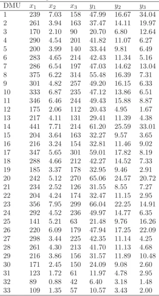
Kim et al. (1999) examined 33 telephone offices, each having 3 inputs and 5 outputs, in Korea. We select 3 in-puts and 3 outin-puts from among their data for evaluating the DMUs. All inputs and outputs are quantitative. We use the following factors:

Inputs

(x1) :Manpower. the number of regular employees.

(x2) : operating costs. Various costs except for interest cost (million dollars).

(x3) :number of telephone lines. Outputs

(y1) :local revenues. The total revenues of local telephone services in each office (million dollars).

(y2) :long distance revenues. The total revenues of long-distance telephone services in each office (million dollars).

(y3) :international revenues. The total revenues of inter-national telephone services in each office (million dollars). Table 1 displays the data.

In this example, outputs 1, 2 and 3 are quantitative and denote the benefits attained from consuming inputs. So, in evaluating DMUs with our proposed model we can use 1,000,000 as weights for outputs 1, 2 and 3.

The DMUs in Table 1 have been evaluated using the pro-posed model (Model (14)). Also, we use the maximal revenue model (Model (9)) and Equation (10) to find the revenue efficiency of DMUs and apply CRS model (Model(3)) to find the technical efficiency, the results of which are presented in Table 2.

We can see that in this example PE and RE of all DMUs are equal because all output benefits are available and equal. This is an example to show that the revenue effi-ciency is a special case of PE. In this example, 6 DMUs are CCR-efficient but the number of the proposed effi-cient DMUs is 4. Also, it can be seen that PE measures

are not greater than CCR efficiency measures.

Note that this result is not true generally (see Example 3).

Table 1

Data for Example 1.

DMU x1 x2 x3 y1 y2 y3

1 239 7.03 158 47.99 16.67 34.04

2 261 3.94 163 37.47 14.11 19.97

3 170 2.10 90 20.70 6.80 12.64

4 290 4.54 201 41.82 11.07 6.27

5 200 3.99 140 33.44 9.81 6.49

6 283 4.65 214 42.43 11.34 5.16

7 286 6.54 197 47.03 14.62 13.04

8 375 6.22 314 55.48 16.39 7.31

9 301 4.82 257 49.20 16.15 6.33

10 333 6.87 235 47.12 13.86 6.51

11 346 6.46 244 49.43 15.88 8.87

12 175 2.06 112 20.43 4.95 1.67

13 217 4.11 131 29.41 11.39 4.38

14 441 7.71 214 61.20 25.59 33.01

15 204 3.64 163 32.27 9.57 3.65

16 216 3.24 154 32.81 11.46 9.02

17 347 5.65 301 59.01 17.82 8.19

18 288 4.66 212 42.27 14.52 7.33

19 185 3.37 178 32.95 9.46 2.91

20 242 5.12 270 65.06 24.57 20.72

21 234 2.52 126 31.55 8.55 7.27

22 204 4.24 174 32.47 11.15 2.95

23 356 7.95 299 66.04 22.25 14.91

24 292 4.52 236 49.97 14.77 6.35

25 141 5.21 63 21.48 9.76 16.26

26 220 6.09 179 47.94 17.25 22.09

27 298 3.44 225 42.35 11.14 4.25

28 261 4.30 213 41.70 11.13 4.68

29 216 3.86 156 31.57 11.89 10.48

30 171 2.45 150 24.09 9.08 2.60

31 123 1.72 61 11.97 4.78 2.95

32 89 0.88 42 6.40 3.18 1.48

Table 2

Results of Example 1.

DMU Technical Revenue Proposed

no Efficiency Efficiency Efficiency

1 1.000 1.000 1.000

2 0.990 0.965 0.965

3 1.000 0.996 0.996

4 0.822 0.668 0.668

5 0.896 0.722 0.722

6 0.792 0.636 0.636

7 0.860 0.714 0.714

8 0.721 0.606 0.606

9 0.803 0.690 0.690

10 0.748 0.577 0.577

11 0.773 0.640 0.640

12 0.780 0.609 0.609

13 0.821 0.666 0.666

14 1.000 1.000 1.000

15 0.788 0.636 0.636

16 0.857 0.810 0.810

17 0.822 0.698 0.698

18 0.794 0.695 0.695

19 0.769 0.624 0.624

20 1.000 1.000 1.000

21 1.000 0.900 0.900

22 0.731 0.587 0.587

23 0.848 0.728 0.728

24 0.872 0.734 0.734

25 1.000 1.000 1.000

26 0.975 0.928 0.928

27 0.969 0.779 0.779

28 0.795 0.776 0.776

29 0.787 0.752 0.752

30 0.774 0.677 0.677

31 0.739 0.658 0.658

32 0.803 0.618 0.618

33 0.720 0.623 0.623

Example 2

Table 3 exhibits four DMUs with two inputs and two outputs, along with the unit cost for each input. The results of evaluating TE, CE and PE are also presented in Table 4.

Table 3

Data of Example 2.

DMU x1 x2 y1 y2 c1 c2

A 2 3 5 8 2 2

B 1 5 2 6 2 4

C 3 8 4 8 3 3

D 2 7 1 2 4 2

Table 4

Results of Example 2.

DMU TE CE TCE PE

A 1.000 1.000 1.000 1.000

B 1.000 0.545 0.341 0.341

C 0.571 0.455 0.303 0.303

D 0.214 0.159 0.114 0.114

According to the results we can see that PE is not equal to CE for DMUsB, C and D because in evaluating PE for each DMU the model uses the corresponding costs for each DMU, but in evaluating the cost efficiency of

DM Uo, the minimal cost model actually uses the input

costs of DM Uo for all other DMUs. This is while the

input costs are practically different in evaluating other DMUs.

In 2.2. we said that Tone cost model has solved the shortcoming of Farrell-Debreu cost model. Regarding Table 4 we see that the results of Farrell-Debreu cost efficiency (CE) are different from TCE. Moreover, we see that the results of PE and TCE are the same. It shows that PE solves the traditional Farrell-Debreu shortcoming too. In general the results of TCE and PE, when we use the inputs and outputs quantities as well as all input prices, are the same.

Example 3.

In this example, we evaluate 12 DMUs with two inputs and two outputs. The unit cost for input 1 and the unit benefit for output 1 are available. The costs and the benefits are different for each DMU. The data are summarized in Table 5.

Table 5

Data for Example 3.

DMUs x1 x2 y1 y2 c1 b1

A 20 151 100 90 500 550

B 19 131 150 50 350 400

C 25 160 160 55 450 480

D 27 168 180 72 600 600

E 22 158 94 66 300 400

F 55 255 230 90 450 430

G 33 235 220 88 500 540

H 31 206 152 80 450 420

I 30 244 190 100 380 350

J 50 268 250 100 410 410

K 53 306 260 147 440 540

L 38 284 250 120 400 295

Table 6

Results of Example 3.

DMU A B C D E F

PE 1.000 1.000 0.894 1.000 1.000 0.719

TE 1.000 1.000 0.883 1.000 0.763 0.835

DMUs G H I J K L

PE 0.942 0.732 0.936 0.765 0.949 0.847

TE 0.902 0.796 0.960 0.871 0.955 0.958

Table 6 shows that there does not exist any relation between TE and PE. For example the PE of DMUs

C, E and G are greater than their TE, while the PE ofF, H, I, J, K andLare less than their TE.

5

Conclusion

There are different types of efficiency measures such as technical efficiency, cost efficiency and revenue efficiency. These measures are different in terms of efficiency score values because each uses different information obtained from decision making units, e.g. technical efficiency only uses the quantities of inputs and outputs; cost efficiency uses the quantities of inputs, outputs and all input prices; and revenue efficiency uses the quantities of inputs, out-puts and all output benefits. But in real problems, some input prices (not necessarily all) and some output ben-efits (not necessarily all) are known. The conventional techniques for measuring efficiency do not use some input prices and some output benefits together. In this paper we proposed a linear programming model to estimate the measure of efficiency when only some input prices and some output benefits are known. This measure is nearer to real world conditions than other measures (TE, CE and RE), because we use real weights in PE while the weights obtained from multiplier forms (used for evalu-ating TE, CE and RE) are possibly different from real weights. The weights obtained from the CCR multiplier form are the best weights to maximize TE. The measures of TE, CE and RE are special cases of PE, and in this paper we showed that TE and CE measures and the cor-responding models are special cases of PE measure and the proposed model, respectively. A shortcoming of the CE measure that our proposed model overcomes is the fact that in evaluating the CE of DMUo it uses the

in-put cost vector of DMUo, i.e. co, for all other DMUs

(see Tone (2002)). Our proposed model uses their corre-sponding input cost vectors for other DMUs. A similar argument can be put forward for RE. PE measure can be used in real worlds problems and it can yield some meth-ods to rank DMUs. The envelopment proposed model to evaluate PE hasn+ 3 variables andm+s+ 2−(p+q) restrictions (except the nonnegativity constraints) while the envelopment form of the CCR model has n+ 1 vari-ables and m+s restrictions (except the nonnegativity constraints). Since our proposed model has fewer con-straints (whenp+q >2) compared to the envelopment form of the CCR model, it seems to be able to evaluate

PE better than the envelopment form of the CCR model in terms of complexity. Using this measure for practi-cal problems and finding some methods to rank DMUs and applying this measure (PE) to other fields of DEA, e.g. ranking, Productivity, returns to scale and etc. are directions for future research.

References

[1] Ayaz, E., Alptekin, S.E.,”Impact of Disinflation on Profitability: A Data Envelopment Analysis

Ap-proach for Turkish Commercial Banks”, Lecture

Notes in Engineering and Computer Science: Pro-ceeding of The World Congress on Engineering 2012,

WCE 2012, 4-6 July, 2012, London, U.K., pp. 447-452.

[2] Camanho, A.S., Dyson, R.G.,”Cost efficiency mea-surement with price uncertainty: A DEA application to bank branch assessments”, European Journal of Operational Research, V161, pp. 432-446, 2005.

[3] Charnes, A., Cooper, W.W., Rhodes, E., ”Measur-ing the efficiency of decision mak”Measur-ing units,” Euro-pean Journal of Operational Research, V2, pp. 429-444, 1978.

[4] Cooper, w.w., Seiford, L.M., Tone, K., ”Data En-velopment Analysis: A Comprehensive Text with Models, Applications, References and DEA-Solver Software,” Second Edition, Kluwer Academic Pub-lishers, 2007.

[5] Debreu, G., ”The coefficient of resource utilisation,”

EconometricaV19, N3, pp. 273-292, 1951.

[6] Fare, R., Grosskopf, S., Lovell, C.A.K., ”The Mea-surement of Efficiency of Production,”Kluwer Aca-demic Publishers, 1985.

[7] Farrell, M.J., ”The measurement of productive ef-ficiency,” Journal of the Royal Statistical Society

V120, pp. 253-281, 1957.

[8] Fukuyama, H., ”Returns to scale and scale elasticity in data envelopment analysis,”European Journal of Operational Research, V125, pp.93-112, 2000.

[9] Jahanshahloo, G.R., Shirzadi, A., Mirdehghan, S.M., ”Finding the reference set of a decision making unit,”Asia-Pacific Journal of Operational Research,

V25, N4, pp. 563-573, 2008.

[10] Jahanshahloo, G.R., Shirzadi, A., Mirdehghan, S.M., ”Finding strong defining hyperplanes of the PPS using multiplier form,” European Journal of Operational ResearchV194, pp. 933-938, 2009.

[11] Jahanshahloo, G.R., Soleimani-damaneh, M.,

[12] Karadayi, M.A., Karsak, E.E., “Imprecise DEA Framework for Evaluating the Efficiency of State Hospitals in Istanbul,” Lecture Notes in Engineer-ing and Computer Science: ProceedEngineer-ing of The World Congress on Engineering 2014, WCE 2014, 2-4 July, 2014, London, U.K., pp. 1018-1023.

[13] Kim, S.H., Park, C.G., Park, K.S., ”An application of Data Envelopment Analysis in telephone offices evaluation with partial data,”Computers and Oper-ations ResearchV26, pp. 59-72, 1999.

[14] Podinovski, V.V., ”Suitability and redundancy of non-homogeneous weight restrictions for measuring the relative efficiency in DEA,”European Journal of Operational ResearchV154, N2, pp. 380-395, 2004.

[15] Podinovski, V.V., ”Computation of efficient tar-gets in DEA models with production trade-offs and weight restrictions,” European Journal of Opera-tional ResearchV181, N2, pp. 586-591, 2007.

[16] Podinovski, V.V., Thanassoulis, E., ”Improving dis-crimination in data envelopment analysis: Some practical suggestions,”Journal of Productivity Anal-ysis,V28, pp. 117-126, 2007.

[17] Sueyoshi, T., Sekitani, K., ”The measurement of re-turns to scale under a simultaneous occurrence of multiple solutions in a reference set and a support-ing hyperplane,” European Journal of Operational ResearchV181, N2, pp. 549-570, 2007.

[18] Tone, K., ”A Strange Case of the Cost and Alloca-tive Efficiencies in DEA,”Journal of the Operational Research SocietyV53, pp. 1225-1231, 2002.