Interval Enclosures for Reliability Metrics
M.A. CAMPOS* and A.F. MENDONC¸ A
Received on October 14, 2015 / Accepted on May 30, 2016
ABSTRACT.The computation of reliability metrics, that arereliability function,mean time to failure, hazard rate function, involves real numbers. Therefore, numerical problems are generated due to the lim-itation of representing and operating with real numbers in computers. This paper is focused on computing intervals that bound numeric errors introduced during computation process of reliability metrics in digital machines for Exponential, Weibull and Normal failure distributions. Interval functions were proposed for controlling numeric errors in the computation of reliability metrics values of complex systems, based on interval mathematics and high accuracy arithmetic. The interval functions calculate interval enclosures, us-ing Intlab toolbox, for real values of reliability metrics and the SHARPE software was used to validate the results. Analysis of the numerical results obtained with the proposed functions showed that the intervals really enclose the real numbers calculated by the SHARPE software, indicating that these functions, in fact, are an alternative for auto-validating representation of these reliability values of complex systems.
Keywords:reliability, interval mathematics, high accuracy arithmetic, interval enclosures.
1 INTRODUCTION
Reliability is defined as the probability that a system (component) will function over some period of time [5]. Usually, it is used for model the system reliability the probability functions: reli-ability functionandhazard rate function. In addition, a common parameter that is usefull in reliability analysis is themean time to failure[5, 13, 23]. Throughout this paper, we call these three ways to quantify reliability aspects asreliability metrics.
As reliability metrics are real numbers, the computation of these values can generate numeric problems caused primarily by the limitation in handling real numbers in a digital machine [6]. The calcutation process introduces round-off and truncation errors [8]. In order to control these types of numeric errors, this paper presents interval functions, which yieldinterval enclosures. These intervals encapsulate guarantee that the real values of reliability metrics, for sure, will be within the computed interval enclosures.
*Corresponding author: Marcilia Andrade Campos.
Let X be the set of all the real numbers x that satisfy X ≤ x ≤ X. Then, X is an interval
[19, 20, 21, 26] with lower and upper bounds equal to X and X, respectively. Thus, X can be give by: X = [X,X] = {x ∈ |X ≤x ≤X}.
We denote the set of the closed real intervals byIIR. Interval functions use arithmetic operations [19, 20, 21] defined onIIR. These interval functions here defined receive as argument a real numbert ≥ 0, which represents the observation time of the system. Therefore, such functions are given byF :R→IIR.
The interval enclosures in this paper have high accuracy [12], i.e., they have the smallest possible width that can be represented in digital machines. High accuracy intervals have lower and upper bounds that belong to the floating-point system of the digital machine [3].
Let be the floating-point systemF ⊆ R. Since X = [X,X] are a high accuracy interval and encloses the real numberx, then (i)X∈F, (ii)X∈F, (iii)X≤x≤ X. These conditions define the called high accuracy intervals [12]. To represent these type of intervals and the arithmetic operations between them in a floating-point system, it is mandatory the use of the directional rounding operators,△(upward direction) and∇(downward direction). Each of these directional operators, when applied to a real numberx, yield a number in the floating-point system closer to x, such that△x∈F,△x≥xand∇x∈F,∇x≤x.
The probabilistic modeling of reliability is based on a nonnegative continuous random variable T, which represents the time to failure of a given system. In this paper, the computed interval encapsulates real values of reliability metrics real values of systems with Exponential, Weibull and Normal time to failure distribution. Analysis were performed using isolated components and complex systems [5] with components logically connected in series and in parallel [13, 23]. These procedures use the Simpson Interval Method [3] to yield interval enclosures for probabil-ity values of continuous random variables [1]. At the end of this work, intervals obtained by the proposed interval functions were compared with the numerical results of the Symbolic Hierar-chical Automated Reliability and Performance Evaluator software (SHARPE) [23]. According to Hirel et al. [9] the SHARPE software is used in the reliability field and performance analysis, being used by universities and companies.
The works of [27, 28, 29, 30] address the same thematic of the current one. These studies present reliability interval analysis aimed to determine failure probabilities with interval parameters. In [4] it is outlined a focus in providing intervals to reliability based on Bayesian analysis. The work of [16] presents interval enclosures for reliability function values of systems with Expo-nential failure distribution. This paper has a new approach that is focused on computing intervals that bound numeric errors introduced during computation process of reliability metrics in digital machines for Exponential, Weibull and Normal failure distributions.
All the computation procedures here presented were performed in the following computational platform:
• Processor: Celeron(R) Dual-Core CPU T3000 1.80 GHz;
• Main Memory: 2.00 GB;
In this paper, the interval computation is performed over the set of IEEE 754 binary64 floating-point numbers [10], which is suitable with the Matlab [15] toolbox Intlab [22]. There are others approaches to implement interval computing, as it is outlined in [7, 11]. We chose IntLab since this toolbox is widely used for users from more than 50 countries. Moreover, Intlab produces reliable results which is proved to be true under any circumstances, in particular covering rouding errors and all error terms [22].
2 RELIABILITY MODELING AND INTERVAL ENCLOSURES
In this section, we define interval functions and their implementations using the IntLab. These interval functions result in interval enclosures for reliability metrics of a system (reliability func-tion, mean time to failure and hazard rate function). Throughout this secfunc-tion, it is considered that the continuous random variableT takes only non-negative values. In this work, calculations are performed forT with Exponential, Weibull and Normal distributions. It is also assumed that this variable can be described by its probability density function fT and cumulative distribution
functionFT. Also, it is assumed that the systems addressed in this paper are not repairable [13].
So, it is not considered repairs and maintenance of any analyzed system.
2.1 Reliability Function
Consider a single component system in operation for the period[0,t]andT its time to failure. The real-valued reliability function of these system, at timet,R(t), is given by:
R(t)=P(T ≥t), (2.1)
whereP(T ≥t)is the probability of the system will not fail during the operation period[0,t].
If fT is the probability density function of the variableT, then
R(t)=
+∞
t
fT(t)dt=1−
t
0
fT(t)dt. (2.2)
In this paper, the interval enclosures for real-valued reliability function are obtained using the Simpson Interval Method [3]. This method is used to calculate intervals that encompass defined integrals over an interval[a,b]of a given real function f. In this method, we divide the integra-tion interval[a,b]in ppartitions whose limits are: a =a0 <a1 <a2 <· · ·<ap =b. This
process of partitioning results in p intervalsAi = [ai−1,ai], wherei =1,2, . . . ,p. For each
partition, one interval enclosure is obtained by
Si =
ai
ai−1
f(t)dt= w(Ai)
6 (F(ai−1)+4f(m(Ai))+F(ai))−
w(Ai)5
2880 G(ξi), (2.3)
wherei =1,2, . . . ,p,ξi ∈ Ai,w(Ai)andm(Ai)are the width and the midpoint ofAi,
This method is employed for calculating the interval Pv([0,t])such that
t
0 fT(t)dt = P(0 < T <t)∈ Pv([0,t]).
As we can see in the Lemma 2.3 of [2], considering Abe a specific probabilistic event, since P(A)=c, thenPv(A)= X = [x1,x2]andc∈ X. InPv([0,t]), we consider that, in this case,
the probabilistic event Aist≥T ≥0.
This work presents implementations intended to compute intervals that encapsulate probabilities of random variables with Exponential, Weibull and Normal distributions [2]. All the developed implementations use Matlab [15] and IntLab toolbox [22].
For Exponential distribution,ex p1(a,b,p, α)is the method developed for calculatingPv([a,b]).
The valueαis the parameter of the distribution and the values ofaandbare the lower and higher integration bounds, respectively, and thus,
b
a
fT(t)dt=
b
a
αe−tαdt∈ex p1(a,b,p, α).
We have that pis a positive integer representing the number of divisions of the interval[a,b]. Therefore, pdefines the resolution in which the Simpson Interval Method executes. As the value of p increases, the width of the resulting intervals decreases. In [3], it is pointed out that the width of the calculated interval is proportional to p15, what implies that doubling the value ofp, the width of the result decreases by a factor of 32. Moreover, high accuracy, provided by the use of the IntLab toolbox, ensures that the intervals obtained have the least possible width that the Simpson Interval Method allows, considering a given p.
Besides Simpson Interval Method, there are others integral numeric integration interval meth-ods based onRiemann formula, such as Moore and Yang’s Method [18]. The use of Simpson Interval Method has advantages over these methods, since, as described above, the Simpson’s approach produces width intervals that decrease 32 times when the precision parameter pis dou-bled. In Moore and Yang’s Method, doubling the respective precision parameter also results the same decreasing rate in the width interval produced. Moreover, the Simpson Interval Method requires that the integrand is four times continously differentiable [3], what is not a problem with Exponential, Weibull and Normal distributions.
In Appendix A, this work presents implementations of functions aimed at the calculation of Pv([a,b])for Exponential, Weibull and Normal failure process distributions. The two latter
men-tioned implementations have signatures given byweibull1(a,b,p,k, λ)andnormal1(a,b,p, µ, σ ). The values of k andλ are the shape and scale parameters of the Weibull distribution, respectively, while µ and σ are the mean and standard deviation parameters of the Normal distribution.
Definition 2.1.Let Rvbe the interval function, called reliability enclosure, that encapsulates the
real-valued reliability function R of a system after the observation time t . Then,
The Definition 2.1 supposes that systems must operate on the periodA = [0,t], where t > 0. However, the domain of the Normal distribution is the set of all real numbers, including negative values. Thus, Definition 2.1 only can be applied to Normal distribution in the case of negligible probabilities for negative values.
We know thatX∗Y = {x∗y|x ∈X,y∈Y},∗ ∈ {+,−,·, /}, where 0∈/Y, when∗is/. Since x∈ Xandy∈Y, it follows that the real valuex∗yalso belong to the intervalX∗Y. Therefore,
x∗y∈ X∗Y. (2.4)
where 0∈/Y, when∗is/.
Based on (2.4), we can prove thatRv(t)encompassesR(t), orR(t)∈Rv(t).
Proposition 2.1.Let T be the continuous random variable that represents the time to failure of a
given system, and its real-valued reliability function given by R(t)=1−P(0<T <t). Then,
R(t)∈ Rv(t).
Proof. 1∈ [1,1]andP(0<T <t)∈ Pv([0,t])(Equation 8.7 of [3]). Then 1−P(0<T <
t)∈ [1,1] −Pv([0,t])⇒R(t)∈Rv([0,t]).
Using IntLab toolbox, this article presents reliability enclosure implementations of single com-ponent systems. The Table 1 shows the signatures of these interval functions and its definitions for Exponential, Weibull and Normal distributions.
Table 1: Signatures of reliability enclosure.
Distribution Implementation
Exponential con f ex p(t,p, α)= [1,1] −ex p1(0,t,p, α)
Weibull con fweibull(t,p,k, λ)= [1,1] −weibull1(0,t,p,k, λ)
Normal con f normal(t,p, µ, σ )= [1,1] −normal1(0,t,p, µ, σ )
For instance, consider that the lifetime of a mechanical tool is modeled by a Weibull distribu-tion with parameters k = 2 and λ = 10000 hours. The real probability that the mechanical tool will not fail in the first 8000 hours and related execution time computation areR(8000)= 0.527292424043049 and 0.089822 seconds.
The computation of an interval enclosure for R(8000)with Weibull distribution, considering p=100, is given by
Rv(8000) = [1,1] −Pv([0,8000])
= con f W eibull(8000,100,2,10000)
= [1,1] −weibull1(0,8000,100,2,10000)
The Table 2 exibiths interval enclosures for the reliability of the mechanical tool cited above after 8000 working-hours, as pare incremented. The width and computation time of the intervals can also be observed.
Table 2: Reliability enclosure, Width of reliability enclosure and execution time, as pare incremented, for Weibull failure distribution system.
p Rv(8000) w(Rv(8000)) Execution time(s)
5 [0.52729134642417, 0.52729322980637] <2.0·10−6 0.888380
10 [0.52729239237141, 0.52729245148924] <6.0·10−8 1.737012 50 [0.52729242403336, 0.52729242405247] <2.0·10−11 8.599330 100 [0.52729242404274, 0.52729242404335] <6.1·10−13 17.875280 200 [0.52729242404303, 0.52729242404307] <4.0·10−14 35.186983
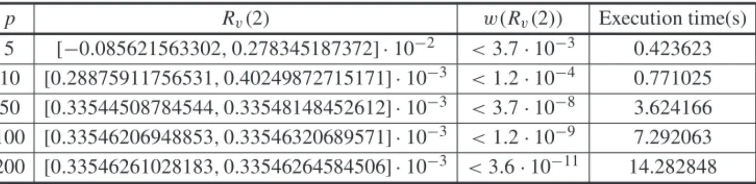
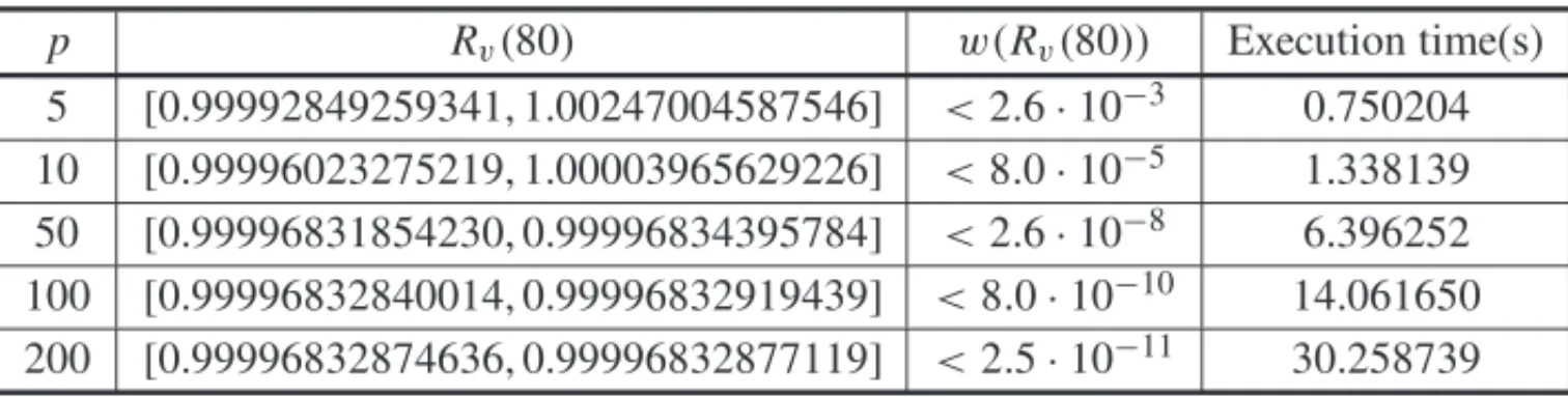
Similarly, we bring another two examples with Exponential and Normal distribution of fail-ures. The Table 3 shows the results in the reliability enclousures computation for an Expo-nential failure distribution system with parameter α = 4. After 2 working-hours, the real-valued reliability function, R(2), and corresponding execution time computation are equal to 3.354626279025164·10−4and 0.050303 seconds. The Table 4 exibiths data from the reliability enclousures computation for Normal failure distribution with parameters µ = 8 and σ = 2. After 80 working-hours, the real-valued reliability function,R(80), and related execution time computation are equal to 0.999968328758167 and 0.087603 seconds.
Table 3: Reliability enclosure, Width of reliability enclosure and execution time, as p are incremented, for Exponential failure distribution system.
p Rv(2) w(Rv(2)) Execution time(s)
5 [−0.085621563302,0.278345187372] ·10−2 <3.7·10−3 0.423623 10 [0.28875911756531,0.40249872715171] ·10−3 <1.2·10−4 0.771025 50 [0.33544508784544,0.33548148452612] ·10−3 <3.7·10−8 3.624166
100 [0.33546206948853,0.33546320689571] ·10−3 <1.2·10−9 7.292063 200 [0.33546261028183,0.33546264584506] ·10−3 <3.6·10−11 14.282848
As we can note in Table 2, Table 3 and Table 4, whenpincreases, the width ofRv(A)decreases.
We can also observe that doublingpthe related interval width is decreased by a factor of 32. All the computed intervals indeed encapsulate the related real-valued reliability function.
Table 4: Reliability enclosure, Width of reliability enclosure and execution time, as pare incremented, for normal failure distribution system.
p Rv(80) w(Rv(80)) Execution time(s)
5 [0.99992849259341, 1.00247004587546] <2.6·10−3 0.750204 10 [0.99996023275219, 1.00003965629226] <8.0·10−5 1.338139 50 [0.99996831854230, 0.99996834395784] <2.6·10−8 6.396252 100 [0.99996832840014, 0.99996832919439] <8.0·10−10 14.061650
200 [0.99996832874636, 0.99996832877119] <2.5·10−11 30.258739
2.2 Mean Time to Failure
Mean Time to Failure (Tmed) of a system is given by the expected value [17] of the random
variableT that specifies its failure process. As pointed out by Kuo and Zuo [13], Tmed is the
lifetime of a system when repairs are not allowed. This metric is
Tmed =
+∞
0
t fT(t)dt. (2.5)
In Equation (2.5), we have that the limits of the integral are 0 e+∞, sinceT assumes only non-negative values.
Proposition 2.2. Let R(t)be the real-valued reliability function of a system. The Mean Time to Failure is
Tmed =
+∞
0
R(t)dt. (2.6)
Proof. On Ebeling [5].
Proposition 2.3.Let Tmed be the real number evaluated by Equation 2.6. If R(t)is a reliability
function, so Tmed <+∞.
Proof. The Equation (2.6) can be represented by the following infinitesimal sum:
Tmed = lim
n→+∞
n
i=1
R(ξi)w([xi−1,xi]),
whereξ1∈ [x0,x1], ξ2∈ [x1,x2], . . . , ξn∈ [xn−1,xn]. The intervals[xi−1,xi],i=1,2, . . . ,n,
are identical partitions of the interval limn→+∞[0,n], considering thatx0=0 andxn =n. We
note that the widthw([xi−1,xi])is identical for all the partitions.
We know thatR(+∞)=0, so, according to [25], we have that the infinitesimal sum is
Based on Equation 2.6, this paper defines the interval function which yields an interval enclosure forTmed.
Definition 2.2. Let T be a random variable that represents the time to failure of a system and
Rv(t)be the reliability enclosure of a specified real-valued reliability function R. Consider the
real number tM AX and a positive integer n, where n → ∞. Suppose the interval[0,tM AX]and
its partitions[x0,x1],[x1,x2], . . . ,[xn−1,xn], where x0=0and xn=tM AX. Also consider that
all partitions have the same widthw= tM AX
n . So, the interval function that encloses the Mean
Time To Failure, considering T , is defined as
Tmedv =n→+∞lim [Rv(tm1)+Rv(tm2)+ · · · +Rv(tmn)]w. (2.7) The valuestm1,tm2, . . . ,tmn are, respectively, the midpoints of the partitions[x0,x1],[x1,x2], . . . ,[xn−1,xn]. For the implementation of the interval function for the mean time to failure,
we use the parameters tM AX andn. So, we must choose the value oftM AX in such way that
R(tM AX) ≈ 0. The value ofn represents the number of partitions of the interval [0,tM AX],
defining the precision in which the interval enclosure is obtained.
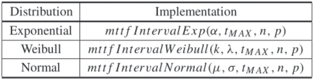
The Table 5 shows the signatures of interval enclosures for mean time to failure for Exponential, Weibull and Normal distributions.
Table 5: Signatures of interval function for mean time to failure.
Distribution Implementation
Exponential mt t f I nt erval E x p(α,tM AX,n,p)
Weibull mt t f I nt ervalW eibull(k, λ,tM AX,n,p)
Normal mt t f I nt erval N ormal(µ, σ,tM AX,n,p)
In the Appendix A, we can observe more details about the implementations of the interval enclo-sures for the mean time to failure for Exponential, Weibull and Normal distributions.
To illustrate the use of Tmedv in bounding the related real-valued metric, assume that T is a
Normal random variable with parametersµ=8 andσ =2. In this case, supposetM AX =16,
which implies that R(16)=6.6613·10−16orR(16)≈0,n =50 and p =5. The real value of mean time to failure for the considered system and the related execution time computation are Tmed = µ = 8 and 2.634465 seconds (this execution cost and all real value of mean time to
failure measures were based on Equation 2.6).
The interval enclosure forTmedis given by
Tmedv = mt t f I nt erval N ormal(8,2,16,50,5)
= [7.98389618066430,8.01618738659977].
In fact, we have thatTmed ∈Tmedv. However, it can be seen that when the conditionR(tM AX)≈
different values oftM AX. It is observed that whentM AX ≤ 12 the intervals do not encapsulate
the real value for the mean time to failure (µ=8).
Table 6: Interval enclosures for mean time to failure, consideringtM AX variation.
tM AX Tmedv R(tM AX)
16 [7.98388828158800, 8.01618934801887] 6.6613·10−16 14 [7.99026276808957, 8.00936514850080] 9.8659·10−10 12 [7.98065312859909, 7.98618574479369] 3.1671·10−5 10 [7.83278842107344, 7.83448378185583] 0.0227
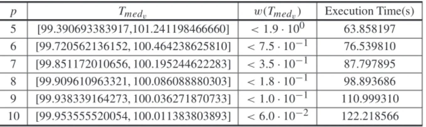
Once the computation ofTmedv involvesn evaluations of Rv, the parameter p is also used to
enclose the mean time to failure. The Table 7 illustrates the variation of the interval widths and related execution times, sincepincreases, consideringtM AX =20 andn=50.
Table 7: Interval enclosures for mean time to failure, consideringpvariation, for Normal failure distribution system.
p Tmedv w(Tmedv) Execution Time(s)
5 [7.95139633268973, 8.06968007167273] <1.2·10−1 46.126105 6 [7.97723844794519, 8.02123846433367] <4.5·10−2 53.791730 7 [7.98380610504386, 8.01751702986318] <3.4·10−2 62.819581 8 [7.99300780057101, 8.00823643857211] <1.6·10−2 70.775011 9 [7.99595743932975, 8.00531274894078] <9.4·10−3 80.984591 10 [7.99776142904487, 8.00352002468972] <5.8·10−3 89.759203
We also bring two examples with Exponential and Weibull distribution of failures. The Table 8 exibiths the results in the mean time to failure enclousure computation for Exponential failure distribution with parameterα=0.01. The real-valued mean time to failure and related execution time are equal toTmed = 100 and 5.925969 seconds. The Table 9 shows data from mean time
to failure enclousure computation for Weibull distribution of failures with parametersk = 3,
λ = 50. The real-valued mean time to failure and corresponding execution time are equals to Tmed =44.642793484075547 and 8.679764 seconds.
Table 8: Interval enclosures for mean time to failure, sincepincreases, consid-eringtM AX =1000 andn=150, for Exponential failure distribution system.
p Tmedv w(Tmedv) Execution Time(s)
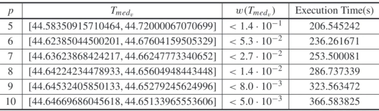
Table 9: Interval enclosures for mean time to failure, since p increases, considering tM AX =120 andn=150, for Weibull failure distribution system.
p Tmedv w(Tmedv) Execution Time(s)
5 [44.58350915710464, 44.72000067070699] <1.4·10−1 206.545242 6 [44.62385044500201, 44.67604159505329] <5.3·10−2 236.261671 7 [44.63623868424217, 44.66247773340652] <2.7·10−2 253.500081 8 [44.64224234478933, 44.65604948443448] <1.4·10−2 286.737339
9 [44.64532405850133, 44.65279245624996] <8.0·10−3 323.563472 10 [44.64669686045618, 44.65133965553606] <5.0·10−3 366.583825
As it is shown in Tables 7, 8 and 9, the interval enclosures for mean time to failure bound corrresponding real values mean time to failure. It also could be observed that the use of interval approach implies a high computation cost, sincenevaluations ofRvmust be done to achieve the
interval proposed. The results brought in Tables 8 and 9, for example, thenvalue employed was 150 to guarantee precision in the interval enclosures.
2.3 Hazard rate function
Hazard rate function,λ(t), is a function that determines an instantaneous failure rate of a system in a specified instantt. The definition ofλ(t)[5] is based on the conditional probability:
P(t ≤T ≤t+ △t|T ≥t)= R(t)−R(t + △t)
R(t) , (2.8)
whereR(t) >0.
Equation 2.8 defines the chance of a system performs its intended function satisfactorily for a specified period of time△t, since do not occur faults in the interval[0,t]. So, the conditional probability presented in (2.8) divided by the time unit (△t) is
R(t)−R(t+ △t)
R(t)△t . (2.9)
Equation 2.9 determines the failure rate per time unit of a system. Thus, the instantaneous failure rate is given by the conditional probability of fault occurences per time unit, when △t → 0. Then,
λ(t) = lim △t→0
−[R(t+ △t)−R(t)]
△t ·
1 R(t)
= −d R(t)
dt ·
1 R(t)=
fT(t)
R(t). (2.10)
Definition 2.3. Let T be a random variable that represents the time to failure of a system and
Rv(t)be the reliability enclosure for its real-valued reliability function R. The interval enclosure
for the real-valued hazard rate function in an instant of time t is given by:
λv(t)=
[∇fT(t),△fT(t)]
Rv(t)
,
where0∈/ Rv(t).
Proposition 2.4.Letλ(t)= fT(t)
R(t). So,λ(t)∈λv(t).
Proof. We know that fT(t)∈ [∇fT(t),△fT(t)]andR(t)∈ Rv(t). Thus,
fT(t)
R(t) ∈
[∇fT(t),△fT(t)]
Rv(t)
⇒λ(t)∈λv(t),
when 0∈/ Rv(t).
The Table 10 illustrates the signatures of interval functions that encapsulate the real-valued haz-ard rate function for Exponential, Weibull and Normal distributions.
Table 10: Signatures of interval function for hazard rate function.
Distribution Implementation
Exponential f ailure Rat eI nt erval E x p(t,p, α)
Weibull f ailure Rat eI nt ervalW eibull(t,p,k, λ)
Normal f ailureRat eI nt erval N or mal(t,p, µ, σ )
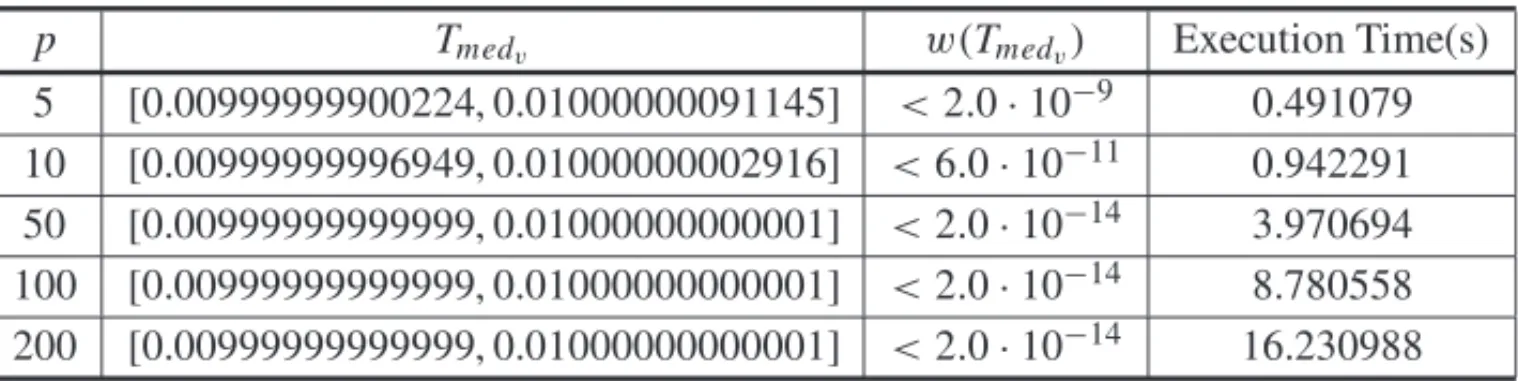
For instance, supposeTis an Exponential random variable with parameterα=0.01. In this case, considering the instantt =100, the real-valued hazard rate function and related execution time are equal toλ(100)=α=0.01 and 0.054298 seconds. The Table 11 illustrates the variation of the hazard rate interval widths and related execution times, sincepincreases.
Table 11: Interval enclosures for hazard rate, considering p variation, for Exponential failure distribution system.
p Tmedv w(Tmedv) Execution Time(s)
5 [0.00999999900224, 0.01000000091145] <2.0·10−9 0.491079 10 [0.00999999996949, 0.01000000002916] <6.0·10−11 0.942291
50 [0.00999999999999, 0.01000000000001] <2.0·10−14 3.970694 100 [0.00999999999999, 0.01000000000001] <2.0·10−14 8.780558 200 [0.00999999999999, 0.01000000000001] <2.0·10−14 16.230988
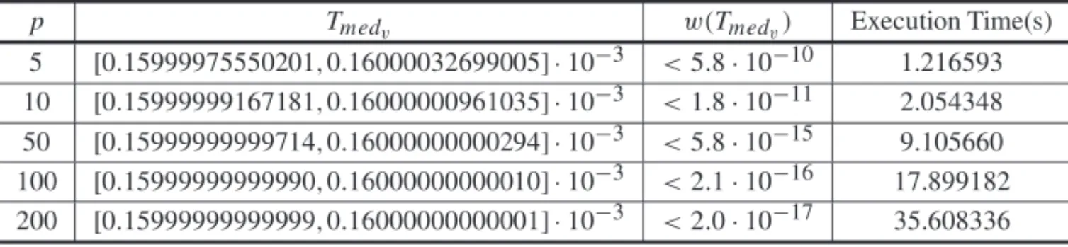
hazard rate function,λ(10), and the related execution time are equal to 1.524830884806074 and 0.095419 seconds. The Table 13 exibiths data from the hazard rate enclousures computation for Weibull failure distribution with parametersk =2 andλ =10000. After 8000 working-hours, the real-valued reliability function,λ(8000), and corresponding execution time computation are equal to 1.6·10−4and 0.101747 seconds.
Table 12: Interval enclosures for hazard rate function, consideringpvariation, for Normal failure distribution system.
p Tmedv w(Tmedv) Execution Time(s)
5 [1.51863640703179, 1.53229224115192] <1.4·10−2 1.008209
10 [1.52460379156082, 1.52507613749420] <4.8·10−4 2.071646 50 [1.52483080854381, 1.52483096220953] <1.6·10−7 11.009327 100 [1.52483088240966, 1.52483088722032] <4.9·10−9 22.419977 200 [1.52483088473101, 1.52483088488142] <1.6·10−10 52.203656
Table 13: Interval enclosures for hazard rate function, consideringpvariation, for Weibull failure distribution system.
p Tmedv w(Tmedv) Execution Time(s)
5 [0.15999975550201,0.16000032699005] ·10−3 <5.8·10−10 1.216593 10 [0.15999999167181,0.16000000961035] ·10−3 <1.8·10−11 2.054348 50 [0.15999999999714,0.16000000000294] ·10−3 <5.8·10−15 9.105660 100 [0.15999999999990,0.16000000000010] ·10−3 <2.1·10−16 17.899182 200 [0.15999999999999,0.16000000000001] ·10−3 <2.0·10−17 35.608336
As the computation process of hazard rate function is similar to reliability function, the execution time of interval enclosure for hazard rate function has the same order of magnitude as the one of reliability enclosure. This could be noted comparing the execution time in examples brought by Section 2.1 and Section 2.3. In Table 11, we can observe that, for p>50, the interval width achieved the least amplitude possible, which shows us that the computation cost of increasing p value does not result in a higher precision.
3 VALIDATION OF INTERVALS FOR COMPLEX SYSTEMS MODELED
IN SHARPE
that is assigned to two different values. Letxibe the state of the i-esimo component of a specified
system. Then,
xi =
1, if the componenti is available, 0, if the componenti is unavailable.
Consider the complex systemLwithncomponents. So, the vectorx =(x1,x2, . . . ,xn)
repre-sents the state of all the components. As well as its components,L also holds one of the two mentioned states. The state ofL, calledφ, is a function of the vectorx. Then, φ = φ (x)= φ (x1,x2, . . . ,xn).
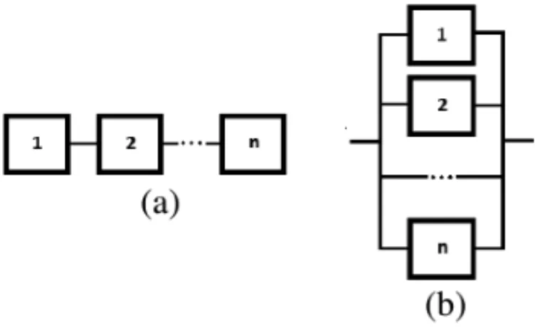
Thus, the functionφ is determined by the components’ configuration of a given system. The following configurations are addressed in this section:seriesandparallel.
Figure 1: (a) Series configuration and (b) Parallel configuration.
The Figure 1(a) indicates that one complex system with components in series [5, 13] exhibits only one critical path. LetLbe the complex system compound byn components in series. The functionφthat defines the state ofLis
φ (x)= n
i=1
xi =min(x1,x2, . . . ,xn). (3.1)
The Equation 3.1 defines that the complex system will fail whether only one of its components fail. So, considering thatL has two components, if only one component failsL also will fail. Thus, assuming that the components’ failure process ofLare independent, the reliability function ofLis given by
R(t)=R1(t)×R2(t)× · · · ×Rn(t)= n
i=1
Ri(t). (3.2)
instant of time. LetL be a system formed byncomponents connected in parallel. The function
φthat defines the state ofLis
φ (x)=1−
n
i=1
(1−xi)=max(x1,x2, . . . ,xn). (3.3)
Therefore, there aren critical paths in the redundant configuration. Thus, the probability thatL does not fail in the period of time[0,t]is given by
R(t)=1−
n
i=1
[1−R(i)(t)]. (3.4)
This section is devoted to validate the proposed reliability enclosures for complex systems. In this way, the SHARPE software [9, 23] was employed in such manner that the real values of reliability function were generated and compared with corresponding interval enclosures. This analysis was accomplished using four case of studies, in which complex systems were modeled in SHARPE. The integration method used in SHARPE was Simpson’s rule [24].
The Matlab software enables two formats to display the computed intervals. The first one is
format shortwhich results fixed-decimal format with 4 decimal digits after decimal point num-bers [15]. The last option,format long, yields fixed-decimal format with 15 decimal digits after the decimal point numbers. The SHARPE software only exhibits 8 significants decimals digits. Therefore, to confirm whether the obtained intervals bound the values computed by SHARPE, we use interval computation with format short configuration. In order to perform the validation of intervals with format long configuration, we use values computed by the previously specified computational platform, which results binary64 numbers displayed, in this paper, with 16 deci-mal digits after the decideci-mal point. In all cases, we use p=200 for all the interval calculations, since, as we will observe, the width of the obtained intervals achieved a reasonable precision.
The computation of the real-valued reliability function was based on systems that have com-ponents with series and parallel configurations simultaneously. According to [5], the reliability function computation of these systems involve their decomposition into subsystems. Thus, the reliability function’s evaluation of each subsystems are done and, then, the obtained values are combined in such way that the reliability function of all the system is calculated. Due to this computation process, the reliability metrics calculated related to complex systems is prone to errors caused by the propagation of round-off and truncation errors.
3.1 Case 1
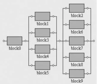
LetW be the system outlined in Figure 2 compound by three subsystems:W1(formed uniquely
by the component block0),W2(formed by the components block1, block3, block4 and block5
connected in parallel) andW3(formed by the components block2, block6, block7, block8 and
block9 also connected in parallel). Consider that the components ofW1has Exponential
Exponential distribution with parameterα1=2·10−11. The real-valued reliability function of W, considering observation timet =20, was evaluated by the SHARPE software and the pre-viously specified computational platform and compared with corresponding interval enclosures (Table 14).
Figure 2: Representation of the systemW, modeled by the SHARPE software.
Table 14: Comparison between the real-valued reliability function of the systemW evaluated by SHARPE,R(20), and the specified computational platform, R(20), and the reliability enclosure, considering short and long configurations.
R(20) 1.00000000
Rv(20)(format single) [0.9999, 1.0000]
R(20) 0.999999999900000
Rv(20)(format long) [0.99999999989999, 0.99999999990001]
We can observe that the interval enclosure with format single configuration contains the value ofR(20). We also note that the computed interval with double precision encapsulates the real value obtained by the specified computational platform. In the case above, we observe that the real-valued reliability function calculated by SHARPE is rounded to 1. So, if we do not use the interval enclosure, the computed value by SHARPE is rounded to the value 1. This might forbidden that comparisons among two systems with different reliability function values close to the real number 1 could be done, since the computed values are rounded to the same punctual value.
3.2 Case 2
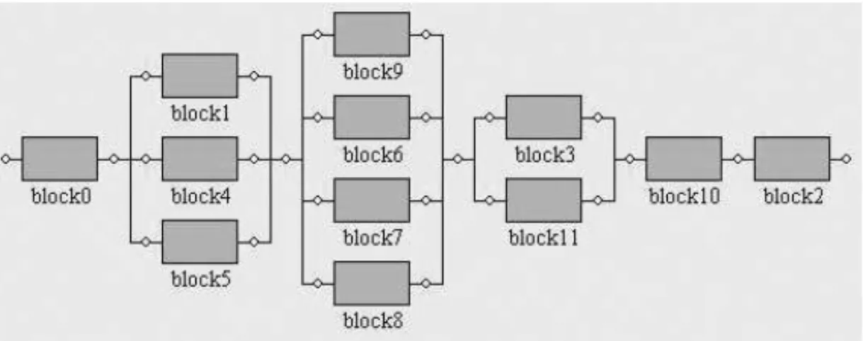
LetM be the system outlined in Figure 3 compound by five subsystems: M1(formed uniquely
by the component block0),M2(formed by the components block1, block4 and block5 connected
in parallel),M3(formed by the components block9, block6, block7 and block8 also connected
(formed by the components block10 and block12 connected in series). Consider that the com-ponents of M1and M5 have Exponential distribution of failures with parameterα0 = 1.2, the
components of M2 have Exponential distribution with parameterα1 = 0.05, the components
ofM3have Exponential distribution with parameterα3=0.08 and the components ofM4have
Exponential distribution of failures with parameterα4=0.5. The real-valued reliability function ofM, considering observation timet =20, was evaluated by the SHARPE software and the pre-viously specified computational platform and compared with corresponding interval enclosures (Table 15).
Figure 3: Representation of the systemM, modeled by the SHARPE software.
Table 15: Comparison between the real-valued reliability function of the sys-tem Mevaluated by SHARPE,R(20), and the specified computational platform, R(20), and the reliability enclosure, considering short and long configurations.
R(20) 0.00000000
Rv(20)(format single) [−0.3364,0.3615] ·10−29
R(20) 2.169808968150444·10−36
Rv(20)(format long) [−0.33637728687207,0.36140951783338] ·10−29
In this study of case (Case 2), we also observe that the computed intervals with single and long configuration enclose the real values obtained by the SHARPE software and the specified compu-tational platform, respectively. In this case, for instance, if we use the reliability value computed by the SHARPE, any multiplication using this numeric value will also result in zero. On other hand, the use of the calculated intervals avoids this type of numeric problem.
3.3 Case 3
LetGbe the system outlined in Figure 4 compound by three subsystems:G1(formed uniquely
by the component block0), G2 (formed by the components block3 and block5 connected in
parallel) andG3(formed by the parallel composition of the subsystems block1 and block6 in
k0 =5, the components of G3have Weibull distribution with parametersλ1 =1 andk1 = 3.
The real-valued reliability function ofG, considering observation timet =1, was evaluated by the SHARPE software and the previously specified computational platform and compared with corresponding interval enclosures (Table 16).
Figure 4: Representation of the systemG, modeled by the SHARPE software.
Table 16: Comparison between the real-valued reliability function of the sys-temGevaluated by SHARPE,R(1), and the specified computational platform, R(1), and the reliability enclosure, considering short and long configurations.
R(1) 0.0780906406
Rv(1)(format single) [0.0780, 0.0781]
R(1) 0.078090640623532
Rv(1)(format long) [0.07809064062237, 0.07809064062470]
As we could observe in Cases 1 and 2, in the Case of study 3 (formed by components with Weibull distribution of failures), we also validate that the computed intervals for Weibull distri-bution enclose the real values obtained by the SHARPE software and the specified computational platform.
3.4 Case 4
LetV be the system outlined in Figure 5 compound by three subsystems:V1(formed uniquely by
the component block0),V2(formed by the components block3 and block5 connected in parallel)
andV3(formed by the components block6, block1, block2, block4, block7 in parallel). Consider
that the component of V1 has Normal distribution of failures with parameters µ0 = 10 and σ0=2, the components ofV2have Normal distribution of failures with parametersµ1=8 and σ1 =2, the components ofV3have Normal distribution with parametersµ2 =12 andσ2=3.
The real-valued reliability function ofV, considering observation timet = 20, was evaluated by the previously specified computational platform and compared with corresponding interval enclosure (Table 17).
computa-Figure 5: Representation of the systemV, modeled by the SHARPE software.
Table 17: Comparison between the real-valued reliability function of the systemV evaluated by the specified computational platform,R(20), and the reliability enclosure, considering long configuration.
R(20) 6.958564143474359·10−13
Rv(20)(format long) [0.69546030782011,0.69625251864393] ·10−12
tional platform and the reliability enclosure with long configuration. As could be observed in the other cases, the interval enclosure obtained for the complex system bounds the related punctual value.
4 CONCLUSIONS
This paper presented a wide set of interval enclosures definitions for reliability metrics, that controls round-off and truncation errors produced by the computation of the corresponding real values. The intervals are obtained using high accuracy in the floating-point system employed.
In order to summary this article, the Tables 18 and 19 outline the main original contributions of this paper. Table 18 shows interval enclosures definitions for reliability metrics. Table 19 presents implementations’ signatures for interval enclosures, considering Exponential, Weibull and Normal distributions.
In Table 18, the interval proposed for reliability function is defined in [16]. The interval defini-tions proposed for mean time to failure and hazard rare function are original contribudefini-tions of this work.
Table 18: Summary of interval enclosures definitions for reliability metrics.
Reliability metric Interval definition proposed
Reliability function Rv(t)= [1,1] −Pv([0,t])
Mean time to failure Tmedv = lim
k→+∞
k
n=1
Rv(tmn)w
Hazard rate function λv(t)= [∇fT(Rt),△fT(t)]
v(t)
Table 19: Summary of implementations’ signatures for interval enclosures, considering Exponential, Weibull and Normal distributions.
Failure distribution Reliability metric IntLab implementation Reliability function con f ex p(t,p, α)
Exponential Mean time to failure mt t f I nt erval E x p(α,max,n,p)
Hazard rate function f ailure Rat eI nt erval E x p(t,p, α)
Reliability function con fweibull(t,p,k, λ)
Weibull Mean time to failure mt t f I nt ervalW eibull(k, λ,max,n,p)
Hazard rate function f ailure Rat eI nt ervalW eibull(t,p,k, λ)
Reliability function con f normal(t,p, µ, σ )
Normal Mean time to failure mt t f I nt erval N ormal(µ, σ,max,n,p)
Hazard rate function f ailure Rat eI nt erval N or mal(t,p, µ, σ )
In this context, the use of interval approach rather than employing punctual values brings an overhead computation cost that must be taken into account. For example, as shown in this work, reliability enclosure computation can spend 10 times more than the real-valued function. Finally, in the four study of cases presented, this paper succesfully validates the reliability enclosure proposed with related real-valued reliability function of complex systems computed by SHARPE software and specified computational platform, considering Exponential, Weibull and Normal failure distributions.
RESUMO. A computac¸˜ao de m´etricas de confiabilidade (func¸˜ao de confiabilidade, tempo m´edio para falhas e taxa de falhas) envolve n´umero reais. Portanto, problemas num´ericos s˜ao
gerados devido `a limitac¸ ˜ao de representar e operar n´umeros reais em computadores. Esse artigo foca no c´alculo de intervalos que limitam erros numericos introduzidos durante o processo de computac¸˜ao de m´etricas de confiabilidade em m´aquinas digitais, considerando
as distribuic¸ ˜oes de falhas Exponencial, Weibull e Normal. Func¸˜oes intervalares foram pro-postas, baseadas na matem´atica intervalar e aritm´etica de exatid˜ao m´axima, para contro-lar erros num´ericos introduzidos pelo c´alculo de valores de m´etricas de confiabilidade para
produzem intervalos encapsuladores para valores reais de m´etricas de confiabilidade e o soft-ware SHARPE foi usado para a validac¸˜ao dos resultados. A an´alise dos resultados num´ericos
obtidos com as func¸˜oes propostas mostraram que os intervalos realmente encapsulam os n´umeros reais calculados pelo software SHARPE, indicando que essas func¸ ˜oes, de fato, s˜ao
uma alternativa para auto-validac¸˜ao desses valores de confiabilidade de sistemas complexos.
Palavras-chave: confiabilidade, matem´atica intervalar, aritm´etica de exatid˜ao m´axima, intervalos encapsuladores.
REFERENCES
[1] M.A. Campos. Interval probability: applications to discrete random variables.TEMA – Trends in Applied and Computational Mathematics,1(2) (2000), 333–343.
[2] M.A. Campos & M.G. Santos. Interval Probabilities and Enclosures.Computational & Applied Math-ematics,32(1) (2013), 413–423.
[3] O. Caprani, K. Madsen & H.B. Nielsen. “Introduction to Interval Analysis”. Technical University of Denmark, Copenhagen (2002).
[4] F.P.A. Coolen & M.J. Newby. “Bayesian Reliability Analysis with Imprecise Prior Probabilities”. Eindhoven University of Technology, Eindhoven (1992).
[5] C.E. Ebeling. “An Introduction to Reliability and Maintainability Engineering”. Waveland Press, Illi-nois (1997).
[6] B.V. Goldberg. What every computer scientist should know about floating-point arithmetic.ACM Computing Surveys,23(1) (1991), 153–230.
[7] P.S. Grigoletti, G.P. Dimuro & L.V. Barboza. M´odulo python para matem´atica intervalar.TEMA – Trends in Applied and Computational Mathematics,8(1) (2007), 73–82.
[8] N.J. Higham. Accuracy and stability of numerical algorithms, 2nd edn. SIAM Publications, Philadel-phia (2002).
[9] C. Hirel, X. Sahner, X. Zang & K. Trivedi. “Reliability and Performability Modeling using SHARPE 2000” (2011). (avaliable in:<http://people.ee.duke.edu/∼kst/>.)
[10] IEEE Standard 754-2008: IEEE Standard for Floating-Point Arithmetic. IEEE Computer Society, New York (2008).
[11] R. Klatte, U. Kulisch, C. Lawo, M. Rauch & A. Wietho. “C-XSC - A C++ class library for extended scientific computing”. Springer, Heidelberg (1993).
[12] U.W. Kulisch & W.L. Miranker. “Computer Arithmetic in Theory and Practice”, Academic Press, New York (1981).
[13] W. Kuo & M.J. Zuo. “Optimal Reliability Modeling: Principles and Applications”. John Wiley & Sons Inc, New Jersey (2003).
[15] The MathWorks Inc, “MATLAB 7.5” (2007). (available in: http://www.mathworks.com/ products/matlab/.)
[16] A.F. Mendonc¸a & M.A. Campos. Confiabilidade Autovalid´avel de Sistemas com Processo Exponen-cial de Falhas.TEMA – Trends in Applied and Computational Mathematics,14(3) (2013), 383–398.
[17] P.L. Meyer. “ Probabilidade Aplicac¸˜oes `a Estat´ıstica”. Livros T´ecnicos e Cient´ıficos, Rio de Janeiro (1983).
[18] R.E. Moore, W. Strother & C.T. Yang. “Interval Integrals”. Technical Report Space Div. Report LMSD703073, Lockheed Missiles and Space Co., (1960).
[19] R.E. Moore. “Interval Analysis”. Englewood Cliffs, New Jersey (1966).
[20] R.E. Moore. “Methods and Applications of Interval Analysis”. Society for Industrial and Applied Mathematics Philadelphia, Philadelphia, (1979).
[21] R.E. Moore, R. B. Kearfott & M.J. Cloud. “Introduction to Interval Analysis”. Society for Industrial and Applied Mathematics Philadelphia, Philadelphia, (2009).
[22] S.M. Rump: INTLAB – INTerval LABoratory. In Tibor Csendes, editor, Developments in Reliable Computing, pages 77-104. Kluwer Academic Publishers, Dordrecht (1999).
[23] R. Sahner, K.S. Trivedi & A. Puliafito. “Performance and Reliability of Computer Systems: An Example-Based Approach Using the SHARPE Software Package”. Kluwer Academic Publishers, Boston (1996).
[24] R. Sahner & K. Trivedi. Reliability Modeling Using SHARPE.Reliability, IEEE Transactions, 36(2) (1987), 186–193.
[25] M. Spivak. “Calculus”. Publish or Perish, Houston (1994).
[26] T. Sunaga. Theory of An Interval Algebra and its Application to Numerical Analysis.RAAG Memoirs, 2(1958), 29–46.
[27] L.V. Utkin. Imprecise reliability of cold standby systems.International Journal of Quality & Relia-bility Management,20(2003), 722–739.
[28] L.V. Utkin. Interval reliability of typical systems with partially known probabilities.European Journal of Operational Research,153(3) (2004), 790–802.
[29] Y. Wang. Imprecise probabilities based on generalized intervals for system reliability assessment.
International Journal of Reliability & Safety,1(2009), 1–23.
[30] J. Yang & H. Sun. Discrete method for structural interval reliability analysis.Chinese Control and Decision Conference,1(2008), 2441–2446.
A IMPLEMENTATIONS OF INTERVAL ENCLOSURES FOR EXPONENTIAL,
WEIBULL AND NORMAL DISTRIBUTIONS
Figure 10: Interval enclosure for reliability function considering component with Exponential failures distribution.
Figure 12: Interval enclosure for hazard rate function considering component with Exponential failures distribution.
Figure 14: Interval enclosure for mean time to failure considering component with Weibull fail-ures distribution.
Figure 16: Interval enclosure for reliability function considering component with Normal failures distribution.