The Competitiveness of the China and India in the European Union

(1)

Technical University of Lisbon

School of Economics and Management (ISEG)

Master in International Economics and European Studies Dissertation

The Competitiveness of the China and India

in the European Union

Student:

Ana Luísa Paulino Coutinho

Advisor:

PhD. Professor Maria Paula Fontoura, ISEG , Lisbon

(2)

Abstract

This paper aims to examine the Competitiveness of China and India in the European Union based on the international trade values, during the time period 2001-2009. It firstly reflects about the ambiguous definition of Competitiveness as well as the diversity of methods that exist to measure this concept. Subsequently, the following work seeks to analyse the exports growth of China and India in particular to the European market.

Therefore, some methodologies were used in this paper: the Revealed Comparative Advantage analysis, which seeks to capture the products where China and

India present Comparative advantage at world’s level; the Constant Market Share analysis, which pretends to verify if the Competitiveness explain the export growth to the European market; and the analysis based on the combination of the Trade Complementarity Index with the Geographical Orientation Index, which permits to identity the products where there is room, for China and India, to expand their exports to the European Union, under certain circumstances.

The empirical analysis suggests that China’s and India’s exports are competitive in products identified by the three methodologies, having in many of them capacity to increase their exports to the European market. However, there still persist high levels of trade protection applied by the European Union, which can explain why China’s and India’s exports have not yet take advantage of their full potential.

(3)

Introduction

The International Trade has been one of the most significant economic subjects studied during the recent centuries. The European Union (EU) became the most important international trade association, given the successive enlargements and the large number of trade registered amongst the group.

However, International Trade has suffered several modifications during the last years. One of the biggest changes has resulted from the strong economic growth of China and India. These two countries have achieved great influence in the World, and are becoming the promise of great economic development in future.

Since the economic development is associated with trade, the following work aims to examine if the exports growth of China and India, in terms of trade goods, are associated with the competitiveness gains in particular in the European market. If it is possible for China and India to increase their exports in the European Union. However, it is necessary to point out that the Competitiveness concept is not consensual to all researches and it can be measured by different methodologies, which can create in

several cases contradictory results.

In this paper, the first chapter will explain the Competitiveness concept according to different contexts as well as several techniques that measure the competitiveness of a country. The second chapter will present the empirical analysis, which is subdivided in three sections. The first section will reflect the bilateral trade of China and India, in particular, with the EU, analysing also which products these two countries present an advantage in the European market. The second section will use the methodology of Constant Market Share that pretends to capture if the raise in Chinese or Indian competitiveness explain the increase on their exports to EU. The third section will use another proposed methodology, which seeks to identify if there are some exported products by China and India where there is trade potential and consequently where it is possible to increase their exports to EU.

(5)

1. The Concept of Competitiveness

1.1.The Economic Competitiveness Context

The competitiveness of an economy has been frequently studied over the last years. However, this is one of the most ambiguous concepts that have been conceived. Generically, it is defined by the country capacity to compete on the international market and the expectation is that, the competitiveness advantage requires a “continuing rise in the living standards of the individuals”, as well as the per capita income, i.e., a country is competitive when it produces with lower product prices than the other competitors. This means that the first country is relatively more productive.

While the theory of International Trade usually relates the concept with the Comparative advantage, initially proposed by Ricardo, or with the Competitive advantage using Management theories1, other perspectives relate the concept of Competitiveness with the environment of the countries where firms are originally located.

For instance, for John Cantwell2 competitiveness means “the possession of the capabilities needed for sustained economic growth in an internationally competitive

selection environment, in which environment there are others (countries, clusters, or individual firms, depending upon the level of analysis) that have an equivalent but

differentiated set of capabilities of their own”. This perspective leads to the consideration of a panoply of factors that determine competitiveness.

Along this line, Abel Mateus3 suggests that the analysis of competitiveness can’t involve only one dimension, simply based, for instance on GDP or productivity. Therefore, the author argues that “countries need to build an environment for their performance that not only encourages the existence of an efficient production structure, such as building institutions and pursue policies that encourage the competitiveness of enterprises.”, which means that the competitiveness does not depend on only one factor, since corporate performance is as necessary as the existence of macroeconomic stability and quality of public institutions.

1

See for instances Porter, M. (1990).

2_{See Cantwell, J. (2006), pp. 544.}

(6)

Because competitiveness involves vague definitions and doesn’t have a rigorous economic theory, Siggel4 proposed several concepts for it. One is the distinction between microeconomics and macroeconomics competitiveness, where the first one is applied to producers or industries, while the second one deals with issues related to the global competition of a country, where, according to the author, “a favorable business climate” is necessary. One possible example of macroeconomic competitiveness is the concept of competitiveness presented by Michael Porter5, who determined five important factors on the national level, which support the competitiveness of a country, designated as Porter’s Diamond. These attributes are Factor Conditions, Demand Conditions, Related and Supporting Industries, Firm Strategy and Structure, and Domestic Rivalry. The combination of these factors determines if a firm has condition to be competitive.

At the microeconomic level the foremost theory is, as already mentioned, the comparative advantage, considered the most consistent theory. The theoretical framework of the comparative advantage will be discussed in the next section in this chapter.

Both the macroeconomic and the microeconomic analysis have been using simple and complex indexes to measure the comparative advantage, which will be summarily explained on the third section of this chapter.

The analysis of economic competitiveness can also have a static or a dynamic approach. According to Siggel6, “one of the major limitations of the principle of comparative advantage (...) is its static nature”, as Ricardo’s theory defines the specialization of a country for a specific time-period. In this sense, it is convenient to apply this concept “as a dynamic indicator of competitiveness” since a competitive advantage of a country is verified when there is an increase on its market share or a change on the productive structure that allows a gain relatively to other country or competitor.

Additionally, the concept of competitiveness can be deterministic or stochastic. The measurement that is usually performed by the literature is deterministic, because it uses costs, prices or market shares that were already observed. The stochastic analysis is based on ex-ante concepts, which measures “the readiness for competition or

4

See Siggel, E. (2007), pp. 5-8.

(7)

potential competitiveness”7. The values on stochastic approach are not directly observed, i.e., it needs to be estimated using for example an econometric model that estimates the trade potential as the investigation deterministic, as it uses the exports and imports values for a time-period already observed. On other hand, it can in part be designated as stochastic, as it provides elements that allow to conclude about trade potential between two countries.

1.2.The Comparative Advantage Concept

The Comparative advantage concept, proposed by Ricardo8, is one of the most used models both in the classical and neoclassical theories. However, the concept has been applied in different economic contexts, which modify the rigorous classical definition of Comparative advantage.

According to Ricardo’s theory, a country should specialize in the product which production is relatively more efficient than the one of its partner. The theory assumes that there is only one productive factor, i.e., the labour, and that there are different technologies in each country.

The Classical model can be generalized for more than two products and two countries. Dornbusch, Fischer and Samuelson(1977)9 applied the model to an infinite number of products, where at equilibrium the products produced by countries are defined by the relative productivities and the ratio of relative wages. In sum, the trade reflects the relative productivity differences between countries for several or for all products.

The most cited investigation of the classical model is the MacDougall(1951)10 test which verified whether the USA industries had higher exports capacity than the UK

industries, industries in which the USA were relatively more productive in the labour factor. The results indicate that in 25 products over 20 satisfies the assumption. However, other investigations verified that at world level the relative labour productivity tends to be higher in countries that are abundant in capital. This can

7

See Siggel, E. (2007), pp. 13.

8_{See the original publication Ricardo, David (1817),}_{On the Principles of Political Economy and}

Taxation, London, John Murray.

9

See Dornbush, Fischer and Samuelson (1977), “Comparative Advantage, Payments in a Ricardian

Model with a Continuum of Goods”, The American Economic Review, vol. 6, pp. 823-839.

10_{See MacDougall (1951), “British and American Exports: A Study Suggested by the Theory of}

(8)

suggest that possibly the results are explained by the Heckscher-Ohlin theory11 and not the Ricardo’s Model.

The Ricardo’s model has been considered unrealistic in terms of specialization, since it was built for the labour factor only. The Heckscher-Ohlin’s (HO) model introduces one more productive factor, such as the capital, and it affirms that one country has comparative advantage in the production that requires intensively the factor that is abundant in that country.

The empirical analysis of the last model above is associated to the Leontief Paradox, which assumes that there is one rich country, the USA, which is abundant in capital. Therefore, the country should export the products that are intensive in capital and import the ones that are intensive in labour. The investigation was applied to the economy of the USA and the results suggest that there is no evidence that the exports are exclusively in products intensive in capital. The author concludes that the country imported more products intensive in capital than exported them, which is considered inconsistent with the theory. However, it has been argued that this paradox possibly can’t be applied to the Heckscher-Ohlin theorem, since it doesn’t analyse the intensive use of the factors per product. It should analyse instead the exports and imports based in productive factors, i.e., the Vanek(1968)12 version of the HO model, which is the adequate one for a world with many factors and products.

In fact, Vanek suggests that the Heckscher-Ohlin theorem needs to be defined in terms of factor services that are incorporated in the trade, i.e., on the net exports. According to this version, a country should export the factor services that are relatively abundant and import the factor services that are relatively scarce. The implications of this study were decisive to the Leontief paradox. According to Leamer(1980)13, using this version the Leontief’ results became compatible with the fact that the USA were capital abundant. Therefore, the Paradox existed only because the test was incorrectly formulated.

The empirical analysis based on the model above is complicated to generalize to various countries. For instance, the production costs must be based in equilibrium prices

11_{See the original publication Ohlin (1952),} _{Interregional and international trade}_{, 2}nd_edition,

Cambridge, Harvard University Press.

12

See Vanek(1968), “The Factor Proportions Theory: The N-Factor Case”, Kyklos, vol. 21, pp. 749-756.

13_{See Leamer(1980), “The Leontief Paradox Reconsidered”,}_{Journal of Political Economy}_{, vol. 88, July,}

(9)

and without any type of distortions. Baldwin(1979)14 concluded that the generalization of the above model for two factors, n products and m countries is not possible. In fact, there is not a critical point in the factorial intensity that leads a country to export all products where it presents higher capital-labour ratios than in the products that are imported, for instance he concludes that the theorem needs to be analysed for each two countries, i.e., in terms of bilateral trade.

When the theory is generalized for more than two factors with several products and countries, according to Deardorff(1980)15, it is only guaranteed that there is a correlation between Comparative advantage and trade direction. It can’t be affirmed anything with rigour about a particular firm or industry.

During the 70’s and 80’s, Krugman and other authors16 sought to build international trade models that explain the export advantage based on more realistic assumptions. This line of reserach permits an improvement on the analysis of the firm’s characteristics that participated on the international trade. Based on the monopolistic competition, the researchers have followed two investigation types. On one hand, new aspects as the product differentiation, economies of scale and monopolistic competition were incorporated in the traditional model. According to Helpman(1981)17, this new investigation allows to generalize the Heckscher-Ohlin model, since it explains, based on the factorial allocation, the pattern of specialization as well as the relation with the

intra-industry trade.

On the other hand, some investigations have been done in the oligopoly context, which reveals that identical economies that produce homogeneous products can penetrate on the partner market by discriminating the prices18. This approach also allows to introduce the horizontal and vertical product differentiation analysis19. In this

14

See Baldwin(1979), “Determinants of the Commodity Structure of US Trade”, American Economic Review, vol. 61, May, pp. 126-146.

15_{See Deardorff, A. (1980), “The General Validity of the Law of Comparative Advantage”,}_{Journal of}

International Economics, vol. 9, pp. 197-209.

16

See Krugman (1979), “Increasing Returns, Monopolistic Competition and International Trade”, Journal of International Economics, vol. 9, pp.469-479; Krugman (1980), “Scale Economies, Product

Differentiation and the Pattern of Trade”, American Economic Review, vol.70, nº5, pp.950-959; Lancaster

(1980), “Intra-Industry Trade under Perfect Monopolistic Competition”, Journal of International Economics, vol.10, pp.151-175.

17

See Helpman (1981), “International Trade in the Presence of Product Differentiation, Economies of Scale and Monopolistic Competition”, Journal of International Economics, vol. 11, pp. 305-340.

18_{See Brander (1981), “Intra-Industry Trade in Identical Commodities”,}_{Journal of International}

Economics, vol.11, pp. 1-14; Brander and Krugman (1983), “A Reciprocal Dumping Model of International Trade”, Journal of International Economics, vol. 15, pp. 313-321.

19_{See Eaton and Kierzkowski (1984), “Oligopolistic Competition, Product Variety and International}

(10)

case, the analysis is different from the general theory of the trade pattern, since there are modifications on the initial assumptions. It is possible to still consider the Comparative advantage concept in the context of this new modelling but in fact we have a different concept. So some authors prefer to rename the Comparative advantage concept as Competitive advantage20 to signal that we are considering a new approach.

Finally the Comparative advantage concept has also been enlarged to a new paradigm, which considers localization factors. Krugman(1991,1993)21 affirms that the change on the paradigm is visible when the economic theory recognizes the importance of the geographical location of the production as an explanation to the international trade. This paradigm is not recent, but no doubt the importance of the external economies of scale at regional level to explain the location of economic activity and determine the trade patterns rose during the last decade.

1.3.The Measure of Competitiveness

The methods of analysis of international competitiveness are very diverse and depend on the investigation objectives. But it can be grouped into two areas of analysis, the macroeconomic and the microeconomic areas.

On the Macroeconomic field, simple or complex indexes can be used. There are several simple indexes and they are selected according to the objective that the researcher wishes to analyse. For example, the Labour unit cost, which is the ratio of the total remuneration per worker over the GDP per person employed, at current price. It shows the relation between the remunerations and productivity per worker that permits to analyse if a country is more competitive, which occurs if for the same value of salaries, there is an increase on the GDP per person employed. Another index is the Real Effective Exchange Rate, which is one of the most used indexes. It captures the competitiveness of a country without exclusive dependence on Nominal Exchange Rate or the Inflation level: if there is a real appreciation it signifies that there is a competitiveness lost.

Press, Oxford; Shaked and Sutton (1984) “Natural Oligopolies and International Trade”, in Kierzkowski

(ed.) (1987), Protection and Competition in International Trade, Basil and Blackwell, Oxford.

20

According to Siggel, E. (2007).

21

See Krugman (1991), Geography and Trade, Cambridge, MIT Press; Krugman (1993), “On the

Relationship between Trade Theory and Location Theory”, Review of International Economics, vol.1(2),

(11)

Relatively to the complex indexes, which consider several factors that influence the productivity of an economy, they are defined by institutions such as World Economic Forum (WEF). The WEF global competitiveness index “is based on 12 pillars of competitiveness, providing a comprehensive picture of the competitiveness landscape in countries around the world at all stages of development. The pillars are: institutions, infrastructure, macroeconomic environment, health and primary education, higher education and training, goods market efficiency, labour market efficiency, financial market development, technological readiness, market size, business sophistication and innovation”22. In the end, the index ranks the countries according to their results. Another Index is the Networked Readiness Index that determines the country capacity to use the information and communication technology and compares it with other countries’ capacity. There are other Indexes, such as the Global Competitiveness Index made by the International institute for Management and Development or Trade and Development Index defined by the UNCTAD.

On the Microeconomic field various indexes can also be used, but there are some that are more interesting, such as the Revealed Comparative Advantage(RCA)23, which is based on the Ricardo’s Comparative Advantage. The objective is to determine the country’s competitive sectors by analysing the trade flow to the trade partner24, assuming that these flows reflect the patterns of specialization. Another Microeconomic

index is the Market Share, which affirms that one country is more competitive in one sector if the market share in that sector increases.

The export performance Balassa’s index is the most common index of RCA or more rigorously, as Siggel25 affirms, the Competitive advantage, considering that it does not in fact capture the pure concept of Comparative advantage. The Balassa’s RCA can be measured through two methods, the relative exports index or the export-import ratio, however it is recommended to use the first one, since the imports value contains the trade protection included, which can influence the analysis.

22_{See WEF website available at}_{http://www.weforum.org/issues/global-competitiveness}_{[accessed at}

August 2011].

23

See Balassa (1965), “Trade Liberalization and Revealed Comparative Advantage”, The Manchester

School of Economics and Social Studies, vol.33, nº2, pp. 93-125.

(12)

This index, using the relative exports, has been criticised by several researchers, as mentioned in Fontoura(1997)26, namely Hillman(1980), which affirmed that the index wasn’t appropriate to compare several products for the same country, Yeats(1985), which concluded that the RCA rank per industry for each country was different of the RCA rank for the same industry per country, or Bowen(1983), which concludes that the cardinal value of this index doesn’t permit to conclude about Comparative advantage. However, Vollrath(1991) concludes that, in spite of all criticism, this RCA is the most appropriated index to measure the Comparative advantage. It is worth mentioning that there are other indexes also based on pos-trade values that have been used, which are as well inspired on Balassa’s index.

On the following empirical analysis we will use Competitiveness at the Microeconomic level. Besides the traditional RCA index proposed by Balassa, as mention above, in section 2.3 two other indexes will be used: the Trade Complementarity Index (TCI) and the Geographical Orientation Index (GOI), since combining these two indexes may provide information about the trade potential.

26

See in Fontoura, M. P. (1997): Hillman(1980), “Observations on the Relation between “Revealed Comparative Advantage” and Comparative Advantage as Indicated by Pre-Trade Relative Prices”, Weltwirtschaftliches Archiv, vol.116, pp. 315-321; Yeats (1985), “On the Appropriate Interpretation of the Revealed Comparative Advantage Index: Implications of a Methodology Based on Industry Sector

Analysis”, Weltwirtschaftliches Archiv, vol. 121, pp. 61-73; Bowen (1983), “On the Theoretical

Interpretation of Indices of Trade Intensity and Revealed Comparative Advantage”, Weltwirtschaftliches

Archiv, vol. 119, pp. 464-472; Vollrath (1991), “A Theoretical Evaluation of Alternative Trade Intensity

(13)

2. Empirical Analysis

2.1.Overview of Trade of China and India with European Union

The aim of this chapter is to provide an overview of recent developments in the export trade of China and India in terms of trade goods.

The exports of China and India have increased substantially over the past years. According to WTO27, these two countries, respectively, exported to the World in 2009 about 9.6% and 1.32% of the World trade of merchandise. The large annual percentage of merchandise exports, from 2000 to 2009, is respectively for China and India about 19% and 16%, which reveals that these two economies increased their presence in the international trade during the last years.

In the case of China, the productive structure is characterized by exports specialization almost only in Manufactured products. As per Graph 1, since 2001 until 2009 the share of Agricultural products on the Chinese exports to the world registered a decrease as well as the Fuel and Mining products. In the Indian case, as per Graph 2, the exports specialization presents a significant share of Agricultural products with a slight decrease trend over the period analysed. The Fuel and Mining products present an

increase in the exports share to the world between 2001 and 2009. For the same time period, the Manufactured products represent about 65% of the Indian exports. The

Chinese productive structure, comparatively to India, is more specialized in Manufactured products. Therefore, it presents a lower exports share on the Fuel and Mining products as well as on the Agricultural products.

The China’s exports analysis can be based on the Lorenz Index28 (Graph 3), which verifies if there was a change on the China’s export structure for a specific time period. The results suggest that between 2001 and 2009 there was a significant variation on Chinese structure, being more significant in the time period 2001-2005 than in 2005-2009. For Indian case, the Lorenz Index results (Graph 4) reveal that the changes on the export structure are slightly higher in the time period 2001-2005 than in 2005-2009. The

27

See WTO statistics database available at the website respectively for China and India http://stat.wto.org/CountryProfile/WSDBCountryPFView.aspx?Language=E&Country=CN,IN

[Accessed at May 2011]

28

The Index is given by LI = abs[(Xijg1/XijT1) – (Xijg0/XijT0)], where Xijg1 represents the China or India

export to UE(15) of the product g at the final of the time period; XijT1 represents the total exports at final

of the period; Xijg0 and XijT0 represent, respectively, the product and the total export at the beginning of

(14)

China’ index presents a smaller result than the Indian index for the three time periods, which means that India’ specialization had a higher variation comparatively to China.

The China and India exports can be analysed using the share of each group29 over the total exported particularly to the EU(15)30 in a specific time period. According to Graph 5, the groups 20, Clothing, and 27, Machinery, present in 2001 a significant share, representing respectively about 9% and 37% of the total exported. In 2009 the same groups almost dominated the China’s exports, since they represent proximally 14% and 45% of the total exported. The results suggest that there was a positive exports trend growth on both groups during the time period analysed. It is worth pointing out that the Machinery sector represented the majority of Chinese exports in 2009.

Concerning the Indian case, as per Graph 6, group 20, Clothing sector, is the most significant group in 2001 and 2009, representing respectively 22% and 19% of the total exported. The results suggest that this sector has had a decrease in its importance in India export to the European market. In 2001 the group 23, Precious Metals and Stones, present also a significant share, about 12% of the total exported. In 2009 there were another two significant groups 8, Mineral Fuels, and 28, Automobiles and other transports as well as their accessories, which represent respectively about 15% and 10% of the total exported, with a positive exports trend of growth during the time period analysed.

Regarding the China and India exports to the EU(15) by category of products, the following analysis is based on the variation of the share of each group in the total. For China during the time period 2001-2009, as per the Graph 7, the variation is positive and more significant on the groups 27 and 20, which represent respectively the Machinery and Clothing sectors, and it is negative on groups 9, 15 and 21, which represent respectively the Chemical, Raw skins, Leather or Artificial Fur, and Footwear sectors. On group 27 there is a negative variation between 2005 and 2009, which means that there was a decrease on the exported value of this group or an increase of other group exports that increased the total exported value. On group 20 the positive variation on the time period 2005-2009 is higher than on 2001-2005, which means that on the last few years the exports share to EU(15) increase more than on the first years of the decade. In India’s case, as per Graph 8, groups 8, 24, 27 and 28 present a positive and more significant variation in the period 2001-2009, it means that the exports share

29_{For more information concerning the groups’ classification please see Data Appendix in Annex.}

(15)

increase for Mineral fuels, Iron Steel and Copper products, Machinery or Automobiles sectors; groups 3, 15, 18, 19, 30 and 23 present a negative variation between 2001 and 2009, it means that the exports share decreased for Raw skins, Leather, Cotton, Wool, Rugs and similar sectors.

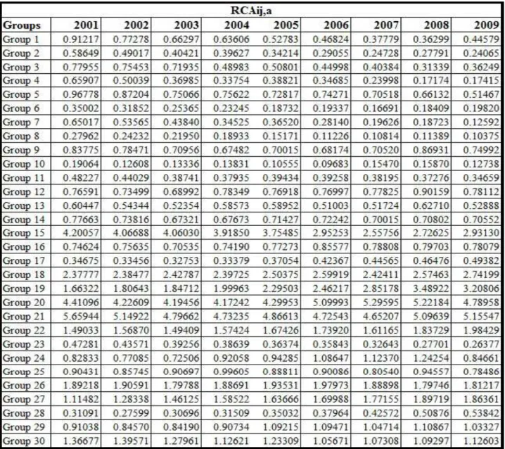
2.1.1. Revealed Comparative Advantage for China and India

The analysis of the competitiveness of trade of China and India with EU(15) can be made based on the Revealed Comparative Advantage index, proposed by

Balassa(1965)31. As mentioned before, it is the traditional way to capture the country’s competitiveness on the trade partner market. The RCA32 index is calculated as follows:

Where i represents the exporter country, China or India, a is a particular product, X represents the exports and M represents the imports (excluding the World imports made in China33). If the RCA is higher than one, it means that the exporter country is competitive in the specific product. If the RCA is lower than one, it means that the

exporter country has a disadvantage in the analysed product.

As per Table 234, China’s total exports are competitive between 2001 and 2009 for groups 15, 18-22, 26, 27 and 30. It means that in products as Raw skins, Leather, Silk, Wool Cotton, Rugs, Clothing, Footwear, products made by Slate, Brick, Porcelain or Machinery and Tools instruments, China is competitive at World’s level. From 2005 until 2009, China displays competitiveness as well on groups 24 and 29, i.e., in products as Iron, Steel and Copper or Electro-medical apparatus and Laboratory equipment and similar. In sum, China presents an advantage essentially in the Traditional Sector, i.e., Footwear, Clothing and Textile products, and on the Machinery and Transport Sectors, which require more technology and qualified workers.

31

See Balassa (1965), “Trade Liberalization and Revealed Comparative Advantage”, The Manchester School of Economics and Social Studies, vol. 33, n.º2, pp. 93-125.

32_{According to the RCA index defined in Castilho (2003), pp. 222. It is an adoption of the RCA}

explained above, which use the Worlds imports instead of the Worlds exports. Therefore, the methodology can be overestimate the competitiveness of both countries, since it is not eliminated the trade protections.

33_{It is removed the intra-trade between the economies and the World, since this trade relation is already}

determinate by the trade preferences.

34

The Empirical analysis used the annual product export at the trade goods during 2001-2009. The methodology was applied for the 30 groups created as well as for the 4-digit level disaggregation. For more information see the Data Appendix in Annex.

(16)

Rodrik(2006)35 analysis affirmed that “Chinese exports often concentrate on the more labour-intensive, less sophisticated end of the product spectrum, at least when we compare them to the exports of significantly richer countries”. The author adds that “Chinese exports of electronics products tend to be low-cost, high volume products with not much technological sophistication (...)”, which explain the Chinese advantage in electronics and machinery production at World’s level.

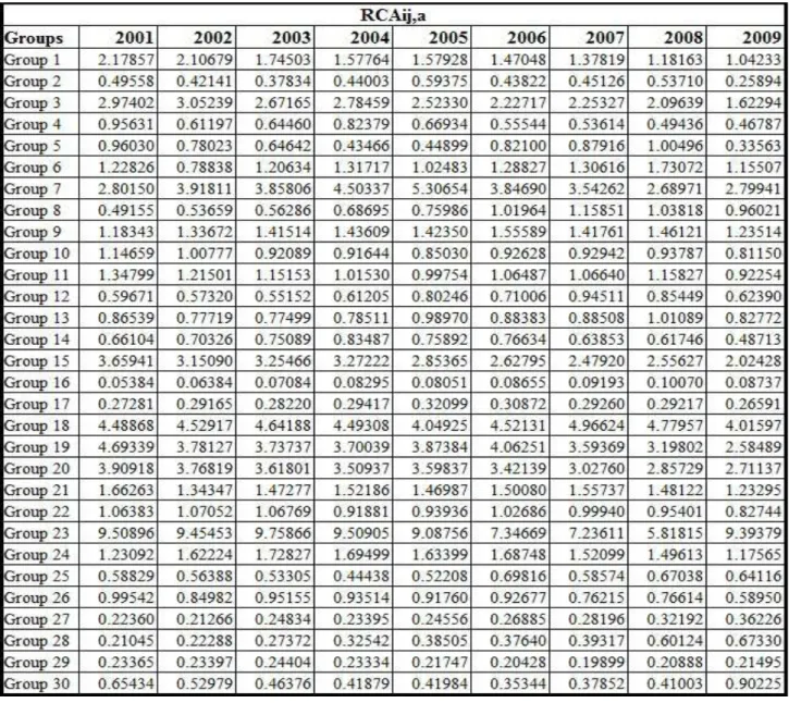
Regarding the Indian case, as per Table 3, there was competitiveness between 2001 and 2009 on groups 1, 3, 7, 9, 15, 18-21, 23-24, i.e., in Agricultural products, as Cereals or Vegetables, in Ores and Metal products, Chemical and Organic compounds, Raw skins, Leather, Silk, Wool and similar products, Clothing and Footwear, Precious metals and Stones, or in Iron, Steel and Copper products. During this time period, India’s exports also present competitiveness in some years on groups 6, 8, 11-12, i.e., in products as Mineral Fuels, Organic Substances or Beauty and Make-up preparations.

Indian total exports present a significant advantage in the Traditional sectors as well as in the Agricultural, Metals and Chemical sectors. It can suggest that most of the products that India presents competitiveness are in the primary and labour intensive sectors.

2.2.Does Competitiveness explain export trade?

The following methodology aims to ascertain whether competitiveness of China and India explain the export growth of these two countries on the European market. For this purpose we perform a Shift-Share analysis.

2.2.1. Methodology

The Shift-Share analysis, or Constant-Market-Shares (CMS) analysis, was first applied in the “pioneering work of Tyszynski (1951)”36. It is a decomposition technique, which describes the increase in the exports of a country into different components. The purpose of breaking down the analysis of exports growth in a country is that it takes into account the specific commodity structure as well as the particular composition of the export markets of the total exported. On one hand, the products

(17)

exported can contain several goods for which the world’s demand is relatively slowly, the case for example of the primary products. This induces that the country's exports may increase slowly and its market share being negatively affected. On other hand, the composition of the export markets of a country can also influence its exports growth. Both factors need to be determined as of the exports growth, since they are not related with a possible increase on the country's competitiveness. With this technique it is possible to measure the competitiveness effect to the growth of trade assuming that for the total export growth rate it is taken into consideration the export growth rate at constant market share.

The following empirical analysis adopts the CMS identity suggested by Jepman, C. (1981)37, which is given by:

Where ∆q=∆[ΣiΣjqij] means the total variation per product of country’s exports to the world between the time period, i.e., the growth of country’s exports; S0=q0/Q0 is the share, per product i, of country’s exports over the total world’s exports at the beginning of the time period; ∆Q=∆[ΣiΣjQij] means the difference on total world’s exports between the time period analysed; Si0=qi0/Qi0 is the share, per product i, of country’s exports to the world over the total world’s exports at the beginning of the time

period; ∆Qi is the difference on world’s total exports per product i between the time period; Sijo=qij0/Qij0 is the share, per product i, of country’s exports to a specific country/market j over the world’s exports to country/market j at the beginning of the period; ∆Qij means the difference on world’s export to a specific country/market j per product i between the time period; ∆Sij means the difference on the share, per product i, of the country’s exports to country/market j over the world’s exports to country/market j; and Qij1 is the value of world’s export to country/market j at the end of the time period.

The Total Effect captures the exports performance of a country during a specific time period, and it is decomposed into the Scale Effect, Product Effect, Market Effect and Competitive Effect.

The Scale Effect represents the change on a country’s exports when its growth is equal to the world export growth in terms of commodity and market. This effect “shows

37_{See Jepma (1981).}

TE SE PE ME CE

(18)

how much the exports would have increased had the percentage change of the total export been the same as that of the total export of the standard”38, where the standard means the group of countries that are the comparative group of exports performance.

The Product Effect allows us to analyse if the exports specialization in a specific product, or in several products, is relevant for the total exports growth in a specific time period. If this effect presents a positive value, it means that the product structure results in a beneficial influence on country’s exports.

The Market Effect reveals if the destination market has an impact in the country’s exports growth. If the export markets have a harmful influence on the country’s exports, then this effect comes negative.

The Competitive Effect is the “residual” term and it “represents both the influence of price and volume competition”39 on the exports growth, i.e., it mirrors the country’s capacity to increase its market share. However, it is very difficult to capture the influence of the price and volume competition on the residual term. One important point to note is that the exports data is generally in USD value, instead of domestic currency. Hence developments in market share are influenced by variations on USD exchange rate. It means that, ceteris paribus, an appreciation of the USD will result in a decline in the market share of the country analysed.

Some critiques have been made to this method, as Baldwin(1958) and

Richardson(1971), whom considered it “an index of number approach in which different weights of aggregation can be chosen in order to obtain consistency in accounting for changes in total exports (or exports shares)”40, i.e., the formula is sensitive to level of disaggregation, range period or geographical groups used on empirical analysis, which can give different results for the same export’s country. For example, the Scale Effect can present different results according to the comparative groups selected. Therefore, it is recommended to define this group as the group that contains the most important competitors of the country analysed.

There is another issue concerning the measure of the Product Effect and the Market Effect, since in the Market Effect we subtracted part41 of the Product Effect and for instance, if it is used a similar term42, the sum of both Effects will not change,

38_{See Jepma (1981).} 39

See Jepma (1981).

40

See Milana, Carlo (1988).

41_{It is used the following term:}

ΣiSi0*∆Qi

42_{Which can be the following term:}

(19)

however the individual results would be different. It reflects the arbitrary that there is on the choice of the terms used in this methodology.

Richardson also mention that “the problem is that over the time period under consideration, both a country’s export structure and world exports are continuously changing. The typical research however, has observations in only the beginning and end of period variables, while he optimally would like to know (...) at every moment during the period”43, i.e., using discrete time.

In the next section we present the empirical results obtained with the methodology presented above calculated for two sub-periods between 2001 and 2009.

2.2.2. EMPIRICAL RESULTS

The following analysis of the China and India export performance uses annual product exports of trade goods during 2001-200944. The methodology was applied for the 30 groups created for this purpose as well as for the 4-digit level disaggregation.

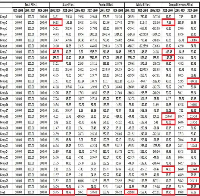
Table 4 reports the results for China’s exports between 2001 and 2009. The Total Effect presents a positive value in all groups, revealing that there was an increase in China’s exports to the EU(15). However, if the results were analysed for the time period 2001-2004 one verifies a negative Total Effect on group 2 and for period 2005-2009 in groups 7 and 8. It can suggest that there was a drop in export to European market in products as Animal products or its derivates in the first sub-period analysed and in products as Ores and Metal products or Mineral Fuels on the second sub-period analysed.

It is worth mentioning that the Total Effect on the time period 2001-2009 is higher on groups 27, Machinery and other equipment, and 20, Clothing, representing

about 46.52% and 15.23% of the Total Effect, respectively. It means that these two groups were the ones that contributed more for the growth of China’s exports in the period analysed.

According to the following Table, the China’s exports growth was essentially explained by the Competitive Effect, since it represents about 95% of the Total Effect in

43

See Richardson, J. D. (1971), “Constant-Market-Shares Analysis of Export Growth”, Journal of

International Economics, vol. 1, pp. 227-239.

(20)

the time period 2001-2009. It means that Chinese growth is basically given by the increase on its capacity to export to EU(15).

The Market Effect represents proximally -110% of the Total Effect in the time period 2001-2009, which means that the EU(15), as a destination market, has a negative influence on the Chinese exports growth. The Product Effect represents about 108% of the Total Effect in the same time period, which means that Chinese specialization is favourable to its exports to the EU(15).

Finally, the Scale Effect, related to the world export growth, represents only about 16% of the Total Effect, being proximally one-third in the period 2001-2004.

Table 5: China’s results of the Constant Market Share analysis per group between the

time period 2001 and 2009, and the sub-periods 2001-2004 and 2005-2009

Source: Own calculations using data available at the Website of International Trade Centre:

(21)

Focussing the Competitive Effect, effect with more significance, it presents between 2001 and 2009 a positive value for all groups, except for groups 2, Animal products or derivate, 7, Ores and metal products, and 8, Mineral Fuels. It means that in these three groups China decreased its capacity to export to the European Market. In the same time period, the groups that present a higher value of Competitive Effect are 18, Silk, Wool, Cotton, Fabrics, Synthetic Fibbers, 19, Rugs, Tulle, Padded, Textile coatings, and 27, Machinery and other equipment. These groups, which present the most significant Competitiveness Effect, together, represent in 2009 about 46% of the total exports to EU(15).

If we consider the sub-period 2005-2009, the Competitive Effect presents a negative value in groups 5, Prepared, Preserved or Extracts of products, and 12, Waxes, Albumin and other organic substances. It presents higher values in groups 16, Wood and its products, 23, Precious Metals and Stones, and 28, Automobiles and other transports as well as their accessories, as did in groups 18, 19 and 27. Together, the most significant groups, represent in 2009 about 50% of the total exports to the EU(15). It means that the majority of the China exports are explained by the raise of its competitiveness.

It is worth pointing out some values on the Scale Effect, since groups 2, 7 and 8 present a higher percentage of Total Effect between 2001 and 2009. It possibly means

that the weak competitiveness into the European Market in the case of these groups can be explained by the equal change in China’s exports as well as in the world’s exports.

Analysing the results at the 4-digit level45, it reveals that the highest percentage of the Total Effect on the period 2001-2009 is in product 8471, Automatic data process machines, optical reader and others, which presents about 13.94% of it. It is interesting to observe that it is mainly explained by the Competitive Effect, representing in this particular product proximally 99% of the Total Effect.

It is worth mentioning, also, the product 8517, Electric apparatus for line telephony including current line system, as it presents a high Total Effect in the period 2005-2009, about 11.41 % and this effect is essentially explained by the Scale Effect and Competitive Effect. Therefore, the growth of China exports in this product is given by an increase on World’s exports, about 10.8% of the Total Effect in this specific product, and by an increase of China competitiveness, of about 89.19%.

(22)

Another relevant results are the product 6110, Jerseys, pullovers, cardigans and others, knitted or crocheted, which represents 3.90% of the Total Effect in the period 2005-2009; or the product 6204, Women's suits, jackets, dresses skirts and shorts, that presents about 2.56% of Total Effect for the same period. Indeed, the rises of the exports of both products are essentially given by an increase on the Competitive Effect, since this effect represents, respectively, about 95.01% and 92.87% of Total Effect of each product.

It is worth pointing out that the products, mentioned at the 4-digit level analysis, represent, together, in 2009, proximally 21.37% of the China’s exports to the EU(15). It means that about one-fourth of the China exports are explained by it competitiveness in this specific market.

Regarding now the results for Indian exports, according to Table 6, the Total Effect was positive for all groups between the time period 2001 and 2009, which reveals that India registered a growth on its exports. However, if the results were analysed for the time period 2005-2009, groups 2, 7, 18 and 19 present a negative Total Effect. It means that there was a decrease in Indian exports during this time period in products as Animal Products or its Derivates, Ores and Metal products, Silk, Wool, Cotton, Fabrics, Synthetic Fibbers, or Rugs, Tulle, Padded and Textile coatings.

It is worth mentioning that the Total Effect of the time period 2001-2009 is

higher on groups 8, Mineral Fuels, 20, Clothing, and 28, Automobiles and other transports as well as their accessories, representing, respectively, about 21%, 18% and 13% of the TE. It means that these three groups were the ones that contributed more for the growth of Indian exports in the period analysed.

According to the following Table, Indian exports growth was mainly explained by the Competitive Effect, since it represents about 69% of Total Effect in the time period 2001-2009. It means that India’s growth is given in part by the increase on its capacity to export to EU(15).

(23)

The Scale Effect represents about 31% of Total Effect, being higher in the period 2005-2009 where it is about 72%. Nevertheless, this effect is less relevant than the Competitive Effect.

Table 7: India’s results of the Constant Market Share analysis per group between the time period 2001 and 2009, and the sub-periods 2001-2004 and 2005-2009

http://www.intracen.org/ [accessed at February 2011]

(24)

its exports to EU(15) is given by products as Animal Products or its Derivates, Paints, Varnishes and other Beauty and Make-up preparations, or Precious Metals and Stones. These groups together represent, in 2009, about 9% of the Indian exports to the EU(15). The results suggest that the competitiveness of Indian exports is in products that present a lower share of the total exports to the European market.

Analysing the results at the 4-digit level, it reveals that the product 2710, Petroleum oils, not crude, is the one that presents the highest value in the period 2001-2009, about 21.05% of Total Effect. This is essentially explained by the Competitive Effect, since it presents about 100% of the Total Effect of this specific product. Other relevant results are the products 8703, Cars, including station wagon, 8803, Aircraft parts, 8901, Cruise ship, cargo ship, barges, since they present respectively about 7.49%, 1.65% and 1.61% of Total Effect in the period 2001-2009 and in the sub-period 2005-2009, receptively, 12.01%, 3.35% and 2.93%. The increase in these products is mainly explained by the Competitive Effect, since it represents between 2001 and 2009, respectively, about 98.61%, 86.45% and 99.93% of Total Effect of each product.

It is worth pointing out that the products, mentioned at the 4-digit level analysis, represent, together, in 2009, about 22.69% of the India’s exports to the EU(15). It means that proximally one-fourth of the India exports are explained by it competitiveness in this specific market.

In sum, according to the analysis above, both exports trade for each country present several products or sectors where the growth is essentially explained by the rise on its competitiveness. On one hand, China exports products, such as Silk, Wool, Cotton or similar products, Clothing or Machinery, are explained by its competitive effect, i.e., its capacity to increase its exports in the European market. It suggests that China’s competitiveness is in products that it presents a higher significance in the total exported, i.e., in Traditional Sector as well as in more sophisticated sector, such as the Machinery.

(25)

2.3. Complementarity and Geographical bias: Is there potential to increase trade?

China and India exports have registered a strong growth during the recent years, as did their presence on the international market. However, is it still possible to raise their exports for the EU markets? In which products? The following methodology, adopted from Castilho and Flôres46, provides some information on this respect.

2.3.1. Methodology

Castilho and Flôres(2005) combine an analysis based on the revealed comparative advantage indexes, with a “geographic orientation” dimension introduced. The methodology is based in two indexes, the Trade Complementarity Index (TCI) and the Geographical Orientation Index (GOI).

The TCI is defined as the product of the exports RCA with the imports Comparative Disadvantage Index (CDM), which analyses the correspondence between the supply from the exporter country and the demand from the trade partner. The RCA is given by the country’ share of exports of a product in total over the world’ share of imports of the same product in total (excluding the world’s imports from the exporter country). The CDM is given by the partner’s share of imports of the same product in total over the the world’ share of imports of the same product in total (excluding from the world imports those that are made to the trade partner). The index is calculated as follows:

Where, i represents the export country, j the trade partner, w the world, a the specific product, X the exports value and M the imports value. When TCI value is higher than one it means that there is trade complementarity, since the exporter country presents a superior competitiveness and satisfies the demand of the trade partner. Therefore, it is expected that with the trade liberalization more trade will occur between

both countries.

The GOI is defined as the ratio, for a specific product, between the country’ share of exports to the trade partner in the total and the partner’ share of imports in the world’s imports (excluding the world’s imports those that are from the exporter

46_{See Castilho and Flôres (2005)}

(26)

country). It aims to verify the existence of geographical bias, i.e., if the exports capacity for the trade partner are undervalued and then the exporter country has possibility to export more to the importer country. The index is calculated as follows:

Where the i represent the export country, j the trade partner, w the world, a the specific product, X the exports value and M the imports value. If the result of GOI is higher than one it means that there is a "positive" geographical bias, since for a specific product the exports made by the country i in the total exported are superior to the imports made by the partner in the world. If it is negative, it means that there is room to expand export to the specific market.

According to Castilho(2003)47, “if the geographical bias was negative, it is necessary to verify if it is caused by country specialization or other reason, such as the trade policy, historical, geographical and cultural factors”.

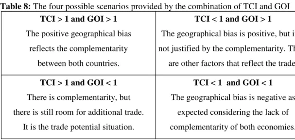
The indexes results can be combined, thus creating four possible scenarios.

Table 8: The four possible scenarios provided by the combination of TCI and GOI

Source: Castilho(2003)

On the trade potential situation one can presume that there are some obstacles that prevent the country’s export to a specific market, such as problems on the market access; Comparative advantage or other factor from another trade partner; or multinational strategies that use subcontracts.

In this case of the trade potential situation, it is advisable to investigate the tariff level or other trade barriers applied by the importer country. If there is a high level of

47_{See Castilho(2003)}

GOIi.j,a= (Xi.j,a/Xi,a) / (Mj,a/ Mw-i,a)

TCI > 1 and GOI > 1

The positive geographical bias reflects the complementarity

between both countries.

TCI < 1 and GOI > 1

The geographical bias is positive, but it is not justified by the complementarity. There

are other factors that reflect the trade.

TCI > 1 and GOI < 1

There is complementarity, but there is still room for additional trade.

It is the trade potential situation.

TCI < 1 and GOI < 1

(27)

protection, there is a good motive to negotiate trade liberalization in order to increase country exports.

It is worth pointing out that it is not possible, with this methodology, to capture the impact of the fragmentation in the production on the trade values. Therefore, the results, probably display a specialization pattern somehow unrealistic. This phenomenon is being studied by international economists and trade statisticians, which aim to develop a “new measures of trade (...) for a better understanding of the nature of cross-border trade in today’s increasingly integrated world”48. Nevertheless, this limitation is common to all methodologies in this study and in previous ones.

2.3.2. Empirical Results

The methodology applied on the following analysis is based on annual exports values, which are calculated for the 30 groups created as well as for the 4-digit level disaggregation49.It is worth pointing out that the value of world’s exports to country j is substituted by the value of country j’ imports from world, which can influence the analysis50.

Tables 9 and 10 present, respectively, the TCI and the GOI results for China between 2001 and 2009. The China’s TCI results are higher than one for several groups, being more significant for groups 19, 20 and 21. It means that China presents a higher advantage on exports to EU(15) on products as Rugs, Tulle, Padded and Textile coatings, Clothing, Footwear or similar. The GOI results are higher than one only for group 7, Ores and Metal products, between 2005 and 2008. Although only this group has a value greater than one, the remaining groups present a positive GOI, which means that the rest of China exports to the European market have not achieved their trade

potential.

According to the methodology above, the results of China’s indexes crossover are in the following table.

48

According to the” Trade Workshop: The Fragmentation of the Global Production and Trade in Value-Added – Developing New Measures of Cross Border Trade”, DECTI - World Bank in Jun 2011. More information available at the official World Bank website:

http://web.worldbank.org/WBSITE/EXTERNAL/TOPICS/TRADE/0,,contentMDK:22894003~menuPK: 2644066~pagePK:64020865~piPK:51164185~theSitePK:239071,00.html [accessed at September 2011].

49

For more information please see the Data Appendix in Annex.

50_{There is an issue on the providing data, since the database don’t have available the value of world’s}

(28)

Table 11: China’s results of the combination of TCI and GOI between the time period

2001 and 2009

The results suggest that China has trade potential in traditional products, such as Clothes and Footwear, and in more technological products, such as Tools and Brass instruments or Machinery. On other hand, the results reveal that the Comparative advantage doesn’t explain the trade between China’s and EU(15) in some Agricultural or Metal products, in Mineral Fuels, in Chemical or Medical products, in Plastic, Wood or Paper products, in Precious metals and stones, in Iron, Nickel, Zinc and similar products, or in Automobiles and other transports. For instance, the exports of these products can be in part explained by the production fragmentation51.

Considering the 4-digit level analysis, the following graph represents the China’s results of TCI and GOI for 2009. The vertical line represents the situation where TCI is equal to one and the horizontal line when GOI is equal to one. It can be seen that there is a large number of products where the trade is not explained by the complementarity of Chinese exports, which is characterized by both indexes lower than one. The trade potential situation reflects the case when GOI is lower than one and TCI is higher than one, where there are also several products in this situation. The other two possible situations don’t present a significant number of products.

51

According to Dean and Lovely(2008), the imported inputs represent about 56% of the growth in China’s exports and in 2005, about 84% of China’s intermediate inputs exports and imports were carried out by the “foreign-invested enterprises”.

TCI > 1 and GOI > 1

No Groups.

TCI < 1 and GOI > 1

No Groups, except group 7 between 2005 and 2008.

TCI > 1 and GOI < 1

Groups: 5, 12, 15, 18, 19, 20, 21, 22, 26, 27 and 30.

TCI < 1 and GOI < 1

(29)

Graph 9: Crossover of TCI and GOI for China exporst at 4-digit level in 2009

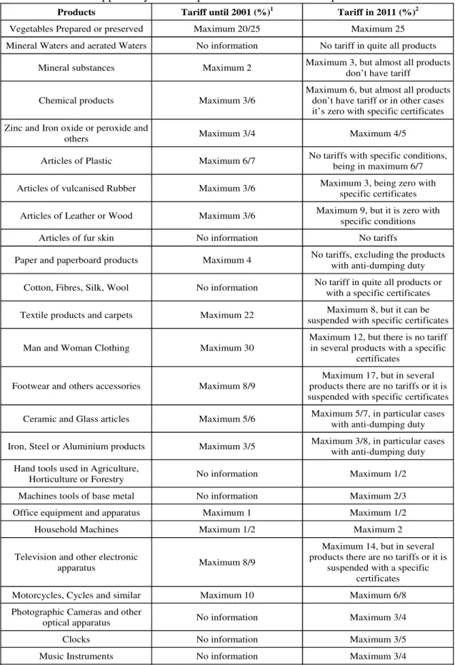
It is worth pointing out some products which present trade potential at 4-digit level: Vegetables prepared and preserved; Mineral and aerated waters; Mineral substances; Chemical products; Zinc and Iron oxide or peroxide and others; Articles of Plastic for bathrooms, kitchen or others; Articles of vulcanised Rubber; Articles of Leather or Wood; Articles of fur skin; Paper and paperboard products; Cotton, Fibres, Silk, Wool in gross; Textile products and carpets; Man and Woman Clothing; Footwear and others accessories; Ceramic and Glass articles; Iron, Steel or Aluminium products; Hand tools used in Agriculture, Horticulture or Forestry; Machines tools of base metal; Office equipment and apparatus; Household Machines; Television and other electronic apparatus; Motorcycles, Cycles and similar and their accessories; Photographic Cameras and other optical apparatus; Clocks; or Music Instruments. Some of the products in this analysis are the same that were mentioned on the indexes crossover per groups, which reinforces the results obtained in the trade potential situation.

The potential trade between China and EU(15) needs to be analysed with the

(30)

Products Tariff until 2001 (%)1 Tariff in 2011 (%)2

Vegetables Prepared or preserved Maximum 20/25 Maximum 25

Mineral Waters and aerated Waters No information No tariff in quite all products

Mineral substances Maximum 2 Maximum 3, but almost all products don’t have tariff

Chemical products Maximum 3/6

Maximum 6, but almost all products don’t have tariff or in other cases it’s zero with specific certificates Zinc and Iron oxide or peroxide and

others Maximum 3/4 Maximum 4/5

Articles of Plastic Maximum 6/7 No tariffs with specific conditions, being in maximum 6/7

Articles of vulcanised Rubber Maximum 3/6 Maximum 3, being zero with specific certificates

Articles of Leather or Wood Maximum 3/6 Maximum 9, but it is zero with _{specific conditions}

Articles of fur skin No information No tariffs

Paper and paperboard products Maximum 4 No tariffs, excluding the products _{with anti-dumping duty}

Cotton, Fibres, Silk, Wool No information No tariff in quite all products or with a specific certificates

Textile products and carpets Maximum 22 _{suspended with specific certificates}Maximum 8, but it can be

Man and Woman Clothing Maximum 30

Maximum 12, but there is no tariff in several products with a specific

certificates

Footwear and others accessories Maximum 8/9

Maximum 17, but in several products there are no tariffs or it is suspended with specific certificates

Ceramic and Glass articles Maximum 5/6 Maximum 5/7, in particular cases with anti-dumping duty

Iron, Steel or Aluminium products Maximum 3/5 Maximum 3/8, in particular cases _{with anti-dumping duty}

Hand tools used in Agriculture,

Horticulture or Forestry No information Maximum 1/2 Machines tools of base metal No information Maximum 2/3

Office equipment and apparatus Maximum 1 Maximum 1/2 Household Machines Maximum 1/2 Maximum 2

Television and other electronic

apparatus Maximum 8/9

Maximum 14, but in several products there are no tariffs or it is

suspended with a specific certificates Motorcycles, Cycles and similar Maximum 10 Maximum 6/8

Photographic Cameras and other

optical apparatus No information Maximum 3/4 Clocks No information Maximum 3/5

Music Instruments No information Maximum 3/4

Table 12: Tariffs applied by the European Union on China’s exports

Source: 1Global tariff applied by European Community in 1999-2000, according to Messerlin, P.(2002);

2_{According to European Commission Taxation in 2011, available on the website:}

(31)

Considering the information on the table above, it suggests that the tariffs applied in China’s exports have been decreased in several products. However, the values above are not sufficient to conclude that there was a decrease on the protection applied to China, since the values for 2001 are for all imports made by European Community, i.e., it is not the trade tariff applied only in China’s exports.

It is worth pointing out that “in 2006 the European Commission adopted a major policy strategy (Partnership and Competition) on China that pledged the EU to accepting tough Chinese competition while pushing China to trade fairly”52. It is negotiated the Partnership and Cooperation Agreement in 2007, which will provide “the opportunity to further improve the framework for bilateral trade and investment relations”53. Nevertheless, there are some products on the empirical analysis that present a high level of trade protection in 2011, such as Television and other electronic apparatus or Footwear and others accessories, where China need to negotiate with EU(15) to decrease the tariffs applied to its export and consequently rise its entrance on the European Market.

Regarding now the Indian case, its TCI results, as per Table 13, are higher than one for several groups, in particular for groups 19, 20 and 23. It means that India presents a superior advantage relative to EU(15) on products, such as Rugs, Tulle, Padded and Textile coatings, Clothing or Precious Metals and Stones. Indian GOI results, as per Table 14, show an index higher than one in groups 15, 19 and 21 during the time period 2001-2009, i.e., there are Indian exports to European market in products as Raw skins, Leather, Rugs, Tulle, Padded and Textile coatings or Footwear.

The results of India’s indexes crossover are in the following table.

52

According to the information available on the official website of European Commission: http://ec.europa.eu/trade/creating-opportunities/bilateral-relations/countries/china/

53_{The same source that above footnote. This agreement also includes the upgrading of the 1985}

(32)

Table 15: India’s results of the combination of TCI and GOI between the time period

2001 and 2009

The India’s results show that there is a typical case of trade with EU(15) in Raw Skins or Leather products, in Rugs, Tulle or Textile coatings, or in Clothing and Footwear. The results also suggest that India presents trade potential in several agricultural products, in Bottled or Canned products, in Ores and Metal products, in Chemical, Medical and Pharmaceutical products, in Paints, varnishes and similar products, in Silk, Wool, Cotton and similar products, in Natural stones, Porcelain or Glass products, in Precious Metals and Stones, in Iron, Steel and Copper products, or in Tools and Brass instruments. On the other hand, the results reveal that there are several products where the complementarity doesn’t explain the trade, such as Agricultural products, Waxes, Albumin and other organic substances, Natural Polymers or Modified, Rubber and its products, Plates and Plastic products, Wood, Cork and Paper products, Nickel, Aluminium, Zinc, Tin and others articles, Machinery, Automobiles and other transports, or Optical fibre, Electro-medical apparatus, Laboratory equipment and others instruments.

The following graph represents the India’s results of TCI and GOI for 2009 at 4-digit level. It shows that there is a large number of products where the trade with EU(15) is not explained by Indian specialization, since both indexes results are lower than one. The trade potential situation is given by the TCI higher than one and GOI

lower than one and it can be seen that India also presents several products in this case.

TCI > 1 and GOI > 1

Groups: 15, 19, 20 and 21.

TCI < 1 and GOI > 1

No Groups, except group 4 during the time periods 2002-2004 and 2007-2008.

TCI > 1 and GOI < 1

Groups: 1, 2, 3, 6, 7, 9, 10, 11, 13, 18, 22, 23, 24 and 26.

TCI < 1 and GOI < 1

(33)

Graph 10: Crossover of TCI and GOI for India exports at 4-digit level in 2009