UNIVERSIDADE DE LISBOA
FACULDADE DE CIÊNCIAS
DEPARTAMENTO DE ENGENHARIA GEOGRÁFICA,
GEOFÍSICA E ENERGIA
DYNAMICS AND VARIABILITY OF THE
ALONGSHORE FLOWS ON THE
NORTHWESTERN IBERIAN MARGIN
Ana Margarida Silva Pereira Teles Machado
Doutoramento em Ciências Geofísicas e da
Geoinformação
(Oceanografia)
UNIVERSIDADE DE LISBOA
FACULDADE DE CIÊNCIAS
DEPARTAMENTO DE ENGENHARIA GEOGRÁFICA,
GEOFÍSICA E ENERGIA
DYNAMICS AND VARIABILITY OF THE
ALONGSHORE FLOWS ON THE
NORTHWESTERN IBERIAN MARGIN
Ana Margarida Silva Pereira Teles Machado
Tese orientada pelo Prof. Doutor Álvaro Peliz e
pelo Prof. Doutor James C. McWilliams,
especialmente elaborada para obtenção do grau de
doutor em Ciências Geofísicas e da Geoinformação,
especialidade de Oceanografia.
2014
Acknowledgements
First, I would like to acknowledge my doctoral advisors, Álvaro Peliz and James C. McWilliams, for their scientific advice during the course of this thesis. I would also like to thank Álvaro for all the opportunities given, all that he has taught me, and for his friendship. I would like to thank James McWilliams for welcoming me to his research group at UCLA, and for guiding me in the reading course of his book, which greatly improved my knowledge of GFD.
I would also like to acknowledge my professors in Aveiro: Jesús Dubert, who introduced me to Oceanography; João Dias, for some good advices; and Yamazaki, who introduced me to linux and shell scripting. Thank you to Professora Isabel Ambar, for her encouragement, enthusiasm, and inspira-tion.
I also want to thank all my friends and colleagues in CO. A special thanks to my colleagues from the satellites room, with whom I shared ev-eryday frustrations and successes of research life; Ana Aguiar, Luisa Lamas, Filipe Neves, Dmitri Boutov. Thank you to Ana Aguiar, for reading this manuscript, and Filipe Neves for the helpful latex tips. Thank you to Sergio Abarca and Celestino Coelho for our memorable GFD discussions. I would also like to thank my colleagues at the Geology Building of UCLA, for re-ceiving me so well during my visit, and Mafalda Mascarenhas for all the administrative support in CO.
Special thanks to my friends in Aveiro, for all the good moments we’ve shared; Ana Picado, Michele Martins, Canas, Mariana, Miguel Moutinho,
Cátia Almeida, Mariana Costa. I also want to thank Jennifer Noriega for the great weekends in Venice Beach, later in Lisbon, and for the beginning of a good friendship.
This work was supported by the Portuguese Foundation for Science and Technology (FCT) under the grant SFRH/BD/40142/2007 and the projects MedEx(MARINEIRA/MAR/0002/2008) and Sflux(PTDC/MAR/100677/2008).
Quero ainda agradecer a toda a minha família e especificamente ao meu avô Orlando, pelo seu interesse no meu trabalho, e à minha tia Ana Machado, que em tempos me levou imensas vezes à praia e me transmitiu uma grande parte do gosto que tenho pelo mar.
Os principais agradecimentos são para os meus pais e para o meu irmão por sempre me apoiarem e por tudo o mais. E finalmente para o Marco, por nós, por tudo o que partilhamos, e por ser quem mais de perto sofreu as alegrias e frustrações deste percurso que é uma tese.
Abstract
This dissertation focuses on the Northwestern Iberian Margin, its seasonal and interannual variability, the vertical structure of the alongshore currents and the characteristics of the mesoscale field. These topics were explored by analyzing a 20-year simulation of the Regional Ocean Modeling System (ROMS) at 2.3 km resolution, forced by a 27 km resolution Weather Re-search and Forecast (WRF) winds (downscaled from Era-Interim reanalysis) covering the whole Western Iberian Margin. The model includes an explicit representation of the inflow/outflow at the Strait of Gibraltar in a nested grid system, and the climatological inflow of the main rivers. The model results are compared with various data. We show that currents over the slope are di-vided in three different cores: the Iberian Poleward Current (IPC), occupying the top 250 m, a deeper core at Mediterranean Water levels and in between the two, an equatorward core centered beneath the IPC core. The IPC is present almost yearlong, including in summer months, when it is close to the shelf-break and capped by the equatorward upwelling jet. After September, the IPC intensifies and its core surfaces. The main forcing mechanism of the IPC is the "Joint Effect of Baroclinicity and Relief" (JEBAR), but there is an important contribution from southerly winds in December and January, when the current is stronger and surface intensified. Regarding the inter-annual variability, we verified that the intensity of the IPC depends on the intensity of the southerly winds, from October to January. In September the intensity of the poleward flows depend on the larger scale wind stress curl, which changes JEBAR. We also show that the IPC transport has a strong variability at the synoptic scales, most of it forced by the wind. Short periods of relaxation of southerly winds are usually followed by the destabilization of the IPC and the origin of various anticyclones along the slope.
Keywords: Iberian Poleward Current, Seasonal Variability, Interannual
Resumo
A margem ocidental da Península Ibérica é uma região de grande inte-resse do ponto de vista oceanográfico devido à variedade de processos que a caracterizam e que acontecem a diferentes escalas espaciais e temporais. Na literatura esta região é particularmente conhecida por se situar no limite norte do sistema de afloramento das Canárias e por ser a região onde a Água Mediterrânica se difunde pelo Oceano Atlântico.
Neste trabalho procurou-se contribuir para o conhecimento da circulação desta região, essencialmente através do desenvolvimento e análise de uma simulação numérica do oceano, de 20 anos, que cobre o período de 1989 a 2008. A simulação foi efectuada utilizando o modelo ROMS (Regional Ocean Modeling System) (Shchepetkin and McWilliams, 2005; Shchepetkin and McWilliams, 2003; Hedstrom, 2009), com uma resolução de 2.3 km e forçado por uma atmosfera que é uma saída do modelo atmosférico WRF, com 27 km de resolução e para o mesmo período. O modelo resolve explici-tamente as trocas no Estreito de Gibraltar e inclui uma climatologia das descargas fluviais dos principais rios da região. A simulação abrange toda a Margem Ibérica Ocidental. Os resultados do modelo foram comparados com dados de temperatura da superfície do oceano e de altimetria obtidos por satélite, com uma compilação de dados de amarrações de correntómetros disponíveis para a região em estudo, e com dados de boias oceanográficas.
Assim como outras zonas limítrofes dos sistemas de afloramento, a margem ocidental da Península Ibérica apresenta uma variabilidade sazonal. O An-ticiclone dos Açores é mais intenso no Verão e geralmente encontra-se posi-cionado mais para Norte, o que juntamente com uma depressão térmica que se desenvolve sobre a Península Ibérica, resulta na persistência de ventos de norte, ao longo da margem ocidental. Os ventos de norte são favoráveis à ocorrência de afloramento costeiro e em resposta a circulação é caracterizada
por correntes para sul sobre a plataforma, água mais fria junto à costa e pre-sença de filamentos numa fase mais avançada do verão (Haynes et al., 1993; Relvas and Barton, 2002; Peliz et al., 2002). No Inverno, o Anticiclone dos Açores é geralmente menos intenso e a sua localização média situa-se mais a Sul, permitindo a passagem de vários centros de baixas pressões sobre a margem Ocidental Ibérica. Desta forma, os ventos no Inverno apresentam uma maior variabilidade à escala sinóptica, com ventos predominantes de Sul em Dezembro e Janeiro. A circulação no Inverno é dominada pela presença de uma corrente para Norte, denominada de Corrente Ibérica para o Pólo (IPC de “Iberian Poleward Current”), localizada sobre o topo da vertente e a plataforma e que transporta águas quentes e mais salgadas para Norte. Esta corrente foi descrita em vários estudos (Frouin et al., 1990; Pingree and Le Cann, 1990, 1992b; Martins et al., 2002; Peliz et al., 2005; Torres and Barton, 2006; Le Cann and Serpette, 2009). Em níveis mais profundos, a Água Mediterrânica também circula para Norte, sobre a vertente (Daniault et al., 1994). Apesar da existência de vários estudos sobre a circulação de Verão e de Inverno nesta região, ainda não é conhecido o seu ciclo sazonal, especialmente naquilo que diz respeito aos processos de transição entre Verão e Inverno e vice-versa. Um dos objectivos desta tese é fazer essa descrição.
No que diz respeito aos processos físicos que controlam a IPC, foi ex-plorada em diferentes trabalhos a forma como um gradiente meridional de densidade (que está presente ao largo da Margem continental) interage com a vertente (um gradiente zonal de profundidade acentuado), induzindo a formação de uma corrente para norte sobre o topo da vertente, com carac-terísticas semelhantes à IPC (Dubert, 1998; Peliz et al., 2003b). Outros estudos também referem a importância de episódios de vento de sul, associa-dos a eventos em que uma corrente superficial para norte é particularmente intensa (Le Cann and Serpette, 2009). Para compreender a importância rela-tiva destes dois processos (vento e estrutura interna da densidade) é realizada uma análise da variação sazonal dos balanços de vorticidade sobre a vertente. A IPC apresenta uma grande variabilidade inter-anual, como foi
demons-trado por vários estudos que a analisaram com base na temperatura da super-fície do oceano obtida por satélite (Garcia-Soto et al., 2002; Peliz et al., 2005; Le Cann and Serpette, 2009; Garcia-Soto and Pingree, 2011). Neste trabalho é feita uma descrição da variação inter-anual da intensidade da IPC e dos seus efeitos nos campos de temperatura e salinidade. São também analisados os vários mecanismos que podem controlar a variabilidade inter-anual.
Na bibliografia são descritos vários episódios de formação de turbilhões, resultantes da destabilização da IPC. Estes vórtices têm polaridade anti-ciclónica e contêm no seu núcleo águas mais quentes e de maior salinidade do que as águas circundantes. Estes anticiclones, foram observados pela primeira vez na costa Norte da Península Ibérica por Pingree and Le Cann (1992b), que os denominaram de “Swoddies” – “Slope Water Oceanic Eddies”. Estru-turas semelhantes a estas também foram observadas na costa Oeste (Fiúza et al., 1998; Oliveira et al., 2004; Peliz et al., 2003b, 2005). Dubert (1998) and Peliz et al. (2003b) estudaram a formação de Swoddies em simulações numéricas idealizadas e demonstraram que a topografia tem um papel impor-tante para o desenvolvimento das instabilidades que dão origem aos vórtices, e que estes geralmente se formam a seguir aos principais acidentes topográ-ficos. Neste trabalho procurou-se perceber as suas condições de formação, bem como fazer uma estatística das características da sua população.
Os resultados confirmaram que a corrente sobre a vertente é composta por 3 estruturas distintas: a IPC ocupa os 250 m superficiais; as profundidades de ∼600-1200 m são ocupadas por uma corrente mais profunda também para norte, aos níveis da Água Mediterrânica; e entre as duas, sob o centro da IPC, desenvolve-se uma contra-corrente para sul. Verificou-se que a IPC está presente durante praticamente todo o ano, incluindo nos meses de Verão. No Verão a IPC é sub-superficial e o seu máximo de intensidade localiza-se junto ao bordo da plataforma, debaixo do jacto de afloramento que ocupa a região da plataforma. A partir de Setembro, a IPC intensifica-se e torna-se máxima à superfície.
a partir da qual se concluiu que o mecanismo forçador da IPC mais impor-tante é o JEBAR (de “Joint Effect of Baroclinicity and Relief” ou “Efeito Conjunto de Baroclinicidade e Topografia”), associado à presença de gradi-entes meridionais de densidade. A IPC tem uma forte componente advectiva e transporta águas menos densas para norte, caracterizadas por temperaturas e salinidades mais elevadas, diminuindo os gradientes meridionais de densi-dade sobre a vertente, e desta forma, diminuindo a intensidensi-dade do JEBAR e a sua importância enquanto processo que acelera a corrente. Verificou-se que também existe uma contribuição importante dos ventos de sul, princi-palmente em Dezembro e em Janeiro, quando a corrente está mais intensa e intensificada junto à superfície.
O modelo reproduz os anos anómalos da IPC em fase com a realidade. Os resultados demonstraram que entre Outubro e Janeiro existe uma relação linear entre médias mensais da intensidade da IPC e as médias mensais da in-tensidade de ventos de sul. Em Setembro, a inin-tensidade da corrente depende do campo do rotacional do vento sobre uma região maior, que ao alterar a es-trutura do campo de densidades e o gradiente meridional de densidade, altera o valor do JEBAR que é o principal factor que controla a IPC em Setem-bro. Verificou-se também que em geral, quanto mais forte a corrente, mais intensas são as anomalias de temperatura e salinidade obtidas. No entanto, os fluxos de calor locais e os balanços de precipitação/evaporação, também são importantes, especialmente em alguns anos anómalos.
Por fim é demonstrado que a IPC tem uma forte variabilidade à escala sinóptica, maior parte da qual é forçada pela variabilidade do vento. A IPC destabiliza-se, principalmente, perto de variações topográficas acentuadas, dando origem à formação de anticiclones denominados de Swoddies. Estes formam-se constantemente, mas é em períodos de relaxamento de vento de sul que se verificam as maiores taxas de formação. Após o relaxamento dos ventos, a corrente apresenta sinais de instabilidades, que posteriormente crescem e dão origem aos anticiclones. Os Swoddies interagem com outros vórtices, particularmente com ciclones intensificados em profundidade, e a
interacção resulta numa propagação para o largo, e no transporte de águas mais quentes e mais salgadas da IPC para o oceano aberto.
Palavras-chave: Corrente Ibérica para o Pólo, Ciclo Sazonal, Variabilidade Inter-Anual, Turbilhões, Modelo Oceânico, Swoddies
Contents
List of Acronyms and Abbreviations v
List of Figures vii
Introduction 1
1 Model Configuration and Observed Data 5
1.1 Model configuration . . . 5
1.1.1 Model . . . 5
1.1.2 Climatological Simulation . . . 6
1.1.3 Two-way nesting simulation . . . 7
1.1.4 Atmospheric Forcing . . . 8
1.1.5 Rivers and Mediterranean Outflow . . . 9
1.1.6 Spin-up . . . 10
1.2 Observed data . . . 10
1.3 Comparison of model results with observations . . . 12
2 Seasonal Cycle of the IPC and other Alongshore Flows 19 2.1 Introduction . . . 19
2.2 Seasonal currents . . . 20
2.2.1 Horizontal circulation . . . 20
2.2.2 Vertical structure of the alongshore currents . . . 24
2.3 Surface eddy kinetic energy . . . 37
2.4 Temperature and Salinity . . . 39 i
ii CONTENTS
2.4.1 Heat and Salt Budgets . . . 42
2.5 Discussion and Conclusions . . . 47
3 Seasonal Forcing of the Slope Currents 51 3.1 Introduction . . . 51
3.2 Depth-averaged vorticity equation . . . 52
3.3 Time-mean balance . . . 55
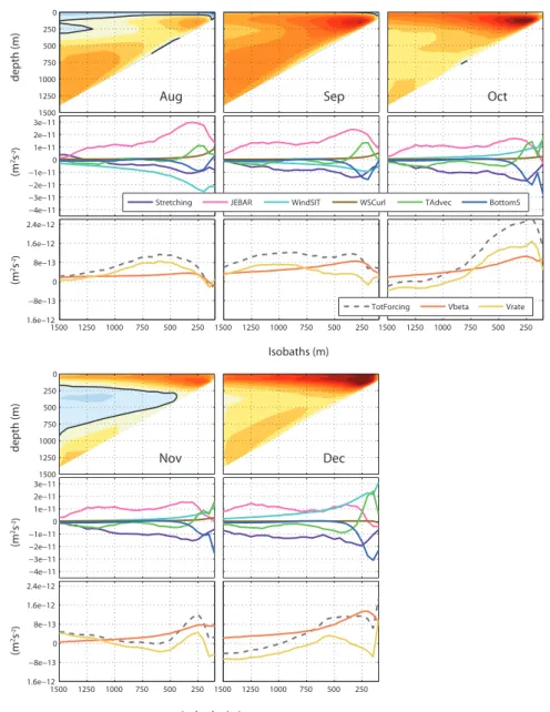
3.4 Seasonal cycle of integrated vorticity terms . . . 56
3.5 Flow structure . . . 59
3.6 Discussion and Conclusions . . . 64
4 Interannual Variability of the Iberian Poleward Current 67 4.1 Introduction . . . 67
4.2 Comparison of model results with previous studies . . . 68
4.3 Description of the Interannual variability . . . 69
4.3.1 Year-to-year IPC changes . . . 72
4.3.2 Variability of the Forcing of the IPC . . . 80
4.4 Discussion and Conclusions . . . 86
5 Swoddies 91 5.1 Introduction . . . 91
5.2 Methods . . . 93
5.2.1 Eddy Tracking Algorithm . . . 93
5.2.2 Eddy tracking at 100 and 250 m depths . . . 93
5.3 Statistics of detected eddies . . . 95
5.3.1 Different Eddies in Depth and the Statistics of Vorticity 95 5.3.2 Characteristics of the Surface and Mid-Water Eddies . 97 5.4 Swoddies: Slope Water Eddies on the Winter Season . . . 102
5.4.1 Comparisons with observations . . . 102
5.4.2 Description of the 1989/1990 strong IPC Winter . . . . 108
5.4.3 Swoddies birth-rate time series . . . 114
CONTENTS iii
5.4.5 Swoddies sizes . . . 120 5.5 Discussion and Conclusions . . . 122
Conclusions 127
List of Acronyms and
Abbreviations
COADS Comprehensive Ocean-Atmosphere Data Set CT D Conductivity, Temperature, and Depth sonde EKE Eddy Kinetic Energy
EN ACW Eastern North Atlantic Central Water
EN ACW st Eastern North Atlantic Central Water of Sub-Tropical origin GF D Geophysical Fluid Dynamics
GHRSST Group for High Resolution Sea Surface Temperature IP C Iberian Poleward Current
IP SU Iberian Poleward Slope Undercurrent JEBAR Joint Effect of Baroclinicity and Relief M eddies Mediterranean Water eddies
N AO North Atlantic Oscilation RM Se Root Mean Square Error
ROM S Regional Ocean Modeling System v
vi List of Acronyms and Abbreviations
SLA Sea Level Anomaly SSH Sea Surface Height
SSHa Sea Surface Height anomaly SST Sea Surface Temperature
Swoddies Slope Water Oceanic eDDIES U SCC Upper Slope Countercurrent
W RF Weather Research and Forecast Model W SC Wind Stress Curl
List of Figures
1.1 Maps showing the 3 spatial domains used in the model con-figuration. . . 6 1.2 Time-depth distribution of all the current meter data available. 11 1.3 Model - Data comparisons. . . 13 1.4 Taylor diagram of model data comparisons. . . 14 1.5 Average seasonal cycle of model and satellite SST. . . 16 1.6 Time series of anomalies, after removing the seasonal signal
presented in Fig. 1.5. . . 16 1.7 December averaged model and satellite SST fields. . . 17 2.1 Map with sections and positions of current meter observations. 22 2.2 Monthly mean fields of the depth-averaged velocity for the top
500 m. . . 23 2.3 Hovmoller diagrams of SSHa. . . 24 2.4 Percentage (%) of standard deviation relative to seasonal and
6 month variability of alongshore currents. . . 26 2.5 Section I - Vertical sections of the monthly averages of 20-years
simulation of alongshore velocities (m s−1) . . . 29 2.6 Section II - Vertical sections of the monthly averages of
20-years simulation of alongshore velocities (m s−1) . . . 30 2.7 Section III - Vertical sections of the monthly averages of
20-years simulation of alongshore velocities (m s−1) . . . 30 vii
viii LIST OF FIGURES
2.8 Section I - Comparison of alongshore currents from current meter monthly averages and model. . . 32 2.9 Section II - Comparison of alongshore currents from current
meter monthly averages and model. . . 33 2.10 Section III - Comparison of alongshore currents from current
meter monthly averages and model. . . 34 2.11 Seasonal cycle of the meridional transport across different
ar-eas and for sections I, II, III. . . 36
2.12 Hovmoller diagrams of EKE (cm2
s−2) at 20 m depth. . . 39 2.13 Average seasonal cycle of temperature and salinity. . . 41 2.14 Monthly average vertical sections of meridional velocities
to-gether with temperature and salinity. . . 42 2.15 Global averaged heat and salt fluxes for April, July, October
and December. . . 44 2.16 Average seasonal cycle of volume averaged (top 200 m) heat
and salt budgets for northern and western coast. . . 46 2.17 Schematic representation of the seasonal cycle of the
along-shore currents. . . 48 3.1 Map with area to compute integrated vorticity budgets. . . 55 3.2 Seasonal cycle of area-integrated values of all terms in vorticity
equation. . . 57 3.3 August to December cross-structure monthly means. . . 60 3.4 August to January monthly means vertical sections at 42.2◦N. 63 3.5 Mean meridional density gradient obtained in section V. . . . 64 4.1 Time series of anomalies, after removing the seasonal signal
presented in Fig. 2.13. . . 71 4.2 Vertical sections of meridional velocities and temperature. . . 73 4.3 Vertical sections of meridional velocities and salinity. . . 74 4.4 Cumulative time integral of the anomalies of volume averaged
LIST OF FIGURES ix
4.5 Diagrams of monthly averages of various quantities. . . 81 4.6 September mean fields. . . 83 4.7 Area averaged salinity represented in function of depth and
time. . . 89 5.1 Distribution of eddies formed at the slope area from October
to March. . . 94 5.2 Probability density function (PDF) and skewness of vorticity
fields in the slope area. . . 96 5.3 Total number of eddies formed on the slope area in each month. 97 5.4 Maps with density of eddies formation. . . 98 5.5 Average vertical profiles of salinity, temperature and vorticity,
of different eddies populations. . . 100 5.6 Trajectories of eddies tracked for a minimum of 2 months. . . 101 5.7 Comparison between model and satellite SST for various days
from the winter 1989/1990. . . 104 5.8 Comparison between model and satellite SST for various days
from the winter 1995/1996. . . 105 5.9 Comparison between model and satellite SST for various days
from the winter 2006/2007. . . 106 5.10 Comparison between model and satellite SST for various days
from different winters. . . 107 5.11 Swoddies in the winter of 1989/1990 (1). . . 110 5.12 Swoddies in the winter of 1989/1990 (2). . . 111 5.13 Swoddies in the winter of 1989/1990 (3). . . 112 5.14 Evolution in time of the area averaged wind. . . 113 5.15 Time series of wind, transport and Swoddies formation. . . 115 5.16 Trajectories of 2 Swoddies that were tracked for longer than a
year. . . 116 5.17 Zonal sections of temperature, salinity and density, for
x LIST OF FIGURES
5.18 Zonal sections of temperature, salinity and density, for differ-ent dates. . . 119 5.19 Eddies first month average profiles of salinity, temperature and
vorticity. . . 120 5.20 Histograms of eddies radius. . . 121 5.21 Power spectrum of the EKE. . . 122
Introduction
The Western Iberian Margin is very interesting for the variety and complexity of the processes that take part simultaneously, at different temporal and spa-tial scales. It is famous for two main reasons. In one hand it is the northern-most limit of the Canary Upwelling System, and, on the other hand, it is the place where the Mediterranean Water overflows into the Atlantic. Near the surface, during the summer period, the circulation is upwelling-type, charac-terized by equatorward shelf flows, cold water fronts and filaments (Haynes et al., 1993; Relvas and Barton, 2002; Peliz et al., 2002). This happens be-cause the Azores High Pressure Cell is stronger and displaced northwards in summer, resulting in persistent northerly and upwelling favorable winds. In winter, the Azores High Pressure Cell weakens and moves southwards, allowing the passage of various winter atmospheric cyclones over the West-ern Iberian Margin. This results in a more variable wind, predominantly southerly in December and January. The ocean circulation in the winter is dominated by the Iberian Poleward Current (IPC), flowing over the upper slope and outer shelf of the Western Iberian Margin and extending all along to the northern coast of the Iberian Peninsula. This current was described in various studies (Frouin et al., 1990; Pingree and Le Cann, 1990, 1992b; Martins et al., 2002; Peliz et al., 2005; Torres and Barton, 2006; Le Cann and Serpette, 2009).
Dubert (1998) and Peliz et al. (2003b), amongst others, showed that the presence of a meridional density gradient interacting with the slope, as hap-pens in the Western Iberian Basin, can give origin to a surface intensified
2 Introduction
poleward current over the slope, with similar characteristics to the observed IPC. Other authors believe southerly winds are also important for the de-velopment of surface intensified events of the IPC (Le Cann and Serpette, 2009).
Analysis of satellite SST data suggest that the IPC is subjected to a strong interannual variability. Various studies focused on these year-to-year changes in winter SST anomalies to infer about the interannual variability of the current (Garcia-Soto et al., 2002; Peliz et al., 2005; Le Cann and Serpette, 2009; Garcia-Soto and Pingree, 2011). However, it is not clear what forces the year-to-year variability of the IPC intensity and its response in terms of temperature and salinity anomalies.
The IPC is known to destabilize, and give origin to anticyclonic eddies that carry the warmer and saltier water offshore. These eddies were first identified on the northern coast by Pingree LeCann 1992a, who named them by ’Slope Water Oceanic eDDIES’ (Swoddies). They were also observed on the western coast (Fiúza et al., 1998; Oliveira et al., 2004; Peliz et al., 2003b, 2005). Dubert (1998) and Peliz et al. (2003b) studied their formation using idealized model simulations, and showed that topography is important for the formation of the eddies, with their places of formation being usually located downstream of topographic accidents.
Despite the existence of many observational and modeling studies of this region, there are still many unanswered questions regarding the seasonal cycle of the IPC, its interannual variability, and its destabilization and formation of eddies. An extended introduction to each of these problems is included in the beginning of each chapter. We developed a regional ocean simulation, focusing on the period from 1989 to 2008, and used it together with the available in-situ and satellite observations, to study this region with further detail and address some of the open questions.
This thesis is organized as follows:
In Chapter 1, is presented a description of the model, of the simulations and an introduction to the various datasets used. Comparisons between the
Introduction 3
model and observations are presented.
Chapter 2 provides a characterization of the vertical structure of the mean alongshore flow and its mean seasonal variability.
In Chapter 3, the main mechanisms forcing the IPC are investigated, and their seasonal variability is analyzed.
In Chapter 4, the interannual variability of the IPC is described, and the mechanisms driving its variability are investigated.
Chapter 5 presents a study of the formation of anticyclonic eddies (Swod-dies) associated with the destabilization of the IPC. It makes a characteriza-tion of their populacharacteriza-tion and analyses some events of formacharacteriza-tion.
Finally, a summary of main conclusions is presented along with newly raised questions.
Chapter 1
Model Configuration and
Observed Data
1.1
Model configuration
1.1.1
Model
The Regional Ocean Modeling System (ROMS), is a primitive equation, hydrostatic, sigma coordinate, free-surface ocean model (Shchepetkin and McWilliams, 2005; Shchepetkin and McWilliams, 2003; Hedstrom, 2009). The need for solving processes at a wide range of horizontal spatial scales led us to choose the ROMS-AGRIF version (http : //www.romsagrif.org/), because of its nesting capabilities [Penven et al. (2006) and Debreu et al. (2012)].
ROMS uses a third-order upstream momentum and tracers advection scheme, which is dissipative in nature, allowing a simulation without ex-plicit viscosity or diffusivity. The subgrid-scale vertical mixing processes in the interior and in the boundary layers are parametrized with a K-profile parametrization scheme (Large et al., 1994).
This model configuration was developed in two phases. The first, was a large scale climatological simulation using the large domain represented in
6 1. Model Configuration and Observed Data
Fig. 1.1 (grid C0), to produce equilibrium solutions for initialization and boundary conditions. The second phase consists of a high resolution 2-way nested realistic simulation (domains represented in Fig. 1.1 – grids A0 and A1), initialized and forced on the boundaries by the outputs of the climato-logical run. 40oW 30oW 20oW 10oW 0o 24oN 30oN 36oN 42oN 48oN grid C0 grid A0 grid A1 12oW 11oW 10oW 9oW 8oW 7oW 6oW 38oN 39oN 40oN 41oN 42oN 43oN 44oN I II III Douro Tejo Cavado Lima Minho Ave Rias1 Rias2 Mondego 1 2 3 W N
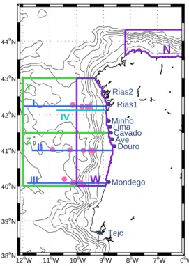
Figure 1.1: On the left: Map showing the 3 spatial domains used in the model con-figuration (Grids C0, A0 and A1). On the right: a zoom on the coastal margin we are focusing on. The name of the rivers considered in the simulation are indicated. (1-3) blue dots represent the position of 3 moored buoys located at 9.43W 42.12N, 9.21W 43.50N and 7.67W 44.12N; (N,W) purple boxes represent 2 domains, on northern and western coasts; the pink dots represent the current meter observa-tions; the black contours represent the isobaths of 100, 200, 500, 1000, 2000, 3000, 4000 and 5000 m.
1.1.2
Climatological Simulation
For the domain C0, we made a 10 years simulation, with horizontal grid reso-lution of 1/10◦, which corresponds to approximately 7.5 km near the northern boundary and 10 km in the south. This results in an horizontal grid with 449x311 cells. In the vertical direction, the grid has 32 levels with enhanced resolution near the surface (the surface stretching parameter is θS = 6 and
1.1 Model configuration 7
the bottom stretching parameter θB = 0) to better resolve the boundary layer everywhere in the domain. The baroclinic time step is 1080 seconds. The model grid, forcing, initial and climatology files were built using the ROM-STOOLS package (Penven et al., 2008). The topography was derived from database ETOPO2 (National Geophysical Data Center – NDGC), smoothed and interpolated to the model grid. The model was initialized with Levitus climatology (WOA05 – Locarnini et al. (2006) and Antonov et al. (2006)) in January. Along the open boundaries it was used a modified radiation boundary condition together with a flow adaptive nudging to the Levitus climatology (Marchesiello et al., 2001; Locarnini et al., 2006; Antonov et al., 2006). The nudging is stronger in case of inflow in the open boundaries and weaker in case of outflow, respectively with time scales of 1 day and 1 year for tracers, and 10 days and 1 year for momentum. Regarding the external forcing, the momentum, heat and freshwater fluxes were extracted from the Comprehensive Ocean-Atmosphere Data Set (COADS) monthly climatology at 1/2◦ resolution (da Silva et al., 1994). The Mediterranean Water is forced in the model using a nudging term that prevents the divergence of the model solution from the Levitus climatology. The nudging condition implemented is described in Peliz et al. (2007). After a spin-up of around 2 years, the volume averaged kinetic energy of the simulation reaches an equilibrium (not shown). Years 4 to 7 of this simulation were used to create a monthly climatology for the high resolution domains A0 and A1 (see Fig. 1.1).
1.1.3
Two-way nesting simulation
This simulation uses a larger domain (represented as A0 in Fig. 1.1) and an embedded child domain (represented as A1 in Fig. 1.1), running simul-taneously and exchanging information between each other at every model time-step. A0 spans from 33◦N to 46◦N and 18◦W to 1◦W, with an hori-zontal resolution within the range of 6.4 to 7.8 km (205x205 grid cells). A1 spans from 34.8◦N to 45.0◦N and 13.6◦W to 3.4◦W, with horizontal resolu-tion from 2.2 to 2.5 km (368x482 grid cells). In the vertical, the grids have
8 1. Model Configuration and Observed Data
40 levels with enhanced resolution near the surface (θS = 6 and θB = 0) to better resolve the boundary layer everywhere in the domain. The baroclinic time steps are 900 seconds and 300 seconds for grids A0 and A1, respec-tively. The model grids were also built using the ROMSTOOLS package (Penven et al., 2008). The topography was derived from Scripps Institution for Oceanography global topography (Smith and Sandwell, 1997) and from Spanish data for the Strait of Gibraltar (Sanz et al., 1991). The merged to-pography was smoothed to avoid pressure gradient errors, so that the slope parameter (Beckmann and Haidvogel, 1993) is everywhere lower than 0.19.
Radiation condition plus flow adaptive nudging towards a monthly cli-matology, were used along A0 open boundaries (Marchesiello et al., 2001). The monthly climatology was created from the outputs of the climatological simulation. No interannual variability is introduced to the domain from the open ocean, through the open boundaries.
Null viscosity and diffusivity were used everywhere, except in a sponge layer of 15 km width along the open boundaries of domain A0 (see Fig. 1.1). Increased values of viscosity and diffusivity were applied in the Gulf of Cadiz near the Strait of Gibraltar to produce a more realistic representation of the Mediterranean Undercurrent (Peliz et al., 2012) and near the mouth of river inputs, to represent more realistic water mass characteristics of the river plumes. In the sponge layer, the viscosity increases smoothly from zero in the interior to 300 m2
s−1 in the boundary.
1.1.4
Atmospheric Forcing
The atmospheric forcing was created using the outputs of a Weather Research and Forecast (WRF) model simulation, covering the period from 1989 to 2008 with hourly outputs and with horizontal resolution of 27 km (Soares et al., 2012). The variables used were the wind at 10 m, the temperature and the specific humidity at 2 m, the precipitation, the short wave net radiation and incident long wave radiation. The fluxes of momentum and sensible and latent heat, are computed internally in the ocean model at each time step,
1.1 Model configuration 9
using a bulk formulation [Fairall et al. (1996) and Liu et al. (1979)]. The upward long wave radiation is also computed internally in the model, using the Stefan-Boltzmann law with the computed sea surface temperature (SST).
1.1.5
Rivers and Mediterranean Outflow
The rivers that discharge a significant amount of fresh water to the coastal ocean are Tejo, Mondego, Douro, Ave, Cávado, Lima, Minho, together with smaller ones that discharge into the Galician Rias (Tambre, Ulla, Umia, Lérez and Verdugo) (subplot on the right in Fig. 1.1) and Guadalquivir. Due to recurrent and extensive gaps in river outflow data, we used climatologies of river discharges based on the adjusted seasonal cycle. We used the analyt-ical adjustments to simulate the runoff in the model. For the northwestern Iberian rivers we used data from Otero et al. (2010) (Douro River was the southernmost one considered in this study). Runoff data for Mondego and Tejo Rivers were obtained from Chainho et al. (2006) and Neves (2010), re-spectively. Guadalquivir is not shown in Fig. 1.1 because it is out of the zoom area represented on the plot on the right, but it was considered in the simulation and introduced the same way as in Peliz et al. (2012).
To get realistic values for the salinity of the river plumes it was necessary to increase mixing near the river mouths. In nature, many of these rivers discharge in estuaries where the fresh water is strongly mixed with sea wa-ter, due to tide effects, strong currents and atmospheric heat forcing. All of these processes increase the mixing of the river plumes with the coastal ocean, modifying the salinity and density of the plumes. Because of their reduced size, the estuaries are not resolved with the horizontal resolutions used in this simulation. To represent the unresolved mixing processes, we used a constant velocity profile for the outflow of the rivers, instead of the exponential one (with velocity increasing to the surface). Using this type of profile, freshwater is introduced near the bottom, forcing vertical convection and consequently vertical mixing. We also introduced a circular region with increased horizontal diffusion near the mouth of all the rivers, whose radius
10 1. Model Configuration and Observed Data
and intensity vary in time, proportionally to the intensity of the river outflow. To guarantee a realistic Mediterranean outflow, we used the same proce-dure as in Peliz et al. (2012).
1.1.6
Spin-up
A spin-up of 2 years was done, already taking in consideration the rivers and mediterranean outflow as described. The atmospheric forcing, momentum, heat and freshwater fluxes were from the Comprehensive Ocean-Atmosphere Data Set (COADS).
After the spin-up, the model ran for 20 years, 1989 to 2008, which is the period analyzed in this paper.
1.2
Observed data
We compare the model results with currents, temperature and salinity time-series measured at 3m depth, at the buoys of the Spanish Public Agency of Marine Affairs, Puertos del Estado (http://www.puertos.es/en). Figure 1.1 shows the positions of the buoys Villano Sisargas, Estaca Bares and Cabo Silleiro, represented respectively as 1, 2 and 3.
We also used altimeter products, produced by Ssalto/Duacs and dis-tributed by Aviso, with support from Cnes (http://www.aviso.oceanobs. com/duacs/). The maps have a spatial resolution around 28 km and a time resolution of one week.
To compare with the model sea surface temperature (SST), we used satel-lite AVHRR Pathfinder Version 5.2 (PFV5.2) data, obtained from the US National Oceanographic Data Center and GHRSST (http://pathfinder. nodc.noaa.gov) (Casey et al., 2010).
We also used data from a set of historical moored current meter data from 1984 to 1995. The data were collected in the frame of different projects (CORPAC, MORENA, Bord-Est1 and MEDPOR) and are described in Am-bar (1985), AmAm-bar and Fiúza (1994), Daniault et al. (1994) and Frouin et al.
1.2 Observed data 11
(1990). Most of the available data was from one of the 3 sections repre-sented in Fig. 1.1 (I, II and III). The pink dots in the same figure represent the distribution of the available current meter moorings. The depths of the current meters are shown in the first subplot of Figures 2.5, 2.6 and 2.7, re-spectively for sections I, II and III. The time/depth distribution of the data is represented in Fig. 1.2. Data from the different sections are represented in different colors. We have a total of 11000 days of observations distributed over the various sections, depths and times. There are a total of 2520 days of observations in section I, 4981 days in section II and 3498 days in section III. We use all the available data to compute monthly averages for each of the current meter locations. We present the comparisons between the average seasonal cycle of currentmeter data and the model in chapter 2.
83 84 85 86 87 88 89 90 91 92 93 94 95 −1400 −1200 −1000 −800 −600 −400 −200 0 years depth(m) sec I − 2520 days sec II − 4981 days
sec III − 3498 days
Figure 1.2: Time-depth distribution of all the current meter data available. Data from the different sections (I, II, III) (represented in figure 1.1) is plotted with different colors. The inset shows the total number of days of data available in each section.
12 1. Model Configuration and Observed Data
1.3
Comparison of model results with
observa-tions
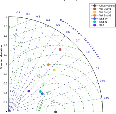
To compare the model results with the observations, we plot time series of monthly averages of different variables, for the model and the observations (Fig. 1.3). To summarize the model-observations comparisons the variables are plotted in a normalized Taylor diagram (Taylor, 2001) (Fig. 1.4). The Taylor Diagram shows the standard deviation of model and observations, the root mean square (RMS) error of the model, and the correlation coefficient between model and observations. The closer the model point is to the ob-servations point, the better the model reproduces obob-servations. To allow the comparison between the different quantities, model RMS and standard devi-ation of both model and observdevi-ations were divided by the standard devidevi-ation of the observations.
The model velocity data were interpolated to the depth, latitude and longitude of each buoy. Figure 1.3 a, b and c, presents the comparisons for buoy 1, 2 and 3, respectively. The velocity components for locations of buoys 1 and 2 were rotated to the direction of maximum variance (approximately alongshore). In the case of buoy 3, the direction of maximum variance is coincident with the zonal component (less than 1◦ difference) and the zonal component is presented instead. The available time series start in 1998. There are discrepancies in some years, the clearest ones for buoy 1 in the end of 2003 and for buoy 3 in the end of 2001. We find a better comparison between the model and the velocity measured at buoy 2, with a correlation coefficient of about 0.75 (see Fig. 1.4). The model correlation with buoys 1 and 3 alongshore velocity is around 0.65. All the correlations are significant at 1% level. Despite these differences, the model reproduces the main observed variability with a high realism given the fact that no data assimilation is used.
1.3 Comparison of model results with observations 13 1993 1994 1995 1996 1997 1998 1999 2000 2001 2002 2003 2004 2005 2006 2007 2008 2009 −0.1 −0.05 0 0.05 0.1 0.15 d
model sla altim sla
1989 1990 1991 1992 1993 1994 1995 1996 1997 1998 1999 2000 2001 2002 2003 2004 2005 2006 2007 2008 2009 35.2 35.4 35.6 35.8 36 36.2 salt(PSU) e 1989 1990 1991 1992 1993 1994 1995 1996 1997 1998 1999 2000 2001 2002 2003 2004 2005 2006 2007 2008 2009 35 35.2 35.4 35.6 35.8 36 salt(PSU) f 1998 1999 2000 2001 2002 2003 2004 2005 2006 2007 2008 2009 −0.4 −0.2 0 0.2 0.4 u rot(m s −1 ) a 1998 1999 2000 2001 2002 2003 2004 2005 2006 2007 2008 2009 −0.4 −0.2 0 0.2 0.4 u rot(m s −1 ) b 1998 1999 2000 2001 2002 2003 2004 2005 2006 2007 2008 2009 −0.4 −0.2 0 0.2 0.4 u(ms −1 ) c sla(m)
Figure 1.3: Model (blue) – Data (red) comparisons. (a-c) alongshore velocity in buoys 1-3 (see buoys position in Fig. 1.1); (d) sea level anomalies, spatial averaged in domain W (see domain in Fig. 1.1); (e-f ) salinity in buoys 1-2.
14 1. Model Configuration and Observed Data 0.2 0.4 0.6 0.8 1 1.2 1.4 1.6 1.8 2 0 0.2 0 0.4 0 0.6 0 0.8 0 1 0 1.2 0 1.4 0 1.6 0 1.8 0 2 0.1 0.2 0.3 0.4 0.5 0.6 0.7 0.8 0.9 0.95 0.99 Standard deviation C o rr e l a t i o n C o e f f i c i e n t R M SD
Normalized Taylor Diagram
Observations Vel Buoy1 Vel Buoy2 Vel Buoy3 SST W SST N SLA
Figure 1.4: Taylor diagram of model data comparisons. Comparison of all vari-ables plotted in Fig 1.3 except salinity.
The salinity comparisons are presented in Fig. 1.3 e and f, for buoys 1 and 2, respectively. Buoy 3 is not represented because there are few data available, very noisy and with many gaps. In some periods, there is a good comparison, as for example in buoy 1 from the beginning of 2006 till the middle of 2007, and in buoy 2 from beginning of 2004 till the beginning of 2006. But in other periods the comparison is bad. It seems that the model is not reproducing the low salinity anomalies, that might be associated with anomalous river discharges and intense river plume events not simulated be-cause the model river discharge is climatological. Nevertheless, some failures and problems in the salinity sensors may not be excluded either, since these larger differences usually precede periods of missing data.
Model sea surface height is compared with altimetry data from AVISO (Fig. 1.3 d). Both model and AVISO data were horizontally averaged within
1.3 Comparison of model results with observations 15
domain W (Fig. 1.1). The steric effect was added to the model solution (as in Peliz et al. (2013)), so that the comparison is possible. The model reproduces correctly the seasonal cycle and part of the interannual variability, but the covariance of both time series is not always good. The statistics of the comparison are represented in the Taylor Diagram (Fig. 1.4). The correlation between altimetry data and model is 0.7, significant at 5% level.
We also used satellite SST to compare with model SST for the northern and western coasts: we compare horizontal averages in domains N and W (Fig. 1.1), and will name it respectively, SSTN and SSTW. The model reproduces the average seasonal cycle (see Fig. 1.5 for SSTN and SSTW). In winter, the model SST is around 0.5◦C higher than the observations, and in summer, it is around 0.5◦C colder, on both the northern and the western coasts. This difference can be associated with a deficient parameterization of the mixing processes, or the surface heat fluxes. To compare the interannual variability of the SST anomalies, we computed the monthly means of the horizontal averaged SSTN and SSTW and removed the respective seasonal cycle. The interannual anomalies are well reproduced in the model (Fig. 1.6 for SSTN and SSTW). The statistics of these comparisons are represented in the Taylor Diagram (Fig. 1.4). In the case of the SST, we compare the time series after removing the seasonal cycle of both model and satellite data, since the seasonal cycle explains most of the variability of the SST. The correlation between model and satellite SST anomalies is between 0.8 and 0.9 (Fig. 1.4) for both the northern and western coasts (around 0.95 if the seasonal cycle is not removed). The correlations are significant at 1% level.
We plot the averaged December SST fields from model and satellite from 1989 to 2008 (Fig. 1.7), for comparison. The model fields were computed by averaging the entire month, while satellite images were computed by av-eraging the available cloud free data for each pixel, so they are not exactly same. The missing data in the satellite SST fields means that there was not any cloud free image on that month. Despite these differences, it is visible that the model captures the main observed interannual variability.
16 1. Model Configuration and Observed Data 12 14 16 18 20 22 Domain N SST W ( oC) months J F M A M J J A S O N D 12 14 16 18 20 22 months SST W ( oC) Domain W SST−roms SST−pathfinder
Figure 1.5: Average seasonal cycle: (a) model and satellite SST averaged in domain N (see Fig. 1.1); (b) the same as (a), but for domain W.
−2 −1 0 1 2 SSTa N ( oC)
Domain N SST−roms SST−pathfinder
1989 1990 1991 1992 1993 1994 1995 1996 1997 1998 1999 2000 2001 2002 2003 2004 2005 2006 2007 2008 2009 −2 −1 0 1 2 SSTa W ( oC) Domain W SST−roms SST−pathfinder
Figure 1.6: Time series of anomalies, after removing the seasonal signal presented in Fig. 1.5. (a) model and satellite SST averaged in domain N (see Fig. 1.1); (b) the same as (a), but for domain W.
1 .3 Co m p a r is o n o f m o d e l re s u lt s w it h o b s e r v a ti o n s 17 18 1989 1990 1991 1992 1993 1994 1995 1996 1997 1998 1999 2000 2001 2002 2003 2004 2005 2006 2007 2008 (a) 13 14 15 16 17 18 1989 1990 1991 1992 1993 1994 1995 1996 1997 1998 1999 2000 2001 2002 2003 2004 2005 2006 2007 2008 (b)
Chapter 2
Seasonal Cycle of the IPC and
other Alongshore Flows
2.1
Introduction
The Western Iberian Margin is characterized by persistent, multicore sea-sonally varying flows. The summer is dominated by upwelling-type shelf cir-culation with associated equatorward currents, cold water fronts, filaments and eddies (Haynes et al., 1993; Relvas and Barton, 2002; Peliz et al., 2002). The Iberian Poleward Current (IPC) dominates the winter circulation over the upper slope and outer shelf. This current was described in observational and numerical studies (Frouin et al., 1990; Martins et al., 2002; Peliz et al., 2003a,b, 2005; Torres and Barton, 2006; Friocourt et al., 2007, 2008b,a). The IPC extends to the northern coast of the Iberian Peninsula, usually in December or January, as a narrow surface intensified current noticeable for its warm Sea Surface Temperature (SST) signature all along the northern Iberian Margin (Pingree and Le Cann, 1990, 1992b; Friocourt et al., 2008b; Le Cann and Serpette, 2009). Pingree and Le Cann (1992a) named this warm water intrusion in the north coast by Navidad, because it occurs near Christmas. At intermediate levels, the water also circulates poleward along the western Iberian slope, transporting the warm and saline Mediterranean
20 2. Seasonal Cycle of the IPC and other Alongshore Flows
Water (Daniault et al., 1994; Ambar and Fiúza, 1994): in this study we will refer to it as the Iberian Poleward Slope Undercurrent (IPSU).
Llope et al. (2006) analyzed monthly series of CTD samplings from 1993 to 2003 and observed intrusions of Eastern North Atlantic Central Waters of subtropical origin (ENACWst) in the Northern Iberia almost every winter. This suggests that IPC has an important role in driving the average tem-perature and salinity seasonal cycles on the northern coast, but it was never quantified.
Despite the existence of many observational and modeling studies of this region, a systematic study of the mean structure and seasonal variability of the whole alongshore system was still missing. We use our simulation to-gether with current meter observations, to make a characterization of the vertical structure of the mean alongshore flow and its mean seasonal vari-ability. The main questions addressed in this chapter are: 1) How does the system evolve in the Spring and Autumn transitions? 2) What happens to the IPC in the summer, when the shelf is dominated by southward currents? 3) What is the importance of the IPC in the seasonal cycle of temperature and salinity?
2.2
Seasonal currents
We used the 20 years model outputs to compute monthly means of the ve-locity fields. In this section we will show the results of the horizontal and vertical velocity sections. All the results that will be presented are from the highest resolution domain (A1 in Fig. 1.1).
2.2.1
Horizontal circulation
In Fig. 2.2, we show the monthly mean fields of the depth-averaged velocities. The vertical average was done from the surface to the bottom, or to 500 m in the case of deep water columns. In January, the current over the slope and shelf flows to the north. From February to April the nearshore currents
2.2 Seasonal currents 21
evolve from a northward dominated flow to a southward flow. From April to July the southward upwelling jet over the shelf intensifies, reaching its maximum intensity in July. In August, the decay is visible and just offshore, over the slope, a weak northward flow is already detectable. In September, this northward flow intensifies, becoming dominant, although there is still some remnants of a weak southward flow in a few places close to the coast. In October, the flow is totally in the northward direction, over the shelf and slope. After a decrease in the velocity magnitude in November, the intensity increases in December.
During the transition months (February and March), north of 42◦N, the time-averaged poleward flow appears to move offshore as the eastern flank of a slowly propagating time-averaged cyclonic cell, leaving the western limit of this plot by July (see C1 in the Fig. 2.2). South of this latitude, there is no sign of westward propagation of the flow. Instead, it is observed a steady cyclonic cell (C3 on Fig. 2.2), centered at about 41.5◦N and 11.5◦W, which seems to be associated with meandering onshore flow. From September to October, a second time-averaged cyclonic cell propagates offshore, along a latitude of around 42.5◦N (C2 in the figure).
Associated with the seasonal cycle of the upper layer currents there is also a seasonal cycle of the Sea Surface Height anomaly (SSHa). Fig. 2.3
shows an Hovmoller plot of the SSHa meridionally averaged from 40◦ to
43◦N and plotted as a function of longitude and months of the year (the latitude band can be seen in Fig. 2.1, green boxes Y and Z together - we did not compute separately for box Y and Z because of the low resolution of the altimetry product). The subplot a) represents altimetry data and subplot b) the model results. A negative anomaly establishes near the coast in the summer months, from April until the end of September, that is more intense in July and August (the months of maximum upwelling intensity). In October, the signal reverses and it is time for the onset of a positive anomaly near the coast, which is present till the end of March. Both summer and winter anomalies propagate offshore. We find a reasonable match between
22 2. Seasonal Cycle of the IPC and other Alongshore Flows
the altimetry and the model results, in what concerns both the seasonal cycle of SSHa and the offshore propagation of the anomalies.
12oW 11oW 10oW 9oW 8oW 7oW 6oW 38oN 39oN 40oN 41oN 42oN 43oN 44oN Y Z I II III Douro Tejo Cavado Lima Minho Ave Rias1 Rias2 Mondego W N IV
Figure 2.1: Three 200-km wide sections (I, II and III, respectively at 42.2◦N,
41◦N and 40.1◦N) will be referred in the text to show the vertical velocity structure.
Section IV will be referred to show temperature and salinity vertical structure. The pink dots represent the current meter observations. The green boxes will be used to average eddy kinetic energy. The purple boxes represent 2 domains, on northern and western coasts. The gray contours represent the isobaths of 100, 200, 500, 1000, 2000, 3000, 4000 and 5000 m.
2.2 Seasonal currents 23
Figure 2.2: Monthly mean fields of the depth-averaged velocity for the top 500 m (or down to the bottom in sites shallower than 500 m). The red lines and blue points correspond to the sections and current meters positions shown in Figure 2.1. C1, C2 and C3 are average cyclonic cells, described in the text.
24 2. Seasonal Cycle of the IPC and other Alongshore Flows −6 −4 −2 0 2 4 6 a) AVISO longitude months −13 −12 −11 −10 −9 N D J F M A M J J A S O N D J F M A M J J A S O N b) model longitude −13 −12 −11 −10 −9
Figure 2.3: Hovmoller diagrams of SSHa (cm). Meridionally averaged from 40◦
to 43◦N (see Figure 2.1). a) SSHa from altimetry (AVISO). b) SSHa from model.
Note that the parts above and below the blue lines replicate the monthly averages to facilitate the perception of the seasonal cycle.
2.2.2
Vertical structure of the alongshore currents
In this section, we describe the seasonal variability of the alongshore cur-rents (North-South component) for our 3 control sections (see Fig. 2.1 and 2.2). In order to evaluate what is the importance of the seasonal variability compared to the total variability of the currents, we calculated the best fit to the meridional velocity of one sinusoid with one-year period and another one with 6-months period, and computed the standard deviation of these adjusted curves. Then we divided each standard deviation by the total stan-dard deviation to estimate the relative importance of these 2 components of variability. The results are plotted in Fig. 2.4. For all 3 sections, the seasonal frequency (first row) is more important over the shelf and over the slope, in
2.2 Seasonal currents 25
the upper 300 m of the water column, where more than 40% of the total variability is due to the seasonal cycle. In sections II and III, the seasonal cycle is also relevant at deeper levels near the slope, explaining around 20 to 30% of the total variability. Different cores are present on these sections, rep-resenting areas with different relative importance of the seasonal cycle: one on the shelf, other on the upper slope/shelf break and a third one over the slope at the Mediterranean Water levels (600-1200 m depth). Off the slope, the seasonal cycle contribution is low. Looking at the second row (variability due to the half-year component), it is visible that section I has higher values, with more than 25% of the variability explained by this component. This is related to the offshore propagation of the average cyclonic cells C1 and C2, shown in Fig. 2.2. In sections II and III, there are significant values at levels deeper than 600 m over the slope. The third row shows that the seasonal cy-cle and its first harmonic explain more than 40% of the variability of both the slope and shelf alongshore currents, justifying the study of the mean monthly evolution of the alongshore currents. Offshore of the slope zone these time frequencies of variability of the alongshore velocity are important in section I, explaining more than 40% of the variability, but not as much in sections II and III, where monthly (eddies) or interannual scales taken together are more important (not shown).
26 2. Seasonal Cycle of the IPC and other Alongshore Flows 10 20 30 40 50 60 70 section I 1yr −11 −10 −9 −1000 −500 0 6mths −11 −10 −9 −1000 −500 0 1yr + 6mths −11 −10 −9 −1000 −500 0 section II −11 −10 −9 −11 −10 −9 −11 −10 −9 section III −11 −10 −9 −11 −10 −9 −11 −10 −9
Figure 2.4: Percentage (%) of standard deviation relative to seasonal and 6 month variability of alongshore currents. Sections I, II and III (Fig. 2.1) are represented in the different columns. First row - percentage of variability of the 1-year period adjusted sinusoid. Second row - percentage of variability of the half-year period adjusted sinusoid. Third row - sum of both, total variability explained by the sea-sonal frequency and its first harmonic. Areas in white - variability explained by that component <10%. The little circles with a cross show the positions of the current meters.
2.2.2.1 Section I - 42.2◦N
The monthly averages of the alongshore currents (north-south component of velocity) for section I are displayed in Fig. 2.5. In January, there is a deep northward flow over the slope, extending from the surface to 1200 m depth. The vertical structure shows the presence of two cores of northward velocity, respectively, the IPC, intensified in the upper 200 m of the water column with
2.2 Seasonal currents 27
maximum intensity at the surface, and the IPSU, closely confined to the slope and extending from 600 to 1200 m depth. Between the two cores, centered at around 400 m depth near the slope, a weak southward core is noticeable. We will name this southward flow as Upper Slope Countercurrent (USCC). Over the shelf, there is a coastal jet of positive velocity associated with southerly winds and winter river plumes. From February to April the IPC intensity decreases. The flow widens and seems to propagate offshore. The offshore propagation occurs at all depths, but seems to be stronger in the upper 800 m of the water column. This positive anomaly propagating westward corresponds to the eastern side of the average cyclonic cell C1, observed in the horizontal velocity fields of Fig. 2.2. Near the slope, at 400 m depth, USCC is visible from January to May (not clearly southward in February). From April to July, the shelf is dominated by increasing southward flow associated with the upwelling jet. However, just offshore of the upwelling jet, there is still the evidence of a poleward flow, as a thick structure extending from near the surface down to more than 1200 m deep. In August and September, the southward upwelling jet is weaker and shallower, hiding the IPC and the IPSU below the surface. The two cores of positive velocity become visible again - the IPC near the shelf break at around 200 m depth and the IPSU over the slope from 600 to 1200 m depth. From October to December, the flow is northward all over the slope and the shelf (although USCC emerged in November). The IPC intensifies near the surface reaching a maximum in December, after a decrease of the intensity in the whole water column in November. It looks like as IPC starts developing in August over the shelf break and reaches its fully developed stage in December.
2.2.2.2 Section II - 41◦N
In section II (Fig. 2.6), the seasonal evolution of the slope and shelf currents is quite similar to the one described for section I. There are two main differences. In the first place the poleward flow is narrower. In the second place the signs of westward propagation of the poleward flow are much weaker than those
28 2. Seasonal Cycle of the IPC and other Alongshore Flows
observed in section I. Nevertheless, in the upper 800 m of the water column the flow seems to widen and part of it migrates offshore in February and March. After April the structure of the offshore currents shows no further evolution. In fact, the offshore region shows weak seasonal variability. It is dominated yearlong by a southward velocity core centered at around 9.8◦W, and a northward weak and wide current centered at around 10.8◦W. This positive component corresponds to the eastern side of the average standing cyclonic cell C3, that appears in the horizontal average fields (Fig. 2.2).
2.2.2.3 Section III - 40.1◦N
Fig. 2.7 represents the seasonal evolution of the alongshore flow in section III. The seasonal cycle is similar to the other 2 sections, although the alongshore flows are in general weaker and more barotropic. There seems to be a weak offshore propagation from February to April. The offshore region shows no relevant seasonal variability, but contrary to what is observed in section II, the main circulation is southward all year long. In this section (and in section II also), in September and October the slope poleward flows are vertically coherent and there is no distinction of the IPC and IPSU cores. This means that the current on these months is more barotropic in sections II and III than on section I, where the presence of two cores is visible along the entire year. The IPC maximum is also in December and January, but the maximum intensity is not at the surface but at around 100 m depth.
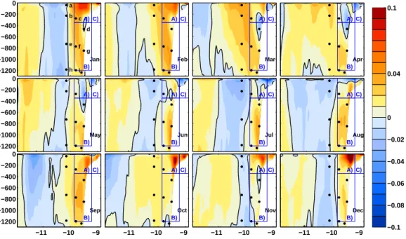
2.2 Seasonal currents 29 −0.1 −0.08 −0.06 −0.04 −0.02 0 0.04 0.1 a b c d e f g h i j Jan A) B) C) −11 −10 −9 −1200 −1000 −800 −600 −400 −200 0 Feb A) B) C) −11 −10 −9 Mar A) B) C) −11 −10 −9 Apr A) B) C) −11 −10 −9 May A) B) C) −11 −10 −9 −1200 −1000 −800 −600 −400 −200 0 Jun A) B) C) −11 −10 −9 Jul A) B) C) −11 −10 −9 Aug A) B) C) −11 −10 −9 Sep A) B) C) −11 −10 −9 −1200 −1000 −800 −600 −400 −200 0 Oct A) B) C) −11 −10 −9 Nov A) B) C) −11 −10 −9 Dec A) B) C) −11 −10 −9
Figure 2.5: Section I (see Fig. 2.1) - Vertical sections of the monthly averages of 20-years simulation of alongshore velocities (m s−1) - positive values correspond
to northward flow. The black dots represent the position of the current meters available for the section (labeled in the January field). The 3 areas represented with blue boxes (A, B, C) are used to compute integrated transport in section 2.2.2.5.
30 2. Seasonal Cycle of the IPC and other Alongshore Flows −0.1 −0.08 −0.06 −0.04 −0.02 0 0.04 0.1 b c d a e f g h i j k l Jan A) B) C) −11 −10 −9 −1200 −1000 −800 −600 −400 −200 0 Feb A) B) C) −11 −10 −9 Mar A) B) C) −11 −10 −9 Apr A) B) C) −11 −10 −9 May A) B) C) −11 −10 −9 −1200 −1000 −800 −600 −400 −200 0 Jun A) B) C) −11 −10 −9 Jul A) B) C) −11 −10 −9 Aug A) B) C) −11 −10 −9 Sep A) B) C) −11 −10 −9 −1200 −1000 −800 −600 −400 −200 0 Oct A) B) C) −11 −10 −9 Nov A) B) C) −11 −10 −9 Dec A) B) C) −11 −10 −9
Figure 2.6: The same as Fig. 2.5, for section II (see location on Fig. 2.1).
−0.1 −0.08 −0.06 −0.04 −0.02 0 0.04 0.1 b c da e g h f Jan A) B) C) −11 −10 −9 −1200 −1000 −800 −600 −400 −200 0 Feb A) B) C) −11 −10 −9 Mar A) B) C) −11 −10 −9 Apr A) B) C) −11 −10 −9 May A) B) C) −11 −10 −9 −1200 −1000 −800 −600 −400 −200 0 Jun A) B) C) −11 −10 −9 Jul A) B) C) −11 −10 −9 Aug A) B) C) −11 −10 −9 Sep A) B) C) −11 −10 −9 −1200 −1000 −800 −600 −400 −200 0 Oct A) B) C) −11 −10 −9 Nov A) B) C) −11 −10 −9 Dec A) B) C) −11 −10 −9
2.2 Seasonal currents 31
2.2.2.4 Comparison with current meter data
Figures 2.8, 2.9 and 2.10 show a comparison between model and current meter time series statistics for the alongshore velocity component. Each subplot corresponds to a current meter location (see black dots in the velocity cross sections of Figures 2.5, 2.6 and 2.7, for section I, II and III, respectively) and the plots are aligned according to the position of the current meters: the left to the right corresponds to the offshore to the coast and top to the bottom corresponds to the depths of the current meters. We computed monthly averages of the current meter alongshore velocity whenever there were a minimum of 14 days of data per month (missing points correspond to values below that threshold). We also computed monthly averages of the model in the locations of the current meters.
In general, for all the 3 sections, the current meter averages lie inside the shaded area. There is a better correspondence between model and data for the time series closer to the coast, as compared to those offshore (see the values of root mean square error RMSe on the plots, as a measure of cor-respondence between model and observations). This makes sense, because there is a stronger signal of the seasonal cycle closer to the coast (as shown in Fig. 2.4). In these areas where seasonal variability is small compared to in-terannual or eddy induced variability, we should not expect a good agreement between the seasonal cycle of the model and that of the observations.
In section I (Fig. 2.8) the match between the model and the observations is reasonable, even offshore, unlike what happens in the other sections. This is because in this section the 6-month period sinusoid explains a significant part of the variability, associated with the offshore propagation of the av-erage cyclonic cells C1 and C2, described in section 2.2.1. Since this signal is observed in the current meter data at the same locations, it provides fur-ther evidence that the offshore propagation of these anomalies is something recurrent and realistic in a seasonal cycle.
Fig. 2.9 shows the comparisons for section II. In the offshore locations (current meters a), g), h), j) and k) - see positions on Fig. 2.6) there is