305
Abstract
In this study, the variance of ordinary sieving test error was determined concern-ing the specification limit of sized iron ore product by subtractconcern-ing the fundamental error (described by the Gy’s formalism for sampling), from the global error (recover-able from database of historical values). The results allowed the calculation of the confidence interval for the percentage of material finer than the upper screen specifica-tion limit. Thereafter, a method to estimate the so-called effectiveness coefficient of the screening operation was developed, which is the ratio between number of particle presentations to passage and the number of oscillations during the material shaking on the screen surface. This estimation was based on the probability statements and particle size distribution of the feed. Considering the size distribution of the products tested in this study, the results have shown that the sieving time could be reduced when determining the percentage of material finer than the upper specification mesh.
Keywords: screening, sampling theory, Gy's formalism, iron ore.
Tulio Viegas Bicalho Resende
Engenheiro Químico, M. Sc. em Engenharia Mineral Faculdade Pitágoras
Curso de Engenharia de Minas Belo Horizonte - Minas Gerais – Brasil [email protected]
José Aurélio Medeiros da Luz
http://orcid.org/0000-0002-7952-2439 Professor Associado
Universidade Federal de Ouro Preto – UFOP Escola de Minas
Departamento de Engenharia de Minas Ouro Preto - Minas Gerais - Brasil [email protected]
Error variance of
short duration sieving
Mining
Mineração
http://dx.doi.org/10.1590/0370-44672015710008
1. Introduction
A check routine for the accuracy and precision of the methods used in the selec-tion, preparation and testing of particu-lates is required to ensure representative samples for an industrial quality control. The sieving process is distinguished by an easier detection of sampling bias (Gy, 1992). This feature makes it a checker for sampling accuracy, since the sieving
standard procedure could be controlled and the sieving test error is known from a plant history basis.
Grigorieff et al. (2004) studied the influence of the preparation protocols on the global estimation error. The authors compared some preparation protocols by measuring the ash content of pairs of coal samples obtained from the splitting
of global samples. By this method, the difference in chemical analysis (statisti-cal deviation) was approximated to the accuracy of the global estimation error. Considering that for sieving there is no comminution, the technique could be adapted for estimating the variance of the sieving test error and guarantee its role in ensuring sampling quality.
A batch L is homogeneous when the proportion of a component of interest aL
is distributed according to a perfect uni-form distribution. It means that for every
component aU, the following relationship
au=aL is met.
If the batch consists of a total mass ML, NF fragments with an average mass Mi =ML/NF
and the content of the critical component is
aL, then the contribution of each individual fragment i to heterogeneity hi is expressed by the following equation (Pitard, 1993):
2. Literature review
This definition takes into account the mass of the fragments; therefore those
that are heavier have more influence on heterogeneity than the lighter ones. The
constitutional heterogeneity is defined as the variance of hi (Pitard, 1993):
where i =1,2,3…NF.
The formula for the constitu-tional heterogeneity applies only to an isolated finite population of units
Uu. It means that the calculation requires the knowledge of the total number of fragments in the batch never determined in practice. As an
approximation, we use the constant factor of constitution heterogeneity,
HIL, which is independent of the lot size (Pitard, 1993):
(1)
306
The constant “factor of constitution heterogeneity, HILof a particular size class
of interest is calculated by the following approximation (Gy, 1992):
(3)
(4)
Where: MCis the mass of the average fragment of the size class whose invariant heterogeneity is to be estimated;
ac is the proportion of the size class of interest;
k is the representation of each size class of the average fragment that characterizes the particle size distribution of the product;
Fk is the average fragment of each size class k;
Mk is the mass of the average frag-ment of each size class k;
ak is the proportion of each size class. In addition, the following equa-tions hold:
(5)
(6)
(7)
(8)
(9)
(10)
(11) Where, f is the dimensionless shape factor,
accepted around 0.5 (for this material); ρ is the average true density of the material [kg/m³];
dC is the average particle size of the size class whose invariant heterogeneity is
to be estimated;
dk is the average particle size of each size class k.
The fundamental sampling error FSE is defined as the one that occurs when the perfect sampling requirements
are met; it is generated only by the con-stitutional heterogeneity (Gy, 2004). Considering a uniform probability P of selecting the fragments, the variance of the fundamental sampling error can be expressed as:
If the selecting probability P is valid for an individual particle, the
rela-tionship Ms=PML is met, and this implies the following relationship:
Where Ms is the sample mass or an in-termediate portion selected at any step of a sampling protocol and ML is the lot mass or that one of an immediately
preceding step in which the mass MS
was extracted.
From the replacement of invari-ant heterogeneity for a particular size
class of interest at the definition of the variance of the fundamental sam-pling error, the following relationship is met:
According to Gy (1992), the rela-tive difference between the critical content, as, of the sample and that one of the sampled lot, aL, is represented
by the relative sampling error (TSE). Whilst the relative difference between the analytical result aR and the content
aL is denoted by the total analytical
er-ror (TAE). The global estimation error is met when considering those errors as stochastically independent:
Process variability
The overall variability of an indus-trial process comprises the instantaneous
variability and that one resulting from the quality shifts over time. Under these
aspects, the overall variation of a process is represented by:
The first term of the last equation is obtained by taking samples within subgroups with the interval between them close to zero. The second
varia-tion term is obtained by measuring the dispersion between the subgroups.
Then, the variance within the subgroups can be estimated from
307 Where the constant d2 is tabulated for
various sample sizes (for subgroup of size two, 1/d2 = 0.886).
According to the method used by
Grigorieff et al. (2004), the global esti-mation error can be approximated by sampling ranges, since only Gaussian stochastic variability occurs. From the
replacement of the global estimation er-ror by the within subgroup variance, the overall analysis error is determined by the following:
(12)
(13)
(14)
(15)
(16) As an additional remark, it is
note-worthy that although it is widely used, Gy's formalism is based on generalized indices (and therefore approximate),
not explicitly taking into account the actual features of the material under analysis. To tackle this drawback, the use of protocols that lead to the
calibration of the system under study is recommended. An example, applied to samples of bauxite, is developed by Bortoleto et al. (2014).
Likelihood of passage in screening
The probability of a fragment of size d passing through a mesh sieve of aperture a is always less than unity, as the lower the relationship (a - d), the lower that probability is (Gy, 1992). However there are fragments, ap-proximate to the nominal size of the
aperture size d ≈ a, that can both be retained or pass through the screen. At a hypothetical experiment in which the assay material was repeatedly sieved, the same fragments could be either retained or passed through the mesh, since the probability of passage at
exactly the same point is infinitesimal. The probability of an isolated spherical particle, with a single and orthogonal presentation, passing through the surface of an opening square screen was established by Gaudin (1975):
Where j is the wire thickness, a is the mesh aperture and d is the particle
di-ameter.
The probability pn of passage for n
is calculated by the following equation:
Where p1 is the probability of pass-i n g t h r o u g h t h e s c r e e n w pass-i t h a single presentation.
The number of presentations (n) over the screen is a function of crowding and resi-dence time, τ, considering an effectiveness y
of the operating frequency f (according to an approach developed by Carvalho & Luz, 2005), as provided in the following equation:
Law of total probability
Considering A1,A2… An as mutually exclusive events and P( B|An ) an arbitrary
event of the conditional probability of B
assuming An then:
3. Methods
308
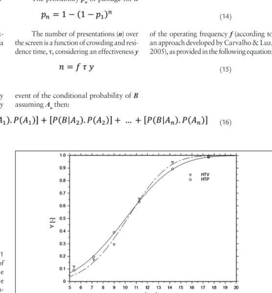
Two products processed at two typical iron ore processing plants, between September 2012 and September 2013, were sampled to have the error variance of their oversize fraction assayed in a sieving test. The sieve chosen was that concerning a 19.0 mm aperture, which is the upper specification limit and that one for which
the whole mass assayed had contact. It is observed in Figure 1 that the two products studied, named HTP and HTV, have a similar particle size distribution. More-over these are also products whose quality remained stable during the increment col-lection period, meaning that the Pearson’s coefficient of variation in production was
about 10 % for the measurement of that retained in the 19.0 mm screen.
There are high correlation coeffi-cients for Rosin-Rammler-Sperling-Ben-nett distributions which are displayed in Figure 1 and is expressed by the following equation:
(17)
(18) In turn, Table 1 presents the size
distribution parameter of those
corre-sponding equations for the two products (obtained by EasyPlot software package).
Product Median diameter (x50) [mm] Sharpness index (m) [-] Coefficient of correlation[-]
HTP 12.804 4.1127 0.9915
HTV 12.6148 3.4035 0.9988
Table 1
Distribution parameter of Rosin-Rammler-Sperling-Bennett distributions for the samples
Linear samplers, which were set according to the parameters listed in Table 2, were used for the selection of forty global samples of 120 kg. These were dried in thermal plates at a maximum temperature of
160 °C and split into samples i and ii, as shown in Figure 2. After that, mass reduction was determined to obtain the required amount so that the same variance of the fundamental sampling error was achieved. For the sampling
preparation protocol, each change in mass was individually considered; therefore, the variance of the funda-mental sampling error was obtained by summing the variance error at each step, as the following:
As shown in Table 3, the HTV’s samples were first split into aliquots of 60 kg and then into the assay por-tions of 20 kg, whereas the HTP’s samples were divided from 60 kg into 18 kg. After many prospective tests, in order to adjust the duration of the
sieving operation, the effective experi-mental campaign was held at a square (500 mm x 500 mm) automatic sieve with timer set to 5 minutes and shaking frequency of 20 Hz, which means 6,000 vibrations. The screens frames (with 100 mm in height) were mounted in
ascend-ing order of openascend-ing 6.3 mm, 8.0 mm, 10.0 mm, 12.5 mm, 16.0 mm and 19.0 mm. The experiments were carried out, registering the proportions of material retained at the 19.0 mm screen for sam-ples i and ii, according to the flowchart of Figure 2.
Product Number of Increments Incremental mass [kg] mass [kg]Sampling [ton/h]Q Sampler slots [m]
Sampler cutting velocity v
[m/s]
HTP 15 7.99 120 230.0 0.075 0.6
HTV 14 8.68 120 250.0 0.075 0.6
Table 2
Samplers parameters obtained according ISO 3082.
Product HIL [kg] mass [kg]Batch MS1[kg] MS2[kg] σ2 (FSE)1 σ2 (FSE)2 σ2(FSE)
HTP 0.632 120 60 18 5.27E-03 2.46E-02 3.0E-02
HTV 0.708 120 60 20 5.90E-03 2.36E-02 2.9E-02
Table 3
Required mass for an
equal fundamental sampling error.
Figure 2
309 From the average range of the results
of samples identified in the diagram of Figure 2 by i and ii, the variance of the global estimation error (0,886 x R )2 a
L
-2was
determined. The variance of the sieving
test error of that retained in the 19.0 mm screen was calculated by subtraction of the variances of the global estimation error and the fundamental sampling error. The average percentage of material finer than
19.0 mm was determined by the difference between 100 % and the average percentage retained by the 19 mm screen. The confi-dence interval was calculated considering that the error follows normal distribution:
The passage probability through the 19.0 mm screen to the HTP and HTV was estimated by calculating the minimum number of presentations required for the sieving test. As such, the following ap-proximations were done:
• the probability of passage through the 19.0 mm screen was considered as
be-ing that determined by Gaudin's equation; • t h e p r o b a b i l i t y o f f i n d -ing any particle size in the product was considered equal to the average size distribution.
From both considerations, by mul-tiplying the passage probability of each fragment size through the 19 mm screen
with the average retained percentage of the size class, and using the law of total probability, the probability of all classes pass through the upper specifica-tion screen was added to the results. In summary, the percentage of passing the 19.0 mm screen was determined with the following the equation:
(19)
Where k corresponds to any size class. The number of presentations n
that is needed for obtaining a
propor-tion corresponding to that of the lower limit of the confidence interval was de-termined from an iterative calculation
method using the goal seek function in Excel.
(20)
4. Results and discussion
The relative error variances are presented at Table 4. As the calculated
values are close to each other, there is a standardized experimental condition for
both products.
Products s2 (GEE) s2 (TAE) s2 (GEE)
HTV 0.066 0.036 0.066
HTP 0.056 0.026 0.056
Table 4 Relative Error Variances.
The lower limit of the confidence interval for the percentage of material finer than 19.0 mm was determined from the variance of the sieving test error shown in Table 4. Using an
iterative method of calculation, the number of presentations needed for the percentage of materials finer than 19.0 mm equal to those of the lower limit of the confidence interval was
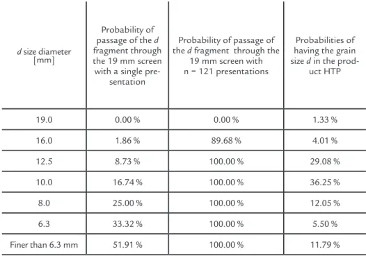
identified. The results were up to 153 presentations for HTV to the sieve mesh (wire thickness: 3.0 mm) and up to 121 presentations for HTP, as presented in Tables 5 and 6.
d size diameter [mm]
Probability of passage of the d fragment through the 19 mm screen with a single
pre-sentation
Probability of passage of the d fragment through the
19 mm screen with n = 121 presentations
Probabilities of having the grain size d in the
prod-uct HTP
19.0 0.00 % 0.00 % 1.33 %
16.0 1.86 % 89.68 % 4.01 %
12.5 8.73 % 100.00 % 29.08 %
10.0 16.74 % 100.00 % 36.25 %
8.0 25.00 % 100.00 % 12.05 %
6.3 33.32 % 100.00 % 5.50 %
Finer than 6.3 mm 51.91 % 100.00 % 11.79 %
Percentage of particles finer than 19 mm: 98.25 % Table 5
310
d size diameter [mm]
Probability of pas-sage of the d fragment
through the 19 mm screen with a single
presentation
Probability of passage of the d fragment through the 19 mm screen with n = 153
presentations
Probabilities of having the grain size d in the
prod-uct HTV
19.0 0.00 % 0.00 % 1.48 %
16.0 1.86 % 94.34 % 9.29 %
12.5 8.73 % 100.00 % 26.02 %
10.0 16.74 % 100.00 % 24.28 %
8.0 25.00 % 100.00 % 19.30 %
6.3 33.32 % 100.00 % 10.65 %
Finer than 6.3
mm. 51.91 % 100.00 % 8.98 %
Percentage of particles finer than 19 mm: 97.97 %
Table 6
Estimation of the number
of presentations for the product HTV.
Although there are more finer par-ticles at HTP in comparison to HTV, its size distribution where there is a larger quantity of fine fragments with a higher probability of passing through the 19 mm testing screen in comparison to the HTV, implies in less presentations required overall.
The effectiveness of the operating frequency (y) to obtain the lower limit of the confidence interval was approxi-mately 0.02. This result indicates a great deviation from the optimum condition for effectiveness, y = 1, wherein the par-ticle presents itself isolated for screen-ing. This indicates that the assay was
conducted with the testing screen full of retained material or that the procedure time was longer than was really needed. As there is a low percentage of particles in the two products that are larger than 19.0 mm, about 1 %, the passage of all fragments over that screen occurs in a much shorter time than 5 minutes. If only the information about 19 mm screen was needed, the proper thing to be done would be a reduction of the time assay to 6 seconds.
As far as the sieving time is con-cerned, it is important to note that, although 5 minutes would definitely not be enough time for good sieving
efficiency in a conventional sieve test, in the present case, a majority of the fractions are clearly coarse classes (between 6 and 19 mm) as well as the control mesh (19 mm).
On the other hand, some re-marks on the amount of particulate material for sieving are also ap-propriate. After linear regression of data from the Washington State Department of Transportation (2017) on sieve analysis of aggregates, one can express the maximum mass (in kg) per square meter of sieve sur-face (with correlation coefficient
R2 = 0.999998) according to:
(21)
Where A is the effective sieving area (in square meters) and x is the mesh aperture (in meter). Note that, for x = 19.0 mm and A = 0.25 m² the maximum allow-able charge would be: mmax = 11.88 kg.
However, it should be borne in mind that coarse aggregate's bulk density (typically 1.7) falls below that of iron ore concen-trates (typically 2.7). Using the ratio of such figures of density as the scaling
factor, it results in a maximum of about 19.0 kg. Thus, also under this criterion, the volumetric limit has not been ex-ceeded after all, keeping the validity of the conclusions herein.
5. Conclusion
The technique adapted for estimat-ing the variance of the sievestimat-ing test error has shown the standardized condition for characterization of the tested products. Therefore, this could be a useful tool to ensure good sample quality.
The method developed to identify the effectiveness of operating frequency
y for the sieving test has shown that the usual sieving operation is largely within the range of safety, since the minimum duration value calculated is smaller than that practiced in routine tests for the bulk material under study. The Authors think that continuity of this study is appropri-ate to extend the analysis of the sieving
311
References
BORTOLETO, Daniel Armelim et al. The application of sampling theory in bauxi-te protocols. Rem: Rev. Esc. Minas, Ouro Preto, v. 67, n. 2, p. 215-220, June 2014. Available from <http://www.scielo.br/scielo.php?script=sci_arttext&pid =S0370-44672014000200014 &lng=en&nrm=iso>. Access on 26 Feb. 2018. http://dx.doi.org/10.1590/S0370-44672014000200014.
CARVALHO, Simão Célio de; LUZ, José Aurélio Medeiros da. Modelamento ma-temático de peneiramento vibratório (Parte 2): simulação. Rem: Rev. Esc. Minas, Ouro Preto , v. 58, n. 2, p. 121-125, June 2005. Available from <http://www. scielo.br/scielo.php?script= sci_arttext& pid=S0370-44672005000200005& lng=en&nrm=iso>. Access on 26 Feb. 2018. http://dx.doi.org/10.1590/S0370-44672005000200005.
GAUDIN, A. M. Principles of Mineral Dressing. 1st ed. New York: McGraw-Hill Book Company, 1939. 554 p.
GRIGORIEFF, A.; COSTA, J. F.; KOPPE, J. Quantifying the influence of grain top size and mass on a sample preparation protocol. Chemometrics and Intelligent Laboratory Systems, Amsterdam, v. 74, n.1, p. 201-207, 2004.
GY, P. M. Sampling of Particulate Material: Theory and Practice. 1st ed. Amsterdam: Elsevier, 1979. 43 p.
GY, P. M. Sampling of Heterogeneous and Dynamic Material Systems: 1st ed. The-ories of Heterogeneity, Sampling and Homogenizing. Amsterdam: Elsevier, 1992. 652 p.
GY, P. M. Sampling of discrete materials: a new introduction to the theory of sampling I. Chemometrics and Intelligent Laboratory Systems, Amsterdam, v. 74, p. 7–24, 2004.
ISO. 3082. Iron ores — Sampling and sample preparation procedures. Geneva: ISO, 2017. 83 p.
MINKKINEN, P. Practical applications of sampling theory. Chemometrics and Intelligent Laboratory Systems. Amsterdam, v. 74, n.1, p. 85–94, 2004.
MOGENSEN, F. A New Screening Method of Screening Granular Materials. The Quarry Managers’ Journal, p. 409–414. Oct., 1965.
MONTGOMERY, D.C.; RUNGER, G.C. Applied Statistics and Probability for Engineers. 5th edition. Phoenix: John Wiley & Sons, 2011. 768 p.
PITARD, F. F. Pierre Gy's Sampling Theory and Sampling Practice. 2nd edition. New York: CRC Press, 1993. 488 p.
WASHINGTON STATE DEPARTMENT OF TRANSPORTATION. Sieve Analysis of Fine and Coarse Aggregates. In: WASHINGTON STATE DEPART-MENT OF TRANSPORTATION (Ed.). Materials Manual M 46-01.27 T 11. Olympia: WSDOT, 2017. p. 1–14.