Essays on Bounded Rationality: Individual Decision and Strategic Interaction

(1)

Nova School of Business and Economics Universidade Nova de Lisboa

Thesis, presented as part of the requirements for the Degree of Doctor of Philosophy in Economics

Essays on Bounded Rationality: Individual Decision and

Strategic Interaction

Pedro Maria Bonneville Chaves 566

June 30, 2015

(2)

Abstract

Economics is a social science which, therefore, focuses on people and on the decisions they make, be it in an individual context, or in group situations. It studies human choices, in face of needs to be fulfilled, and a limited amount of resources to fulfill them. For a long time, there was a convergence between the normative and positive views of human behavior, in that the ideal and predicted decisions of agents in economic models were entangled in one single concept. That is, it was assumed that the best that could be done in each situation was exactly the choice that would prevail. Or, at least, that the facts that economics needed to explain could be understood in the light of models in which individual agents act as if they are able to make ideal decisions. However, in the last decades, the complexity of the environment in which economic decisions are made and the limits on the ability of agents to deal with it have been recognized, and incorporated into models of decision making in what came to be known as the bounded rationality paradigm. This was triggered by the incapacity of the unboundedly rationality paradigm to explain observed phenomena and behavior. This thesis contributes to the literature in three different ways.

Chapter 1is a survey on bounded rationality, which gathers and organizes the contributions to the field sinceSimon(1955) first recognized the necessity to account for the limits on human rationality. The focus of the survey is on theoretical work rather than the experimental literature which presents evidence of actual behavior that differs from what classic rationality predicts. The general framework is as follows. Given a set of exogenous variables, the economic agent needs to choose an element from the choice set that is avail-able to him, in order to optimize the expected value of an objective function (assuming his preferences are representable by such a function). If this prob-lem is too complex for the agent to deal with, one or more of its eprob-lements is simplified. Each bounded rationality theory is categorized according to the most relevant element it simplifies.

(3)

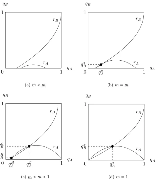
operations. In our model, if they choose not to think, such cost is avoided, but they are left with a single alternative, labeled the default choice. We ex-emplify the idea with a very simple model of consumer choice and identify the concept of isofin curves, i.e., sets of default choices which generate the same utility net of thinking cost. Then, we apply the idea to a linear symmetric Cournot duopoly, in which the default choice can be interpreted as the most natural quantity to be produced in the market. We find that, as the thinking cost increases, the number of firms thinking in equilibrium decreases. More interestingly, for intermediate levels of thinking cost, an equilibrium in which one of the firms chooses the default quantity and the other best responds to it exists, generating asymmetric choices in a symmetric model. Our model is able to explain well-known regularities identified in the Cournot experimental literature, such as the adoption of different strategies by players (Hucket al. , 1999), the inter temporal rigidity of choices (Bosch-Dom`enech & Vriend,

2003) and the dispersion of quantities in the context of difficult decision mak-ing (Bosch-Dom`enech & Vriend,2003).

(4)

leads to low turnout (Geys,2006), a lower margin of victory when turnout is higher (Geys,2006) and high turnout rates favoring the minority (Bernhagen & Marsh,1997).

(5)

(6)

Acknowledgements

I am grateful to Funda¸c˜ao para a Ciˆencia e Tecnologia for a 48 month scholarship, which provided an essential financial support for the completion of this thesis.

Also, I thank Nova School of Business and Economics, for allowing me to work as a teaching assistant. Not only for the financial support, but, most importantly, for giving me the opportunity to teach. All the math that is in the thesis would probably be replaced by conjectures and vague propositions, hoping no one would notice it, if I had not learned everything I did while teaching. Of course, I also have to mention all the assistance to the completion of this thesis directly provided by the school, either by supporting the attendance of conferences, organizing seminars to discuss work in progress, or introducing annual assessments, which always made me feel uncomfortable. And that is exactly what I needed.

Specifically, I have to recognize the contributions from all faculty members with whom I talked about the contents of this thesis. While some times the ideas I presented deserved to get an unpronounceable answer, they were nothing but kind and helped me find the right direction, which I hope to have done. Jo˜ao Furtado deserves a special mentioning here. Not only did he directly contributed to the third chapter of this thesis, by, being smart as usual, creating the concept of rhizomatic thinking, but he was also incredibly available to debate ideas, in discussions that lasted for hours and usually ended up as philosophical arguments. Thank you for all the interest you put in my ideas.

(7)

Behavioral Economics. The first and second chapters of this thesis have an enormous contribution from him. And the football moves he taught me, which I thought were not anatomically possible, were also an inspiration in life.

I am very grateful to all my friends and students for eventually learning that a PhD thesis is like Voldemort. It should be known as the one that shall not be mentioned. I know I did not always reacted in the most pleasant way when you asked about the delivery date, and I am sorry for that, especially because you were only showing that you cared. The good news is that I now have an answer: it is done.

There are some friends which did more than simply ask about this thesis. And they are part of the reason why I now have an answer to all the others. I thought about mentioning them by name, but preferred not to. This way, I can say to anyone who asks: ‘Do you think I would forget you?’

I would like to thank my family members one by one, but, unfortunately, it is a rather big family. So, let me thank all of them for tolerating my ‘occasional’ bad mood. You were all a bigger help than you can imagine. But please do not ask me again to explain what the thesis is about. Just read it.

(8)

Introduction

Economics can be thought of as the study of the decisions and actions of people who have to use the available resources to fulfill their needs. It is exactly this focus on people that makes Economics a social science. And its socialness has advantages and disadvantages. On the plus side, it is not a closed science, centered on itself, but can be used to observe, analyze and predict real phenomena, events and actions, and therefore to better understand the world we live in. However, its human centering prevents it from having hypotheses as testable and predictions as accurate as some natural sciences. In fact, human activity is ruled by human decisions and these are the result of each person’s brain functioning. And here, scientists face two major problems. First, in spite of the advances in neurology and neuroeconomics, we are still unable to analyze the exact way decisions are made and, therefore, cannot predict with certainty what every individual will do in every situation. Second, even if we could do that for a specific person, we would still be far from being able to explain most social phenomena, as it seems that different people act differently in similar contexts.

(11)

gathering of everyone’s decisions cancels individuals mistakes and the aggregate result is somewhat close to the optimum. In these cases, the assumption of individual unbounded rationality does not harm the validity of the collective result. And in other situations, although people do not optimize the problem they face, they end up choosing the optimal action, either by randomizing, or by using another decision process which coincidentally results in selecting the optimum. However, it seems unreasonable to assume that unbounded rationality is used by all agents in all situations. There are some situations in which the optimal decision is so hard to find for the modeler (who can take the time and use the auxiliary resources needed to formalize the problem, find how to solve it, and execute calculations), that it seems implausible that an individual, when faced with the problem, having to make a decision on a short period of time, and relying on nothing but himself, is able to find the optimal solution by other than chance.

Even if one is happy with the results obtained from the use of unbounded ratio-nality, the concern with this kind of issues seems important at least from a procedural point of view. When you first contact with Economics, you learn that models are a simplified version of reality, which allows you to study it in a tractable way and to get predictions which otherwise would be impossible to get. Then, one of the most important tasks faced by a modeler is to choose which aspects of reality should be simplified or ignored, and which ones should be kept unchanged. It is understand-able that, in Economics, rationality is normally chosen as one aspect to be simplified, if nothing else, because we don’t understand entirely how it works. However, being human decisions as important as they are in economic models, the level of sim-plification that unbounded rationality implies makes some authors believe that it should be replaced by some other concept closer to the way in which people actually think. Even if this does not the improve the quality of the results obtained, the movement in this direction is at least an honest attempt to make economic models more realistic regarding one of its core features: decision processes.

(12)

stated, the task is to replace the global rationality of economic man with a kind of rational behavior that is compatible with the access to information and the com-putational capacities that are actually possessed by organisms, including man, in the kinds of environments in which such organisms exist.” Since then, many au-thors acknowledged the existence of this problem and have proposed some solutions. However, bounded rationality is very difficult to model in an unified way, because this would imply the knowledge of all determinants of human behavior, which we are still far from getting. Indeed, the most difficult object of investigation for man seems to be man himself. And this partly explains why bounded rationality has spread in so many different directions.

This diversity motivated Chapter 1. It is a survey on bounded rationality, cov-ering contributions to the field from Herbert Simon’s pionecov-ering work in satisficing

(Simon,1955) to recent developments, such as the notion ofsparsity (Gabaix,2014). To select what literature we should analyze, we had to define a criterion. Especially because bounded rationality is part of a wider field, Behavioral Economics. This recent field in economic history gathers contributions from different sciences, such as psychology, sociology and neuroscience, to construct a view of human behavior that accounts for the factors that influence the human mind. However, Behav-ioral Economics does not necessarily assume that rationality is bounded. In fact, concepts like reciprocity, fairness or loss aversion do not imply that people find it difficult to solve any specific problem. Instead, their human nature influences their decisions, because they care about certain aspects that traditional Economics failed to acknowledge, or decided to ignore. The perspective we take here is that bounded rationality takes its place whenever the contrast between the complexity of the decisional environment and people’s abilities to solve problems affect the way in which such problems are viewed or dealt with. That is, we only focus on problems which are simplified or transformed in such a way that they become easier to analyze according to people’s views on them.

(13)

simplified, then we should be able to identify what is changed relatively to the classic perspective. But, if we are to do this, we need to have in mind what constitutes any economic problem. This led us to the recognition of six elements. If a choice has to be made, one or more alternatives must be available. This means a choice set, the first element, must be defined. Then, some kind of ranking of elements of the choice set must exist, because otherwise no decision was needed. Thus, preferences of the decision maker should be specified and, if possible, represented by an objective function, the second element. If, indeed such function exists, and its optimization is difficult, we need to specify how an agent tries to reach the best decision possible. That is, the third element, an optimizer operator, defines the procedure used to make a choice. And, technically, a decision maker needs to understand what, in the problem at hand, requires a decision. This generates the set of decision variables, the fifth element. Finally, the problem, specifically the objective function and the choice set, may be influenced by factors out of control of the decision maker. These external elements, parameters, are the fifth element we analyze. Finally, the decision maker may not possess all the information that affects the problem, but still need to make a decision. This is the basis for the sixth element, the uncertainty operator. Notice that models of strategic interaction between different players, may, in general, be accommodated in this framework, because each player is solving his own problem, and does not control other players’ decisions. However, given the specificity of such models and the importance they have in economic modeling, we cover them separately. After the review of the literature in bounded rationality, we make two contributions to the field, one affecting individual decision and the other specifically designed for strategic interaction contexts. They are presented in Chapter 2 and Chapter 3, respectively.

(14)

suggestion from other people (Choiet al. ,2003), the optimal choice associated with a standard, although not necessarily true, view of the world (Gabaix, 2014) or in other ways. What is important about it is that it provides the agent an alternative to thinking. A costly thinker then has to decide, besides an option from the original choice, whether to think on the problem, or to stick to his default choice. If he does decide to think, the cost of doing so is subtracted to the payoff he gets, and this frames thinking as any other scarce resource resource in economic problems. Its benefit and cost must be compared, in order before a decision about its use is made. Before moving to the main application of the concept, we apply it to a very simple consumer problem, for illustrative reasons. Interpreting the default choice as the result of intuition, we conclude that consumers with a good intuition decide not to think, because the benefit in finding the optimal choices is outweighed by the cost it implies. And to have a good intuition, in this context, means to have a default bundle that the consumer highly values. On the other hand, consumers who find it more difficult to think rely more on their intuition.

(15)

Vriend, 2003). Strategy heterogeneity is obtained endogenously when the thinking

decision is different between firms. Inter temporal rigidity, that is, repetition of choices across periods is a result from a dynamic extension of our model, which predicts that, if the thinking cost decreases over time at all but one specific rate, there are some periods in which quantities do not change and, moreover, the firms eventually learn to play the Nash equilibrium and do it forever without thinking. And an increase in quantity dispersion when decisions are harder to make is also a consequence of our model, if we allow for different default quantities and it is obtained in a more pronounced way if more than two firms are considered.

Chapter 3 was written in co-authorship with Susana Peralta. Contrary to the model in Chapter 2, in which the concept we introduced has a direct impact on individual decisions (although it also indirectly influences the outcome of game-theoretical models with players that are boundedly rational in the way we define), in this chapter, we directly approach strategic interaction between players. Based on the notion ofrhizomatic thinking (Bravo-Furtado & Cˆorte-Real,2009a), we say that a player is self-delusional if, when deciding, believes that a fraction of like-minded players necessarily take the same action as he does. This means that self-deluded players believe their decisions have a higher impact on the game outcome than they really have, because the players they assume to act as they do, may, in fact behave differently. This type of belief simplifies the game, because the number of players whose strategies need to be forecast is reduced. A natural application for this concept is the problem of voter turnout. Indeed, in large elections, the small expected impact of each single vote combined with a positive cost of voting, even if very low, results in the theoretical prediction of no voting, which is clearly contradicted by reality. The empowerment that self-delusion provides to potential voters may then explain why it is that they actually vote.

(16)

(17)

(18)

Chapter 1 The Simplified Economic Problem:

A Survey on Bounded Rationality

1.1 Introduction

Behavioral Economics is a relatively recent field. Its creation was a response to concerns about the assumptions on human behavior in economic models, as were made until then, and their impact on the quality of predictions. Contrary to the predominant practice at the time, this field had a clear focus on the connection between human reasoning and observed decisions. It proposed to reach to other sciences, such as psychology, sociology and human science, in order to better un-derstand the way in which people actually think, and construct more realistic and successful models of human behavior. This movement made possible the appear-ing of novel theories such as hyperbolic discounting (Laibson,1997), prospect theory

(Kahneman & Tversky, 1979), fairness and reciprocity (Rabin, 1993) and altruism

(19)

a different perspective. They consider that some problems are too hard to be solved by agents with bounds on their reasoning abilities. It is not just a matter of how limited an agent is, but, more generally, of what results from the contrast between his difficulties in thinking and the complexity of the decision he faces. And this idea is the core of bounded rationality.

The contributions to the literature on this theme have been the object of some surveys. March (1978) centers his analysis on the problem of choice and discusses how it is affected by bounded rationality and changes in the way preferences are modeled. Camerer (1998) mainly focuses on experiments that either motivate the creation of theoretical models, or test them. Conlisk (1996b) presents evidence of bounded rationality, shows the success of some papers in this area, discusses the objections against it and defends that it is a part of Economics on its own right, as it deals with the use of a scarce resource, reasoning. Lipman(1995) reviews papers which treat bounded rationality as an information processing problem.

We also review the literature on bounded rationality, but do it guided by a specific view of the concept and how it impacts economic modeling. In Economics, a problem arises when there is the need to allocate limited resources to achieve some goal. That is, whenever there is the need to make a choice between different options. Formally, we think of a general economic problem as:

OptxE♣u♣α, xqqs. t. xPS♣αq (1.1)

There are six elements we identify in (1.1). They are the following:

1. Opt: The optimizer operator. Represents the procedure that is followed to achieve the intended goal. May or may not result in the choice of the best available option.

(20)

3. E: The uncertainty operator. An agent may not possess all the information he needs to solve the problem, but still need to make a decision. In this case, he must adopt a procedure to deal with the uncertainty he faces, represented by this operator.

4. S: The choice set. Includes the options the agent considers. May be endoge-nous, if the agent has the possibility to filter the options to choose from. 5. α. The parameter set. Consists of all factors that influence the problem, over

which the agent has no control. Includes other players’ decisions in traditional game theory.

6. x: The set of decision variables. Expresses what the agent can control and needs to decide upon.

A bounded rationality model should then simplify an economic problem, in at least one of these elements. We classify what we consider to be the main papers on this theme according to the simplified element that is more relevant in their analysis. Game-theoretic models, given their specificity, are analyzed in their own section, although it would be possible to fit them in one of the six categories, as individual decisions need to be done even in contexts of strategic interaction. Our focus is on theoretical contributions, not on experimental evidence that motivates them. Of course, this is not an exhaustive analysis of the literature on this theme, but a presentation of the papers we feel to be more representative of the advances in this area.

(21)

1.2 Individual Choice

In this section, we present the main theoretical papers which change the classic problem of individual decision. InSection 1.2.1, we focus on the optimizer operator. Changes to the objective function are studied in Section 1.2.2, if they are mere simplifications, and in Section 1.2.3, if they consist on the adding of a thinking cost. The other elements of the economic problem, uncertainty operator, choice set, parameters and decision variables are analyzed inSection 1.2.4.

1.2.1 How to choose

We start with models that assume that people, when confronted with a choice problem, do not try to select the best option available. In the papers we ana-lyze, people search the choice set until finding a satisfactory option (Simon, 1955, Gigerenzer & Goldstein, 1996), adjust their choices over time towards the ones that

are revealed to be more successful (Arthur, 1991, 1994) and allocate their mental resources according to not necessarily optimal rules (Radner & Rothschild, 1975).

One possible method of making choices which are not necessarily optimal is to define what a good payoff would be and try to achieve it. That is, instead of taking the best option from a choice set, take the first one which implies a minimum utility level. This is the basis for the concept ofsatisficing, labeled this way by the formal launcher of the concept inSimon(1956). In a previous paper (Simon, 1955), he developed a framework that allows to adapt a general optimization problem to this concept. In a particular way, Gigerenzer & Goldstein (1996) also employs the satisficing idea. He assumes that, when comparing choices, people look at the characteristics of each of them. Sequentially, they try to rank these characteristics, and stop when they believe to have found conclusive evidence of what is the best option. This does not necessarily results in an optimal choice but, instead, search is stopped when the agent deciding is comfortable with his option.

(22)

and that the human mind is limited in the way it deals with it, implying that optimization may not be possible in some situations and should be replaced with a different choice mechanism. In this paper, the notion of satisficing, although still not labeled this way, is presented for the first time. A satisficer first defines an

aspiration level, that is, a minimum utility level which he is willing to accept. Then, a sequential search is performed in the choice set, and it stops when an alternative that guarantees at least the aspiration level is found, and this is the alternative selected.

More formally, the author proposes the following choice procedure. There is a general choice set, A, and a subset of it, ˜A, is known by the agent. S is the set of consequences the selection of each element in A may have. The utility each consequence in S brings to the agent is defined by V. The agent may have a more limited information on the relationship between ˜A and S and just know what are the possible consequences of each action he can take (if this is the case, eacha inA

is linked to a subset ofS), or he may be more informed, and be able to specify the probability that each possible consequence of a given action will indeed occur if the action is selected. Within this framework, classic rationality would result in the use, for example, of a maxmin rule or expected utility maximization. The behavioral alternative suggested is the simplification of V, which would map elements in S

(23)

iP t1, ..., n✉, and the agent’s objective is to find an a P A˜ that maps into a subset of S containing only consequences s such that ❅iP t1, ..., n✉, Vi♣sq ➙ki.

The model also allows for dynamic considerations. For instance, aspiration lev-els may vary with time, decreasing if satisfactory solutions are hard to find and increasing otherwise, and the choice in each period may be influenced by the results of the choices taken in the past. A final note to mention that the author refers the possibility of accounting for the cost of making complex decisions, which would generate a new, more general problem which could then be optimally solved. This route, however, is not followed, which is justified by the ignorance of the agent of such costs and its inability to compare the utility of each action and the cost of choosing it. Therefore, it is safe to assume that Simon, in his seminal contribution, was hinting at costly thinking, which was developed years later by Conlisk (1980), for example, as a promising research avenue.

Gigerenzer & Goldstein (1996), in a paper published in a psychology journal, present three heuristics to be used when making inductive inferences. They focus on the problem of making a comparative assessment of a set of alternatives, when such comparison is not easy to make directly. Instead, the agent resorts to some features of the alternative objects, labeled cues, which he thinks are good indicators of which choice he should make. Trying to define fast and efficient heuristics, the authors propose three different evaluation methods which make use of cues, but do not require the knowledge of all of them.

Formally, a choice is to me made in a set of nobjects, A✏ ta1

, ..., an_✉_{. Object}_k

has a value t ak✟, and the agent’s goal is to select the highest value choice. There is the possibility that the agent has never heard of one or more of the objects. The recognition of object k by the agent is defined by the binary variable rk P t0,1✉, where 0 stands for ignorance and 1 for recognition. There is a set of m binary cues, which can take the value ✁1 or 1, where the former represents a negative and the latter a positive signal. Cue i, for object k, assumes the value ck

i P t✁1,1✉.

When investigating cki, the agent can either believe it to be 1 or ✁1 or do not

assume anything about it. The agent’s belief about ck

(24)

✁ and ? represent, respectively, the ideas that cki is 1, ✁1 and unknown. If the

agent does not recognize one object, he assumes all its cues to be unknown, i.e., ❅ kP t1, ..., n✉:rk ✏0✟,❅i P t1, ..., m✉, bki ✏?. Cue i has an ecological validity,

represented by vi, which measures its ability in correctly comparing the values of

objects. Specifically, it is the fraction of times that an object has a higher value than another, whenever the cue is positive for the best object and negative for the other. That is:

vi ✏

#✥♣k, lq P t1, ..., n✉2 :cik ✏1❫cli ✏ ✁1❫t ak

✟

→t al✟✭

#✥♣k, lq P t1, ..., n✉2 :ck

i ✏1❫cli ✏ ✁1

✭

The first heuristic proposed by the authors is the Take the Best Algorithm. The agent selects two objects, ak _and _al_{, to compare. If he recognizes only one of them,}

that is the one he chooses. If he recognizes neither, he randomly selects one. If both objects are recognized, the agent ranks the cues by their ecological validity. He sequentially compares his beliefs about the cues, starting with the one with the highest economic validity. If, for cue i, his beliefs are bk

i ✏ and bli ✘ , object k

is selected. Otherwise, the agent moves to the next cue. If this process leads to no objection selection, a random choice is made. If there are no random choices made, this heuristic is transitive, and, independently of the ordering of objects’ pairing, the resulting choice is always the same. The Take the Last Algorithm differs from this in that cues are ordered not by their ecological validity, but rather by their order of use. That is, when comparing two objects, the first cue to be analyzed is the one that settled the last comparison of objects the agent made. In the Minimalist Algorithm, the use of cues is randomly ordered. Notice that, while the Take the Best Algorithm demands the knowledge of ecological validities and the Take the Last Algorithm the memory of discriminating cues, the Minimalist Algorithm needs no information about cues. And they all have in common the use of a subset of cues, which can be very small.

(25)

their population. There were 9 cues used, such as the property of being a national capital or the existence of a local university. The percentage of cities recognized, as well as the percentage of cues known (they assumed that agents either knew the true value of the cue or assumed it to be unknown) varied through simulations. They conclude that, predictably, the heuristic algorithms are faster, in the sense that the number of cues they use is smaller and, to some surprise, that the Take the Best algorithm was the one that had a higher inference accuracy, on average. One curious phenomenon resulted from simulations. For the heuristic algorithms, accuracy was maximized when only some of the objects were recognized. The reason is that the simulations were setup with the property that, with an 80% probability, a recognized object had a higher value than an unrecognized one. Thus, an exces-sive number of recognized objects led to a small number of contests decided by the recognition variable, wasting a quite accurate criteria.

Another not necessarily optimal method of choice is sampling and adjustment, that is, finding the merits of each available option by trying it out. A bounded rational agent that is unable to instantly find an optimum may nonetheless be able to observe the results of his choices, choosing more often the options which perform better through time. This is the basis idea of two papers of the same author,Arthur (1991) and Arthur (1994). An important distinction between them is the object of the agents’ observations. In Arthur (1991), the agent is undecided about what element from a choice set he should take, whereas in Arthur (1994) his indecision is relative to selection rules, that is, criteria he can use to make a choice. Besides, inArthur (1991), there is a mechanism of self-reinforcement, as the selection of an action in one period increases the probability of its selection in the future, but in Arthur (1994), the probability that a selection rule is chosen is not influenced by the fact that it was used in the past, as the agent always looks at all the rules at all times, giving them all an equal opportunity.

(26)

agent has a prior belief about the payoff quality of each action and selects an action using a randomizing profile that takes this belief into account. After an action is randomly selected in this fashion, its realized payoff is registered and the belief is updated, leading to a new random choice.

Specifically, there are N actions, indexed by i. Action i’s payoff is positive and distributed according to the stationary distribution Φi_{, with expected value} _φ

i. For

each period t P t0,1, ...✉, St ✏ ♣Stiqi_Pt1,...,N_✉ is a vector of strengths associated with

each action. The sum of actions’ strengths in period t is Ct and, in this period,

the probability that each action is chosen is its relative strength. That is, if pi t is

the probability that action i is chosen in period t ➙ 1, pi t ✏

Si t

Ct. After the action

selection, the vector of strengths is updated. First, the payoff realized by the chosen action is added to its strength. Then, strengths are normalized so that their sum is

Ct 1 ✏ C♣t 1qν. This implies that, if action j is chosen in period t, its realized

payoff at that time is πj_t, and ej _{is the} _j_{th unit vector,} _S t 1 ✏

C♣t 1qν

Ctν _πj t

St πtjej

✟ .1 The stochastic evolution of the probability of choosing each action is shown to be the following:

❅t P t1, ...✉,❅iP t1, ..., N✉, pit 1 ✏p

i t

✄

1 φ

i_✁➦N j✏1 p

j tφj

✟ Ctν ξt Cν t ☛ (1.2)

In(1.2),ξtis a zero mean disturbance. These dynamics are important in

under-standing and confronting the concepts of exploration and exploitation. The former refers to the analysis of the search set, achieved by selecting different actions over time and allowing to find good alternatives, while the latter means the repeated selection of an alternative which has proven to be good enough. Suppose k is the action with the highest expected payoff andlalso has a high payoff, but not as high. The factors that contribute to the exploitation of l, if it is chosen in early periods, or to the exploration of the choice set and subsequent finding ofk are understood by observing (1.2). The expression φi_✁➦N

j✏1 p

j tφj

✟

stands for the difference between

1

The agent is assumed to have an initial belief about the actions’ strengths, which is represented

by the strictly positive vectorS0. As no choice is made in period 0,S1✏_CC

(27)

the expected payoff of action i and the expected payoff the agent gets, given the probabilities he defines in period t, and is positive for sure when i ✏ k and also positive wheni✏l, if l has a high enough expected payoff. Ifk is significantly bet-ter than its albet-ternatives, this expression attains a high positive value, and pk

t tends

to increase, even if k is not selected often in early periods, preventing the agent’s choice from being locked in a different action. On the other hand, if eitherC or ν

are low, the rate of growth ofpl, ifl is chosen with some regularity in early periods,

is high, and this action may always be chosen from a certain point in time, even if it is not the optimal action. Restricting ν to be in r0,1s, the author states that only when ν ✏1 the locking in of action k is guaranteed. The model is then used to calibrate the values of C and ν against some experiments where subjects had to choose between two actions for 100 periods, and the calibrated model replicated quite well the results of the experiments.

Arthur(1994) argues that human reasoning is essentially inductive, in opposition to the deductive thinking classic rationality assumes. Intuition is defined as a set of beliefs, rules and selection methods, which depend on the context in which they are formed, and evolve over time, with the most successful ones being reinforced and the others discarded. Not knowing how to deal with a specific problem, an agent constructs some models of choice which he can cope with, and compares the results of their application to the problem at hand. Over time, the most successful ones become the most often used.

(28)

uses the method that has proven more accurate at the date, in a process that is constantly updated. The author performs a computer simulation to test this theory, defining that each of the 100 agents knows a subset of the whole set of acting rules. He concludes that, on average, 60% of the rules being used led to attendance, and states that it seems natural that this game is attracted to a Nash equilibrium, where each player goes to the bar with a probability of 60%.

Radner & Rothschild(1975) has in common with Arthur (1994) the fact that it uses rules of thumb to solve a complex enough problem to have an optimal solution that is hard to find. They deal with the problem of selecting how much effort to dedicate to different tasks and consider that the higher the fraction of the available effort that is dedicated to a task in a given period of time, the higher is the expected value of the change in the quality of its results in the following period.

Formally, the agent has to chooseai♣tq, the fraction of effort available to dedicate

to activity i P t1, ..., I✉ in period t P t0,1, ...✉. Activity i in period t attains the performance level Ui♣tq. The evolution of this level from period t to the next is

Zi♣t 1q ✏ Ui♣t 1q ✁ Ui♣tq and is assumed to follow a random walk. More

specifically, E♣Zi♣t 1qq ✏ ai♣tqηi ♣1✁ai♣tqq ♣✁ǫiq, with ηi, ǫi →0.

Three rules of thumb are studied. The first one is time invariant and is named

constant proportions behavior. It is based on the distribution of effort by activities in the same way in every period, that is ❅t P t0,1, ...✉,❅i P t1, ..., I✉, ai♣tq ✏ ai.

The second rule focuses on controlling damages and is named putting out fires. It prescribes that, in each period, all effort is devoted to the worse-performing activity in the previous period. In case there is more than one, the first criteria of selection has a stay-put logic: choose the one that was selected before. If none of them fits this criteria, the one with the lowest index is chosen. Finally, thestaying with the winner

(29)

find that, if activities do not require much effort to have improved performances, that is, ifη✏ ♣ηiq_i_Pt1,...,I✉andǫ✏ ♣ǫiqiPt1,...,I✉have, respectively, high and low components,

there is at least one behavior that generates survival with positive probability, and at least one of them is a constant proportions behavior. Given some conditions on

Z, they also find that the use of the putting out fires rule implies that all activities’ performances will almost surely have the same average growth rate. The repeated choosing of the staying with the winner rule will eventually select one single activity as the object of all effort, although the specific activity and period of time in which this selection begins cannot be known in advance. This means that the chosen activity will have a performance with a positive average growth, while this measure is negative for all the remainder activities.

Notice still that the staying with the winner rule is close in spirit to the adap-tation method employed in Arthur (1991) and Arthur (1994), because it predicts that success attracts choice. On the contrary, the putting out fires rule goes in the opposite way.

1.2.2 Optimize, but what?

In this section, maximization is restored as a way to solve problems. However, the function to be maximized is not the same as in classic rationality. If people are faced with a complex problem, they may be tempted to replace it with a different one, where optimization is easier. This is the case of the models in de Palma

(30)

the previously cited papers, there is no partition of the original problem. Instead, an objective function that puts more weight in the characteristics of an object that distinguish it from the other objects is the center of analysis.

de Palmaet al. (1994) model a consumer who differs from the classic rationality paradigm in three ways. First, instead of deciding which consumption bundle to acquire, he splits his income through different periods and, in each of them, decides on which good to use it. Second, he cares not about the level of each good he has, but about the average rate of consumption of the available stock of each good. Finally, he is unable to see the true benefit from choosing any good, having a distorted perception of it. The bounded rationality of the agent is manifested in the way he simplifies the hard problem of choosing all goods’ quantities at once, making more but easier decisions, and in the perception errors he makes as a result of his difficulty in processing information.

There is a set of n goods from which to choose in a game of duration T. The consumer has an income Y P N_{, of which he spends 1 unit in each period. The}

average income spent per unit of time is theny ✏ Y_T and the length of each period isl ✏ 1

y. There areY periods, which correspond to the intervals r♣k✁1q, ksl, with

kP t1, ..., Y✉. The stock of goods the agent possesses in the beginning of period k is

Sk _✏ _Sk i

✟

iPt1,...,n✉. The initial endowment of the agent is S

1

. In period k, the agent consumes uniformly the stock of each good, but does not necessarily exhausts it. The intensity of consumption of goodiis given byci P

✏ 0,1

l

✘

, and the consumption of goodiin period k after an amountτ P r0, lsof time has elapsed since the beginning of the period is Ck

i ♣τq ✏ τ ciSik. The rate of consumption of good i in period k is

then:

qk_i ✏ C

k i ♣lq

l ✏ciS

k i

In the beginning of each period, the agent has to decide in which good to spend 1 unit of his income. Let xk

i P t0,1✉ define if, in period k, the agent acquires good

i, where 1 stands for yes and 0 for no. The price of good i is pi, hence, if xki ✏ 1,

the agent acquires 1

(31)

the available stock of each good in the beginning of each period has the following dynamics: ❅k P t2, ..., Y✉, Sk

i ✏ ♣1✁lciqSk✁

1

i

xk i

pi. The agent derives utility not

from the possession of each good, but from its rate of consumption. That is, the objective function he seeks to maximize in each period,v, depends on qk

i

✟

k_Pt1,...,n_✉,

and is positively affected by each qki. To solve his problem, the agent engages in

a process of melioration. That is, instead of solving the harder global problem, he myopically chooses, in each period, the good which seems more attractive to him, ignoring the consequences of this choice in the subsequent periods. If he knew perfectly the consequences of choosing good i in period k, his objective, in this period, would be to maximize ∆k

iv, the increment in utility obtained from choosing

goodi. However, the agent is unable to know this function and maximizes, instead, ∆k

iu. It is assumed that ∆kiu✏∆kiv εki. The error made in assessing ∆kiv is εki, a

random variable which variance represents the ability of the agent to choose. The lower the variance, the higher the ability. The case in which ❅i P t1, ..., n✉,❅k P

t1, ..., Y✉, εki ✏ µε is studied, where the ability to choose is positively related to µ.

They get the very intuitive result that all good tend to be chosen with the same probability in each period, whenµapproaches 0, and that, whenµapproaches ✽, the probability of choosing the good that maximizes ∆vk

i in period k tends to 1.

The stationary behavior of the model is then analyzed. The stationary value of the true utility function is v and σ2 is defined as the variance of the ratio between the true marginal utility of good i, δv

δqi, and its marginal cost, pi. It is concluded

that δv δµ ✏yσ

2

, which has two implications. First, the true utility obtained increases with the ability to choose, which means there is a kind of satisficing behavior, as in Simon(1955), in the sense that the agent is happy with a below optimal utility level. Second, the impact of the ability to choose in the stationary utility level depends on the average expense per unit of time and on the dispersion of the ratio of marginal utilities and costs. In fact, if either more money is available to spend, or the quality of alternatives is more dispersed, the consequences of the choices made become more important and an increase in the ability to choose is more valued.

(32)

peo-ple have the possibility of increasing their ability to choose by investing in their education, but fail to recognize the benefit of doing it, a coercive mechanism like mandatory schooling can benefit society. Also, if imperfect ability to choose is in-deed a reality, manipulative advertising should be monitored. Finally, the social optimal level of product differentiation in the Hotelling model is increasing in the agents’ ability to choose, and the encouragement of product diversity should take this into account.

Gabaix et al. (2006) studies a model of sequential investigation of objects with unknown payoffs. An agent is confronted with a choice, but does not know the value of each of the available alternatives. To resolve this uncertainty, he can investigate the objects’ payoffs, one at a time. However, investigation is costly, which means the number and order of investigations is not irrelevant for the level of satisfaction the agent gets when he finally selects one object. If the agent solved this problem in an optimal way, this would be a costly thinking or an uncertainty handling model.2 However, the authors’ central idea is the maximization of an objective function different from the one a classic rational agent would maximize. They propose what they call theDirected Cognition Algorithm as a way to address this issue. It consists of a myopic view of the problem, treating the decision taken in each period as if it were the last one, and ignoring the impact that a decision made in one period has on the following ones. On contrary, the classic rationality approach, which predicts a global view of the problem, takes into account, in each period, the fact that the investigation can continue or not, depending on the results obtained to date. The Directed Cognition Algorithm is applied to two different problems.

The first problem is the simplest one. There arenobjects, Xi being one of them.

The payoff of object i, Ui, is unknown, but can be uncovered upon investigation.

Object i can either be a loser, in which case Ui ✏ 0, or a winner, and Ui ✏Vi →0.

The probability attached by the agent to the fact that object i is a winner is pi.

In each period, the agent may either select or investigate the payoff of one of the objects, which then becomes known. When one object is finally chosen, the selection

2

(33)

procedure stops. A classic rational agent associates each object with a sure value

that, if available, would make him indifferent between investigating the object or accepting the value. The sure value for objecti isZi P r0, Vis. If Wi ✏0, the agent,

confronted with this choice, would prefer to receive Zi. But ifWi ✏Vi, the agent’s

choice would rely on Xi. This means that the expected benefit of investigation of

objecti, when the sure valueZi is available, ispi♣Vi✁Ziq. The cost of investigating

an object whose payoff is unknown isci. This means that the sure value of object i

is:

Zi ✏

✩ ✬ ✬ ✬ ✫ ✬ ✬ ✬ ✪

0 , pi ✏0

Vi✁_pci_i , 0➔pi ➔1

Vi , pi ✏1

Optimality is achieved if the object with the highest sure value is investigated in each period and selected in the next if it turns out to be a winner. Otherwise, a new investigation over the object with the next higher sure value is performed. If all objects are losers, the agent selects one of them randomly after investigating all of them. The Directed Cognition Algorithm proposes a simpler procedure. In period

t, St is the payoff of the best known winner at the time. If no winner is known at

t, St _✏ _{0. The investigation of object} _i _{at period} _t _{brings a benefit of} _V

i ✁St, if

Vi →St and i reveals to be a winner, and 0 otherwise. The agent pays a cost of ci

to know this, except if i’s payoff is known in advance. The expected net benefit of investigating object i at period t is then:

Gt_i ✏

✩ ✬ ✬ ✬ ✫ ✬ ✬ ✬ ✪

0 , pi ✏0

pimaxt0, Vi✁St✉ ✁ci , 0➔pi ➔1

maxt0, Vi✁St✉ , pi ✏1

(34)

were no periods left for investigating, because the investigation with the highest expected net benefit is conducted, ignores the fact that the disclosure of losers results in another investigation cost. That is, it does not account for the fact that a myopic investigation in each period may lead to an excessive number of investigations over time. This algorithm was put against the classic rationality solution in a series of experiments, and it showed a higher fit to the data than its contestant.

The same idea is applied to the more complicated problem of selection among objects with different features, each with its value, where each object’s payoff is the sum of all its features’ values. The value of one specific feature of all objects is known in advance, while the remaining are not before being investigated, and are distributed according to a zero mean distribution. In each period, the agent selects one object and a subset of its unknown features to investigate. He is familiar with the variance of the features’ values and is assumed to always choose the ones with the highest variance, because they supply more information. When one action is investigated, more of its features’ values are known, and the expected value of the object payoff is updated. In period t, if the agent investigates Γt _{features of object}

i, he adds the values uncovered to the expected payoff of object i, while the other objects’ expected payoffs remain unchanged. The expected benefit of doing so, wti,

(35)

from which the agents extract utility, but simply indicators of which alternative is better. The comparison between these two models also helps to contrast the logic of the present section and the previous one. In both models, it is possible that agents only observe some of the features of each choice. However, if inGigerenzer & Goldstein (1996) agents stop searching because they are happy with possibly sub-optimal decision they will make, in this model they do it because the cost of further search exceeds its benefits.

This model is confronted with experimental data and three satisficing models: one has the same investigation structure of the Directed Cognition model and the others fully explore one object or feature, before moving to another. They all have in common the fact that, when the stopping time is endogenous, the process stops when the object with the highest expected payoff is better than some aspiration level. Finally, the model of Elimination by Aspects, developed in Tversky (1972), in which objects are compared feature by feature, and are eliminated when their features are below some aspiration level, until only one remains, is also put to the test against the experimental data. In almost all criteria used, it is the standard Directed Cognition Model that takes the lead.

K˝oszegi & Szeidl (2013) assume bounded rationality on agents by stating that they are incapable of correctly comparing the alternatives they have. Faced with objects that have a number of features, from which they derive utility, they are not able to calculate the true total benefit of the features of each choice. Instead, they integrate these benefits in a way that puts more weight in the features which have greater discrepancies in benefits between choices. In contrast to Gigerenzer & Goldstein (1996) and de Palma et al. (1994), the problem is not knowing the features of each object and the utility they create. Agents know all of these, but cannot integrate the information they have without being influenced by the salience of each feature.

An agent has to choose an object c in the choice set C ❸ RK_{. Each of the} _k

coordinates of c represents one of its features. The way the agent values feature

(36)

of features, which means an unboundedly rational agent would choose the object that maximizes U ✏ ➦K_k_✏1♣ukq. However, the agent focuses more on features in

which there are higher utility differences. The weight attributed to feature k is

wk ✏g♣maxcPC♣uk♣ckqq ✁mincPC♣uk♣ckqqq, wheregis a strictly increasing function.

The function maximized by the agent is a weighted sum of the utility of each feature, ˜

U, defined by the following expression:

˜

U♣cq ✏

K

➳

k✏1

♣gkuk♣ckqq

This model has four main implications. Bias toward concentration means that if object c is much better than the others in some features, and, in the remaining features, there are not very high discrepancies, chances are that c will be chosen.

Increasing concentration implies that gathering the advantages one object has over the others in less features enhances the probability of its selection. Rationality in balanced trade-offs and More rationality in more balanced choices refer to the fact that agents tend to select the utility maximizing object when the number of features in which it is best than its alternatives is close to the number of features in which it is worse. All of these help us understand that agents with this type of bounded rationality are attracted to choices which are not necessarily the best, but that capture their attention for being particularly good in a few domains, although this bias is less important when the number of advantages and disadvantages of alternatives is close.

(37)

them in the long term. Contrary to hyperbolic discounting, which explains these phenomena with the way time is discounted, this model says that the reason for their existence lies on the fact that the salience of future costs or present benefits can induce a present-oriented choice, and that the plannings of actions extended in time and of the decision to be taken in each period imply different sets of alternatives, with different focus attractions.

1.2.3 Costly thinking

Decisions are, most times, not instantaneous nor easy to take. Besides requiring the gathering of information, they also imply the exertion of some mental effort and possibly some time to be made. Thus, for a boundedly rational agent, decision-making is not free but, instead, entails a cost. In this section, we study models which incorporate this cost explicitly in the problem in which it arises, thus changing the original objective function. The models we study either feature costly decisions (Conlisk,1980, Reis,2006b,a), costly uncertainty handling (Evans & Ramey,1992, Conlisk,1996a) or a solution to a conceptual problem arising from the introduction

of costly thinking (Lipman, 1991).

Conlisk (1980),Reis(2006b) andReis (2006a) are three models in which agents have to decide whether to optimize or not. They are able to find the optimal solution for all problems they have to solve, but the existence of a thinking cost may lead them to choose not to. However, the non-optimizing behavior of agents in the first paper is very different from the one in the other two. While in Conlisk (1980), a person has to decide, as a child, whether to always optimize or to always imitate what she sees, in Reis (2006b) and Reis (2006a), an agent, when deciding, has to design a plan of action for some periods in the future, during which he will not pay attention to news relevant to his decisions. Also, he needs to specify when he will decide again. Hence, imitation in the first paper is replaced by a fixed plan of actions which, in general, will not be optimal, due to external shocks.

(38)

such cost. In the model’s dynamic setting, people’s roles as optimizers orimitators

is defined when they are children, and this decision is influenced by the success and prevalence of optimizer behavior in the past. The fraction of optimizers in the society evolves over time, and, intuitively, converges to 1 if optimizing is cheap enough, and to a lower value, if optimizing is expensive enough.

Agents are indexed by i P t1, ..., M✉ and time is indexed by t P t1, ...✉. In periodt, agenti has to choose a consumption basket xt

i P Rn. His preferred choice

in this period is wt

i ✏ Zt uti, where Zt is common to all society in that period

and evolves over time with the adding of a zero mean random variable, and ut i is

a zero mean random variable private to him. Utility is defined quadratically in terms of losses. The perception imitators have ofZt_{does not necessarily correspond}

to its true value, and is defined by Tt_{. Its evolution through time is given by}

Tt _✏ _λXt✁1 _♣

1✁λqTt✁1

, where Xt _{is the average choice of all agents in period}

t✁ 1. Thus, Tt _{depends on the previous period’s perception of} _Zt _{and average}

choices, with higher values ofλ making it more responsive to what society has been choosing. The utility function to be maximized, v, has the following expression:

v♣x, wq ✏ ♣x✁wqT Q♣x✁wq

An optimizer agent i chooses the optimal action, wt

i, but pays a cost of C for

doing so. An imitator avoids such cost, but is unable to selectwt

i. Instead, he chooses

Tt _ut

i υit. That is, he replacesZt with the impression he has of it, possibly with

error, represented by υt

i, a zero mean random variable. Hence, the average choice

of optimizers and imitators is Zt _and _Tt_{, respectively. The average society choice}

in period t is Xt_✏_At_Zt _♣₁_✁_At_q_Tt_{. To close the model, one needs to define the}

fraction of optimizers in each period. For that, a performance indicator of optimizer relative to imitator behavior in period t, Dt_{, is introduced. It is assumed to evolve}

according to the following rule:

Dt✏µ

✄

E Imitator Losst✟ Optimizer Loss ✁1

☛

(39)

The higher the value ofµin (1.3), the more the performance indicator reacts to the present quality of optimizers’ decisions, relative to imitators. A person is a child for one period, and an adult for the rest of her life, with is finite and has the same duration for everyone. Population is stable, as the number of births and deaths is the same in each period. A role of imitator or optimizer is attributed to each child in each period, and she keeps her role for the rest of her life. The probability that a child born in period t becomes an optimizer is at ✏ f♣At✁1

, Dt✁1q

, with f being increasing in bothAt✁1

andDt✁1

. That is, the higher the fraction and performance level of imitators in the previous period, the higher the probability a child becomes an optimizer. The evolution of At _{is then studied, and two main conclusions are}

presented. First, if the average loss of imitators is always higher than C, the loss of optimizers, At _{converges to 1. That is, if imitators, who are exempted from an}

optimizing cost, can never outperform optimizers, they tend to disappear over time. Second, if the optimization cost is low enough, At _{does not converge to 1. In this}

case, an approximate value of the limit ofAt is obtained, which intuitively depends positively on the variance of imitator’s optimal choices (as it increases their losses) and negatively on C, the optimizing cost, and λ, the speed of adjustment of the imitators’ perception of Zt_{. Although the model is not very micro-founded, in the}

sense that individual behavior is assumed and not derived, it displays an ingenious way to account for the fact that thinking is costly, and shows that optimizing and non-optimizing behavior may co-exist.

(40)

economy only in some periods and the fact that it is costly to do so are also there. The basic framework is the same for both models. Time is continuous and indexed byt. Di is the time at which the ith plan is made, with i PN0. The agent

plans in the beginning, hence D0 ✏0. There is a shock in each period, represented by the stochastic vector xt_{. In the case of producers, the shock affects demand}

and costs and, in the case of consumers, income. A plan made at time t implies a cost F ♣xt_q_{, which is an incentive for long periods of inattentiveness. Such plan}

has two parts: the value ofDi 1, that is, the time at which the next planning will

take place, and zi ✏

✏

zDi_{, z}Di 1✏, the choices to be made until then. These choices

refer to one of two variables, in each model. In the producer case, the firm has to decide between fixing prices or quantities and, in the consumer case, the decision is between fixing consumption or savings levels. Importantly, whatever is decided in a plan, has to depend only on what the agent knows at the time. All plan times and choices profiles are defined to maximize time-discounted total utility net of planning costs over time.

In the producer model, there is a monopolist, which faces a negatively sloped demand Q♣x, Pq and has a cost function C♣x, Yq. At each planning period, he chooses whether to fix prices or quantities, according to the maximum profit he can get in both cases. Importantly, iftP rDi, Di 1r, the maximum profit the monopolist

expects to get at timetcan only depend onxDi_{, because that was the information he}

obtained when he last updated. The sum of time-discounted expected profits net of planning costs then determines the set of planning times. It is shown that the length of inattentiveness depends positively on the planning cost, because firms avoid such cost by planning less often. On the contrary, it is decreasing in the expected loss in profits that results from following a predetermined plan, instead of optimizing. The more impact inattentiveness has on profits, the more often the monopolist decides to plan.

In the consumer model, income in period t is y♣xt_q_{. The agent has to decide}

(41)

Thus, from periodtto the next, ratand stare added to the assets, and the planning cost is subtracted, if planning occurs. Borrowing is allowed, but Ponzi schemes are ruled out. The consumer derives utilityu♣ctqfrom consumption ct. The set of plan-ning dates and paths of consumption or savings while the consumer is inattentive is then chosen to maximize time-discounted time utility. Note that, contrary to what happens in the producer model, where the planning cost is part of the objective func-tions, here its impact is felt in the assets’ dynamics. A higher planning cost means there are less assets at planning times, which reduces consumption and, therefore, utility. When several consumers are considered, some interesting conclusions arise. As one would predict, consumption reacts slowly and with delay to news, as only some consumers pay attention to them instantaneously. Under some assumptions about functional forms, the length of inattentiveness is shown to depend on some parameters. If shocks are more volatile, or consumers are more risk averse, planning is more frequent, because consumers dislike the risk associated with not reacting in each period. If planning costs are high, the same effect occurs. And, if the interest rate increases, planning becomes more frequent. The reason is that the absence of instantaneous optimization leads consumers to generate sub-optimal savings. The higher the interest rate, the higher the impact of such sub-optimality.

Evans & Ramey (1992) and Conlisk (1996a) focus on costly uncertainty reduc-tion. But, if inEvans & Ramey(1992), the uncertainty is about future events which cannot be known in advance, inConlisk(1996a) the uncertainty is a consequence of the bounded rationality of agents, who are incapable of knowing what the optimal decision is. In this way, the thinking cost is a consequence of the need to form ex-pectations in the former model, and to find the contemporaneous optimal solution in the latter.

(42)

an optimal way). Monetary authorities, being aware of such cost, can induce firms to update expectations or not, depending on the objectives they have. A Phillips curve relating output and inflation is obtained.

There is a continuum of firms in the interval r0,1s. The logarithm of aggregate output and its price, henceforward named output and price, in period t is, respec-tively,yt_and_pt_{. The price firm}_ω_{expects in period}_t_is_pt

e♣ωq. This implies that the

inflation rate firmω expects at periodt isβt_♣_w_{q ✏}_pt

e♣ωq ✁pt✁

1

. The assumed rela-tionship between output and price, aggregate demand and money supply generate the following real inflation rate in period t: ∆pt_✏ γ

1 γ

➩1 0♣β

t_♣_ω_q_dω_q 1

1 γ♣g v

t_q_,

where g is a drift parameter controlled by the monetary authority and vt _{is white}

noise. The loss generated by an error in expectations,h, is assumed to be quadratic, and has the following expression: h♣∆p, βq ✏k♣∆p✁βq2, with k→0. Notice that this expression implies that firms are myopic, since they only care about how much their expectations in each period are different from real inflation, neglecting the impact of their expectations on the long-run. In this sense, this model has some similarities withde Palma et al. (1994) andGabaixet al. (2006). Firms pay a cost ofcif they want to update their expectations from one period to the next. If a firmω

chooses not to in periodt, it keeps its expectation unchanged, that is,βnt♣ωq ✏βt✁

1

, wherenstands for not update. Otherwise, it forms rational expectations and calcu-lates expected inflation in periodtin the right way, but using the firms’ expectations about inflation from periodt✁1: βt

u♣ωq ✏ γ

1 γ

➩1 0♣β

t✁1_♣

ωqdωq ₁1_γg, whereustands for update.

In the rational expectations equilibrium, in which expectation updating is cost-less, ∆p ✏ g 11γv

t_{, hence the closer inflation expectations are from} _g_{, the more}

(43)

which means expectations remain unchanged forever, or all firms want to update in this period. As the update implies the choosing of a weighted average between the period’s expectations andg, its application results in an approximation of expecta-tions to g. This means that, in some period, expectations are close enough tog so that all firms prefer not to update from then on. The monetary authority, knowing this, chooses g to force one of these two dynamics. The different values of g result in different long-run equilibria. It is possible to get a higher output if inflation is higher, but there are boundaries for output and price, as a result of the need to induce one specific type of equilibrium. The important message to take from this model is that the explanation for the fact that monetary policies can have a real effect in the economy may lie on the cost of expectation updating.

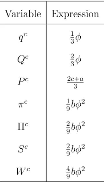
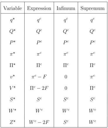
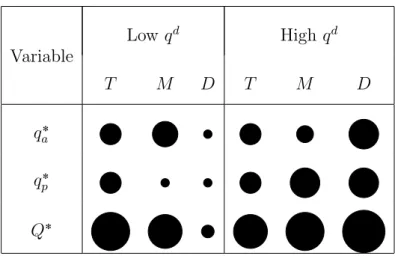
Conlisk (1996a) applies the notion of costly thinking to firms’ decisions. With the goal of understanding what is the effect of costly thinking on the dispersion of market variables, he states that firms, unable to costlessly choose the optimal quantity in each period, are equipped with a deliberation technology that leads them to choose a weighted average between an approximation to optimal output and a default quantity. Bounded rationality is manifested in the fact that the higher the effort put in finding a good approximation to the ideal output, the higher the thinking cost. The influence of this cost in firms’ choices is natural: a higher unit cost means less effort put on finding the ideal quantity and a chosen quantity closer to the default one. On the other hand, it can increase or attenuate market fluctuations, because its interaction with the rest of the model produces effects that go in opposite ways.

There are nt _{firms producing a homogeneous good in period} _t _{P t}₁_{, ...}_✉_{. In}

this period, firm i has to decide the quantity to produce, qt

i. Demand is given by

Q♣pt_{q ✏} _S_♣_a_✁_bpt_q ❄_Szt_{, where} _S _{represents market size and} _zt _{is a random}

variable, with zero mean and variance σ2

z. Firm i’s production cost in period t is

given byCt

i ♣qiq ✏ W q2

i 2wt

i, wherew

t

i is a random variable with meanµand variance

σ2

w. The quantity that maximizes profits in periodtiswtipt. As firms have to choose

(44)

t is qti r _✏

witE♣ptq. The quantity a boundedly rational firm i chooses to produce is

qt

i✝. This firm has a default quantity, corresponding to the long-run average quantity

produced by firms: qid ✏

E♣➦n_j_✏₁♣q✝_jqq

n . The firm does not know q t i r

, but is able to find ft

i ♣qti r

q ✏ qt i

r ut i

❄

ht i

, where ut

i is a zero mean random variable with variance

σu, and hti ➙ 0 is the level of deliberation of firm i in period t. However, the firm

pays a cost of c for each unit of ht

i chosen. Bounded rationality is also expressed

in the fact that the quantity chosen by firms is not what they consider to be the ideal quantity, but a weighted average of the perceived ideal and default quantities:

qit✝ ✏αtifit♣qit r_{q ♣}

1✁αtiqqit d

, where αti P r0,1s is to be chosen. The problem of firm

iin period t is then:

max

ht i,αti

E v_it ht_i, αt_i✟✟ ✏E ptqt_i✝ ht_i, α_it✟✁C_it qt_i✝ ht_i, αt_i✟✟✁ht_ic✟✟