Inverse modeling of soil characteristics from surface soil moisture observations: potential and limitations

(1)

HESSD

5, 95–145, 2008

Soil parameter inversion – potential

and limits

A. Loew and W. Mauser

Title Page

Abstract Introduction

Conclusions References

Tables Figures

◭ ◮

Back Close

Full Screen / Esc

Printer-friendly Version

Interactive Discussion

EGU Hydrol. Earth Syst. Sci. Discuss., 5, 95–145, 2008

www.hydrol-earth-syst-sci-discuss.net/5/95/2008/ © Author(s) 2008. This work is licensed

under a Creative Commons License.

Hydrology and Earth System Sciences Discussions

Papers published inHydrology and Earth System Sciences Discussionsare under open-access review for the journalHydrology and Earth System Sciences

Inverse modeling of soil characteristics

from surface soil moisture observations:

potential and limitations

A. Loew and W. Mauser

University of Munich, Department of Geography, Munich, Germany

Received: 28 November 2007 – Accepted: 8 December 2007 – Published: 23 January 2008

(2)

HESSD

5, 95–145, 2008

and limits

Title Page

Tables Figures

◭ ◮

Back Close

Full Screen / Esc

EGU

Abstract

Land surface models (LSM) are widely used as scientific and operational tools to sim-ulate mass and energy fluxes within the soil vegetation atmosphere continuum for nu-merous applications in meteorology, hydrology or for geobiochemistry studies. A re-liable parameterization of these models is important to improve the simulation skills.

5

Soil moisture is a key variable, linking the water and energy fluxes at the land surface. An appropriate parameterisation of soil hydraulic properties is crucial to obtain reliable simulation of soil water content from a LSM scheme. Parameter inversion techniques have been developed for that purpose to infer model parameters from soil moisture measurements at the local scale. On the other hand, remote sensing methods provide

10

a unique opportunity to estimate surface soil moisture content at diff_{erent spatial scales} and with diff_{erent temporal frequencies and accuracies. The present paper investigates} the potential to use surface soil moisture information to infer soil hydraulic characteris-tics using uncertain observations. Diff_{erent approaches to retrieve soil characteristics} from surface soil moisture observations is evaluated and the impact on the accuracy of

15

the model predictions is quantified. The results indicate that there is in general potential to improve land surface model parameterisations by assimilating surface soil moisture observations. However, a high accuracy in surface soil moisture estimates is required to obtain reliable estimates of soil characteristics.

1 Introduction

20

Soil moisture is a key link between the land surface and the atmosphere as it is an important parameter for many energy-balance related modeling applications such as numerical weather forecasting, climate prediction, radiative transfer modeling, global change modeling and other land process models (Owe et al., 2008). Land surface models have become indispensable tools to quantify and integrate the most important

25

(3)

HESSD

5, 95–145, 2008

and limits

Title Page

Tables Figures

◭ ◮

Back Close

Full Screen / Esc

EGU the use of these models requires model parameters to describe soil and vegetation

properties. At the same time these data are usually fragmented, are of diff_erent accu-racy and might change in time and space. Especially the temporal and spatial variabil-ity of soil hydraulic parameters (e.g. soil porosvariabil-ity, saturated conductivvariabil-ity) might have considerable eff_{ect on LSM simulations. Despite the progress that has been made in}

5

direct measurement of hydraulic characteristics of soils, these techniques remain rela-tively time consuming and therefore costly. However, direct or indirect observations of soil moisture dynamics might be used to infer soil hydraulic characteristics.

Various model calibration procedures have been developed that adjust model pa-rameter values to represent as closely as possible observations of a real system (Vrugt

10

et al., 2003). In order to automatically calibrate model parameters, algorithms defin-ing maximum likelihood functions for the measurement of the closeness between the model results and observations are defined and the model parameters are then opti-mised. A variety of global or local optimisation methods, such as the Shuff_{eld Complex} Evolution (SCE) algorithm (e.g.Duan et al.,1992;Yapo et al.,1998) or simulated

an-15

nealing (Thyer et al.,1999) have been used. Several studies have made an intercom-parison of these diff_{erent approaches (Madsen et al.,}_2002;_{Thyer et al.,}_1999).

While in situ measurements are restricted to small areas, remote sensing techniques are able to cover larger areas, which might off_{er the opportunity to infer soil} character-istics from these observation time series (Santanello et al.,2007). Numerous attempts

20

have been made to optimise LSM soil parameters using observations of soil water content and/or soil temperature (e.g.Gupta et al.,1999;Hogue et al.,2005;Liu et al., 2005).

Inverse modeling of soil hydraulic parameters is an established method to optimise the parameterization of land surface models (Vrugt et al.,2003,2005;Mertens et al.,

25

(4)

HESSD

5, 95–145, 2008

and limits

Title Page

Tables Figures

◭ ◮

Back Close

Full Screen / Esc

EGU constraints during the minimization procedure. Otherwise one might be able to find

nu-merous solutions for a model parameter set which all results in model predictions that coincident well with observations. This problem has been addressed as the equifinality problem in parameter estimation (Beven and Binley,1992;Beven and Freer,2001).

While the direct measurement of soil hydraulic characteristics is hampered by

com-5

plicated and costly measurements, indirect estimation of soil hydraulic properties is widely established. Soil pedotransfer functions (PTF’s) use soil variables that can be easily measured (soil texture, organic matter) to estimate soil hydraulic characteris-tics. There are a couple of reviews on PTF’s in the literature (Woesten et al.,2001; Woesten,1997;Rawls et al.,1991). Pedotransfer functions are typically statistical

re-10

lationships between soil textural parameters and the soil hydraulic characteristics and are estimated from the analysis of large soil data bases (Woesten et al.,1999;Batjes, 1996). However, the required soil texture information is available with diff_erent accu-racies at diff_{erent spatial scales. Global soil data is available e.g. from the FAO map} (FAO,1991) which provides soil texture data for the entire globe at very coarse spatial

15

scales (1:5 000 000), while much more detailed (e.g. scale 1:25 000) information might be available only for limited areas.

Recent studies have shown that the combination of land surface model simulations and soil moisture observations might be used to infer information on soil characteristics (de Lannoy et al.,2006;Vrugt et al.,2005;Lee,2005;Santanello et al.,2007). These

20

are based on continuous observations of soil moisture dynamics and corresponding land surface model simulations.

While in situ measurements provide accurate estimates of soil water content, con-tinuous records are limited to few locations on the globe (Robock et al., 2000). Re-mote sensing methods provide the opportunity to capture soil moisture dynamics at

25

(5)

HESSD

5, 95–145, 2008

and limits

Title Page

Tables Figures

◭ ◮

Back Close

Full Screen / Esc

EGU independent from atmospheric or illumination conditions which allows for a continuous

monitoring of the land surface. However, soil moisture retrievals from operational satel-lites are limited due to vegetation and surface roughness eff_{ects which might result in} ambiguous retrievals of soil water content. Wagner et al.(2007b) give a comprehen-sive overview about the applicability of diff_{erent remote sensing sensors for the retrieval}

5

of soil moisture for hydrological applications. The accuracy of the retrievals from mi-crowave sensors is highly dependent on the eff_{ect of vegetation on the one hand side} and the sensors specifications (frequency, polarizations, imaging geometry, spatial res-olution) on the other hand. The rms error of soil moisture retrievals might cover a wide range from 0.02 to 0.10 [cm3/cm3] (Loew et al.,2006;Wagner et al.,2007a).

10

Recent microwave and thermal infrared remote sensing techniques are only sensi-tive to the soil water content of the upper soil layer. Dependant on the observing system configuration, the sensitive layer is within the uppermost 1. . .10 cm, whereas the pen-etration depth is also dependent on the soil water content itself. However it has been shown that the assimilation of observations of surface soil moisture information into

15

hydrological models can result in improved predictions of soil water profiles (Enthekabi et al.,1994;Walker et al.,2001;Reichle and Koster,2005;Reichle et al.,2001); Loew, 20081. Future remote sensing missions as e.g. the forthcomingSENTINEL-1satellite (Attema,2005) will provide observations of the land at high spatial (<100 m) and high temporal (<3 days) resolutions which would allow for frequent and continuous

observa-20

tions of land surface dynamics. However it is likely that hydrological applications might only benefit from remote sensing observations when the derived information matches certain quality standards in terms of accuracy and observation frequency.

The present paper therefore examines the potential to infer soil information through inverse modeling by combining land surface model simulations with surface soil

mois-25

ture observations. The basic objective is to exploit time series of surface soil moisture information to improve land surface model parameterization schemes. The questions

1

(6)

HESSD

5, 95–145, 2008

and limits

Title Page

Tables Figures

◭ ◮

Back Close

Full Screen / Esc

EGU to be addressed are a) whether remote sensing derived surface soil moisture

infor-mation might be in general useful to infer soil characteristics, b) which accuracies of the remote sensing data and c) which temporal frequencies are needed to achieve an improved parameterization of a land surface model.

The analysis is made using an inverse modeling approach which minimizes the

de-5

viations between observations of surface soil moisture and model predicted water con-tent by altering land surface model parameters that describe the hydraulic characteris-tics of the soil.

The analysis is conducted using field data collected within the scope of the AGRISAR 2006 remote sensing campaign (Hajnsek et al.,2007) in Northern Germany. The

cur-10

rent state of modeling water movement in the unsaturated zone is described briefly in Sect. 2. The inverse modeling approach is introduced in Sect. 3 and data and used models are presented in Sect.4. The inverse modeling approach is given in Sect. 5 and results of the sensitivity analysis is presented in Sect.6.

2 Materials and methods

15

Consider a time-variant process modelΦ_{, that propagates the model state}x_i as

x_i=Φ_(x_i₋₁, p, u_i, w_i₋₁) (1)

wherei denotes the time,u_i is the vector of meteorological forcings andpis the model parameterization and w_i is a random process noise. Model parameters p have to be measured in the field or models are often calibrated for specific sites using local

20

ground observations. Mapping the model state space to the model output space, using the observation operatorH_i yields to the observationy_i as

y_i=H_ix_i+v_i (2)

whereasH_ix_i corresponds to model predicted measurements. These might be direct (e.g. soil moisture) or indirect (e.g. radiances of a satellite) measurements. In case that

(7)

HESSD

5, 95–145, 2008

and limits

Title Page

Tables Figures

◭ ◮

Back Close

Full Screen / Esc

EGU y_i is a direct observable of the model state vectorx_i ,H_i contains only elements of 0

and 1. The vectorv_i reflects the uncertainties of the measurement process. It might comprise uncertainties in the observation process, model forcing data, model physics and uncertainties in the model parameterization.

Most current approaches to data assimilation are derived from either a direct

ob-5

server or dynamic observer technique. While the direct observer approach assimilates sequentially information at various time steps of the model, the latter attempts to find the best fit between model simulations and observations over an entire time series of observations (Walker and Houser,2005). The dynamic observer technique might be formulated using either a strong or weak constraint assumption on the uncertainties of

10

the model simulationsw. In case of the strong constrained assumption, the process description of the physical modelΦ_{is considered to be perfect, while weak constraint} is where the uncertainties in the model formulation are taken into account as process noise.

In the present study we only focus on the uncertainties which are due to

measure-15

ment errors and model parameterization. Thus a perfect model (strong constraint) is assumed in the scope of the present study (w=_{0). The model parameter vector} p is assumed to be unknown and measurement errorsv are taken into account, assuming white noise.

2.1 Water movement in the unsaturated zone

20

The one-dimensional water movement in a partially saturated rigid porous medium might be described by the Richard’s equation as (Richards,1931)

∂θ(z, t) ∂t =

∂ ∂z

K(θ, z)

_{∂h(θ, z)}

∂z −1

(3)

where h is the soil water pressure head [m], θ is the volumetric water content [cm3/cm3], t is time [s], z is the spatial coordinate [m] and K is the unsaturated

hy-25

(8)

HESSD

5, 95–145, 2008

and limits

Title Page

Tables Figures

◭ ◮

Back Close

Full Screen / Esc

EGU andK(h) are generally non-linear functions of pressure headh. The Brooks and Corey

formulations relateK(h) andθ(h) to soil hydraulic characteristics as (Rawls and Brak-ensiek,1985;Brooks and Corey,1964)

θ−θ_r φ−θ_r =

_h

b

h λ

(4)

K(θ)=_K_s

_θ₋_θ

r

φ−θ_r 3+2λ

(5)

5

where λ is the pore size distribution index, θ_r is the residual water content, h_b the bubbling pressure head, φ the soil porosity and K is the fully saturated conductivity (θ=_{φ). Equation (4) is also often referred as water retention curve.}

2.1.1 Pedotransfer functions

Since direct measurements of soil hydraulic properties are time consuming,

expen-10

sive and not feasible at larger scales, alternative approaches to the estimation of soil hydraulic properties using pedotransfer functions (PTF) have been developed. PTF’s use easily measurable soil properties such as grain size or organic matter content to indirectly determine soil hydraulic characteristics. A variety of PTF’s have been pro-posed based on field measurements. As every PTF was developed on the basis of

15

a limited soil database, there is a lot of uncertainty in applying PTF’s to diff_{erent soil} conditions under which it was developed. It might be therefore reasonable to take into account these uncertainties in an optimisation procedure to infer hydrological model parameters.

Woesten et al. (2001) reviewed the current status of PTF’s and their accuracy and

20

(9)

HESSD

5, 95–145, 2008

and limits

Title Page

Tables Figures

◭ ◮

Back Close

Full Screen / Esc

EGU hydraulic conductivity and found that the PTF of Woesten (1997) performed best for

predicting the unsaturated hydraulic conductivity.

Given a set of soil texture parameters one might obtain diff_{erent values for the soil} hy-draulic properties which will directly reflect on the simulations of a hydrological model. Various PTF’s are therefore used in the present study. Table 1 summarizes the PTF’s

5

which are used for the diff_{erent model parameters within the present study.}

3 Inverse modeling of soil characteristics

3.1 Retrieval algorithm

In this section, the basis of the retrieval algorithm to estimate soil texture as well as soil hydraulic properties from surface soil moisture observations is introduced. The

10

retrieval is based on a numerical minimization of a cost function that accounts for the diff_{erences between the soil moisture predictions of a land surface model and surface} soil moisture observations. Two general cases are considered: 1) direct retrieval of soil hydraulic properties (hb, φ, θr, Ks, λ) and 2) retrieval of soil texture information as

sand and clay fractions, c, whereas soil hydraulic properties are estimated throughout

15

PTF’s.

Diff_{erent cost functions might be applied in that context using either only informations} about observation uncertainties or explicitly take into account potential uncertainties in the model parameters. In the latter case, the uncertainties of the model parameters are derived from diff_{erent PTF’s.}

20

3.2 Cost function derivation

(10)

HESSD

5, 95–145, 2008

and limits

Title Page

Tables Figures

◭ ◮

Back Close

Full Screen / Esc

EGU The unknown soil characteristics are represented by a vectorp =_{[λ, K}_s, θ_r, φ, h_b]T

Given a vector of soil moisture observationsy, the probability density function (pdf) of pconditioned by the observationsy is using Bayes’s theorem

P(p|y)∝P(y|p)P(p|p₀) (6)

whereP(p|p₀) is the pdf ofp given its prior estimatep₀. We assume that the error of

5

pis zero mean Gaussian, so that

p=_p₀+_ǫ_p ₍₇₎

where ǫ_p is the gaussian distributed parameter error. The probability function of p subject to a prior estimatep₀is then

P(p|p₀)∝exph−0.5(p−p₀)TG−1(p−p₀)i (8)

10

whereG is the diagonal covariance matrix. Additionally, the observations y are con-sidered to be aff_{ected by measurement errors}v ∈N(0,1). Gaussian error statistics is also assumed here. The probability of measuring a certainy given a model parameter setpis given by

P(y|p)∝exph−0.5(y −Hx(p))TS−1(y −Hx(p))i (9)

15

whereS is the diagonal covariance matrix. Substituting (8) and (9) into (6) yields the Bayesian likelihood function as

P(p|y)∝exph−0.5(y−Hx(p))TS−1(y−Hx(p))

−0.5(p−p₀)TG−1(p−p₀)i (10)

Since maximizing (10) is equivalent to minimize −ln(P(p|y)), the maximum likelihood

20

(11)

HESSD

5, 95–145, 2008

and limits

Title Page

Tables Figures

◭ ◮

Back Close

Full Screen / Esc

EGU 1993)

J=_0.5(y₋_Hx(p))TS−1(y−Hx(p))

+_0.5(p₋p₀)TG−1(p−p₀) (11)

Many diff_{erent minimization algorithms (e.g. Levenberg-Marquardt,} Nelder-mead-simplex) might be used to minimize the cost functionJ(Nelder and Mead,1965). When

5

no prior information on the model parametersp₀is available,P(p|p₀) can be dropped and (11) reduces to it’s first term which represents the traditional minimization of mean square error

J=_0.5(y₋_Hx(p))TS−1(y−Hx(p)) (12)

3.3 Accuracy assessment

10

To quantify the accuracy of the physical model predictions, the time series of model predictions and measurements are compared. Diff_{erent benchmarks are employed to} quantify the impact of the model parameterization on the model simulations. The used benchmarks are the root mean square error (rmse) [vol.%] and model effi_ciency_E _[−]. The comparisons are made on the basis of hourly values The rmse is calculated as

15

rmse= s

P

(y_i −Hx_i)2

n (13)

wherenis the number of observations andy andHxare the measured and predicted observations (e.g. soil moisture) respectively. The model effi_{ciency (E}_{) is estimated as} (Nash and Sutcliff_e,₁₉₇₀₎

E=₁₋ " P

(yi −Hxi)

2

P

(y_i −µ)2 #

(14)

20

(12)

HESSD

5, 95–145, 2008

and limits

Title Page

Tables Figures

◭ ◮

Back Close

Full Screen / Esc

EGU dynamic of the investigated parameter than a mean value. Perfect agreement between

the reference dataset and the simulations is achieved forE=_1.

4 Data and models

4.1 Land surface model

The Process Oriented Multiscale EvapoTranspiration model (PROMET) is used within

5

the present study to simulate water and energy fluxes. It is a family of land-surface-process-models which describe the actual evapotranspiration and water balance at diff_{erent scales, ranging from point scale, to micro- and mesoscale (Mauser and} Schaedlich,1998). The model consists of a kernel model which is based on five sub-modules (radiation balance, soil, vegetation, aerodynamic model, snow) to simulate

10

the actual water and energy fluxes and a spatial data modeller, which provides and organizes the spatial input data on the field-, micro- and macroscale. The simulations are made on an hourly basis.

Actual evapotranspiration is simulated within PROMET using the Penman-Monteith equation (Monteith, 1965). Canopy surface resistance is simulated as a function of

15

vegetation type using a resistance network approach (Baldocchi et al.,1987), while the soil resistance is estimated based on the approach ofEagleson(1978). A three layer soil model (0–10, 10–30, 30–150 cm) is used to represent the soil water fluxes. The soil water retention model ofBrooks and Corey (1964) is used to relate soil moisture content to soil suction head.

20

A ten layer vegetation model is used to convert the incoming radiation into fractions of shaded and sunlit leaves (Norman,1979). A detailed description of the model is given byMauser and Schaedlich(1998). A physical snow model extends PROMET to allow for simulations in cold climates (Strasser and Mauser,2001). Vegetation development is considered by prescribing the evolution of vegetation height, albedo and leaf area

25

(13)

HESSD

5, 95–145, 2008

and limits

Title Page

Tables Figures

◭ ◮

Back Close

Full Screen / Esc

EGU vegetation parameters.

PROMET simulations are based on GIS information as e.g. soil and land cover maps. Meteorological forcing data might be either provided from point like station measure-ments as well as gridded forcing fields. PROMET has been extensively validated in diff_{erent geographic regions (Upper Rhine Valley – 100 km}2_{, Bavarian Alpine Foreland}

5

– 20 000 km2, Upper Danube catchment – 76 000 km2, Weser catchment – 35 000 km2, India – 400 km2) using evapotranspiration measurements of micrometeorological sta-tions at the local scale and by comparison with thermal remote sensing informasta-tions at the regional scale (Mauser and Schaedlich, 1998;Ludwig and W.,2000;Pauwels et al.,2008); Loew, 20081.

10

4.2 Field data

4.2.1 Test site

The present study has been performed in the framework of the AgriSAR 2006 cam-paign, for which the test site was located in North-East Germany, approximately 150 km North of Berlin.Hajnsek et al.(2007) give a detailed description of the campaign. Only

15

a short description will be given here. The test site is based on a group of farms within a farming association covering approximately 250 km2. Field sizes are very large in this area, averaging between 2 and 2.5 km2. The main crops are winter wheat, winter barley, winter rape, corn, and sugar beet. The altitudinal range within the test site is approximately 50 m.

20

4.2.2 Meteorological data

The meteorological data to drive PROMET is obtained from an agrarmeteorological weather station (Goermin, 53.98 N/13.26 E). The station records meteorological data at 10 min frequency. The station is expected to provide best information on the local weather conditions.

(14)

HESSD

5, 95–145, 2008

and limits

Title Page

Tables Figures

◭ ◮

Back Close

Full Screen / Esc

EGU Meteorological inputs are the major model drivers, thus their accuracy directly

re-flects on the uncertainties of the model results. Loew 20081has shown that inaccurate estimates of meteorological input might result in large uncertainties of land surface model simulations. However reasonable results were found, when using local forcing data for the model simulations (Pauwels et al.,2008). This gives us confidence that

5

the strong constraint assumption of minor model error can be used within the present study. However, this assumption might probably not hold in case that forcing data might have much higher uncertainties.

4.2.3 Soil moisture measurements

Numerous field measurements and remote sensing data has been collected during the

10

investigation period which lasted from April to July 2006,. Continuous measurements of soil moisture were recorded within a wheat field. Soil water content was measured using TDR soil moisture probes (IMKO TRIME-ES), which were installed in depths of 5, 9, 15, 25 and 47 cm. The measurements were conducted within the period from 19 April 2006 (JD 109) to 06 July 2006 (JD 187). The wheat plants were at tillering stage

15

during the installation of the station and have reached the dough development stage at the end of the measurement period in accordance with the EUCARPIA code for cereals (Zadoks et al.,1974). Figure1shows the recorded soil moisture profiles. Soil moisture was homogeneous within the soil at the beginning of the measurement period, with values around 24% [cm3/cm3]. Except the uppermost soil layer (5 cm) shows slightly

20

reduced values (∼20% cm3/cm3). A first considerable precipitation event is observed between JD 136 and JD 145, where 20 mm precipitation were recorded. This results in an increase of the soil moisture content of the first 10 cm. A second precipitation event (27 mm) is observed between JD 148 and JD 156, which has also an impact on the soil moisture measurements at 25 cm depth. A 12 day period without precipitation follows.

25

(15)

HESSD

5, 95–145, 2008

and limits

Title Page

Tables Figures

◭ ◮

Back Close

Full Screen / Esc

EGU soil moisture values are observed from JD 110 to JD 125 (25% cm3/cm3). Afterwards,

the soil moisture of the lower soil layer shows an almost linear decrease until the end of the measurement period.

4.2.4 Soil information

Soil samples were taken in the investigated field at three diff_{erent locations. The}

sam-5

ples were analysed in the laboratory and the grain size of the soil particles was deter-mined. The total sand content is 57.2±1.3% and the clay content was estimated as 17.7±1.0%, whereas the major grain size is fine sand (200–63µm). The FAO soil map (FAO,1991) indicated a sand content of 51% and a clay content of 17% which is pretty close to the laboratory measurements.

10

5 Inverse modeling approach

The inverse modeling of soil characteristics is based on the comparison between sim-ulated and observed soil moisture time series. Model parameters are altered until best coincidence between model simulations and measurements is achieved. To infer soil characteristics from surface soil moisture observations the cost Functions (11) and

15

(12) are minimized using an iterative solver (Nelder-Mead-Simplex). Figure 2 shows the general data flow of the approach. Surface soil moisture observations are taken from TDR measurements. These are sampled with diff_{erent time intervals and various} observation errors v are assumed to mimic uncertainties in remote sensing derived surface soil moisture products. The PROMET model is used to simulate in a first step

20

the soil water content for a given investigation period, given an initial model parameter setp₀(initial guess). The model predictions (Hx) are then compared against the obser-vationsy. The parameter vectorpis iterated as long as no convergence is achieved. The minimization algorithm either minimizes directly the model soil hydraulic param-eters (solid line) or the soil texture data (dashed line) which is then used to estimate

(16)

HESSD

5, 95–145, 2008

and limits

Title Page

Tables Figures

◭ ◮

Back Close

Full Screen / Esc

EGU model parameters via the use of PTF’s.

Finally, the resulting model simulations are compared against the soil moisture ob-servations for the first (0–10 cm) and second (10–30 cm) PROMET soil layer. The TDR soil moisture measurements from 5 and 25 cm are used for that purpose respectively.

5.1 Model setup

5

5.1.1 Observation setup

It is expected that the temporal frequency as well as quality of the soil moisture ob-servations will aff_{ect the capability of estimating a reliable value for} _{p. To explicitly} investigate that impact, diff_{erent subsets are extracted from the surface soil moisture} measurements. These subsets are sampled with diff_{erent temporal frequencies to}

sim-10

ulate the case of diff_{erent observation frequencies of a sensor system. This sampling} was made at hourly and daily frequencies, increasing from one day to 14 days, resulting in a total of 15 diff_{erent time steps}_k.

Random gaussian error was added to each of these data sets to imitate various qual-ities of surface soil moisture observations. The standard deviation of the observation

15

error was set to 1, 2, 4, 6 vol.% [cm3/cm3], which covers a realistic range of uncertain-ties as it could be expected from remote sensing satellite data (Wagner et al.,2007a; Loew,2008).

5.1.2 Prior soil information

In case that prior information on soil properties is available, these might be used to

con-20

strain the minimization algorithm. This prior information can be derived either from field measurements or secondary sources as soil texture maps. The latter is used within the present study. The FAO soil map (FAO,1991), which is generally globally available, was used to estimate the first guess for the soil texture vectorm=[s, c]T. This initial guess

is used to estimate the background probability for the model parameter vectorpwhich

(17)

HESSD

5, 95–145, 2008

and limits

Title Page

Tables Figures

◭ ◮

Back Close

Full Screen / Esc

EGU requires the estimation ofp₀ and ǫ_p. These are obtained from a monte carlo based

sampling of the parameter space. As it is assumed that the FAO map might be highly uncertain, we assume a standard deviationσ_p which guarantees that also soil texture combinations which are far from the initial guess contribute to the calculation of p₀ andσ_p. This yields to the normal distributed ensemble matrixM_2xN=_[_m₁,m₂, . . . ,m_N] 5

whereN is the number of ensemble members and was assigned a value of 1000 in the present study.

To take into account the uncertainties of the PTF functions, diff_{erent PTF’s are} ap-plied for each model parameter. For each m, a set of different model parameters

(λ, Ks, hb, θr, φ) is obtained using PTF’s from different sources (Table7). This results 10

in an ensemble of 1000 values for the bubbling pressure headh_b, 1000 values for the pore size distribution indexλ, 4000 values forK_s, 3000 values for the porosity φand 2000 values for the residual water contentθ_r.

This ensemble of the model parameters is then used to calculate the mean and vari-ance for each model parameter which gives the prior guess on the model parameters

15

p₀and the associated covariance matrixGin Eq. (8). The obtained statistics for thep₀ parameters are given in Table3.

5.1.3 Open loop simulations

PROMET simulations are made using the prior information on soil parameters, as de-rived from either the laboratory measurements (LAB) or the FAO classification (FAO).

20

These simulations indicate the capabilities of the LSM to simulate soil water fluxes us-ing only a priori information without any observation data. To assess the impact of diff_{erent PTF’s on the model simulations, various PTF’s are applied to derive saturated} hydraulic conductivityK_sfrom the laboratory measurements.

The soil moisture simulations, using the laboratory measurements and FAO data for

25

(18)

underesti-HESSD

5, 95–145, 2008

and limits

Title Page

Tables Figures

◭ ◮

Back Close

Full Screen / Esc

EGU mate the soil water content in the spring period which might be attributed to the fact that

there was a snow cover in the study area until the end of March 2006 resulting in rather wet soil condition. PROMET simulations underestimated snow cover in spring and the soil moisture in the model therefore shows a negative bias. Nevertheless, the model shows a good performance also for the FAO data throughout the investigation period

5

which is due to the fact that the a priori information on the soil texture, taken from the FAO map, is in considerable agreement with the field measurements of grain size. In case that the FAO information would stronger deviate, much higher uncertainties in the model simulations can be expected. The soil moisture rms error as well as the model effi_{ciency for these open loop simulations are given in Table}₂_{for the upper (5 cm) and}

10

lower (25 cm) soil layer, respectively.

5.2 Model simulations

The prior model parameters p₀ are used to initialise PROMET. The simulations are made from 1 January 2005 to 30 June 2006. The first model year is used for model spin-up, while the comparisons and assimilation of soil moisture observations is only

15

done for the period from 20 April (JD 110) to 5 July 2006 (JD 186).

Only the surface soil moisture (5 cm) observations are used as measurement vari-able, while the deeper soil moisture observations are only used for accuracy assess-ment. Surface soil moisture observations were used every∆ttime steps which results in a multitemporal observation vector

20

y=[θ₁, θ₂, . . . , θ_N]T (15)

whereas θ_k corresponds to the surface soil moisture observations at time k . The PROMET model state vector x_i=[θ_L₁, θ_L₂, θ_L₃]T contains the PROMET soil moisture

predictions within the three diff_{erent soil layers. As only surface soil moisture} measure-ments are considered, the surface soil moisture predictions form the N-dimensional

25

multitemporal vector

(19)

HESSD

5, 95–145, 2008

and limits

Title Page

Tables Figures

◭ ◮

Back Close

Full Screen / Esc

EGU As the soil moisture measurements and the PROMET states represent the same

phys-ical parameter (soil moisture [vol.%], 0–10 cm depth), the observation operatorH in (2) reduces to a matrix with only 0 and 1 as elements. To analyse the eff_{ects of constraints} on the model parameters on the one hand side and to investigate the importance of prior soil texture information from secondary data on the other hand, the following

dif-5

ferent model scenarios are investigated:

– Scenario A: Direct determination of soil hydraulic parameters: the soil hydraulic characteristics are assumed to be unknown. The objective function is minimized by modifyingp=_{[λ, K}_s, φ, h_b, θ_r]T.

– Scenario B: Inverse modeling of soil texture using PTF’s without constraints on

10

model parameters: Sand and clay content are considered as free model parame-ters (m=[s, c]T ). Soil hydraulic characteristics are obtained from PTF’s, whereas

the uncertainties in the model parameters are not considered in the cost function (Eq.12)

– Scenario C: Inverse modeling of soil texture using PTF’s with constraints on model

15

parameters: same as scenario B, but uncertainties in the model parameterisation are considered in the cost function (Eq.11).

An appropriate initialisation of model parameters is important to minimize the risk that the minimization algorithm gets stuck in a local minima while searching for the optimal parameter set. To investigate the robustness of the parameter inversion approach, two

20

diff_{erent cases are investigated for the scenarios B and C. The first assumes that a} pri-ori information on soil texture is available from some source, while the other assumes that no a priori information is given. For the first the information from the FAO classifica-tion is used while standard values ofs=_{30% and}_c=_{30% are assumed for the second.} These scenarios are referred as (B1,C1) and (B2,C2), respectively. A summary of

25

model scenarios, used parameterisation and cost functions is given in Table3.

(20)

HESSD

5, 95–145, 2008

and limits

Title Page

Tables Figures

◭ ◮

Back Close

Full Screen / Esc

EGU diff_{erent measurements errors and 15 temporal sampling frequencies}∆twhich results

in 75 simulation runs per scenario and thus in a total number of 375 simulations.

6 Results

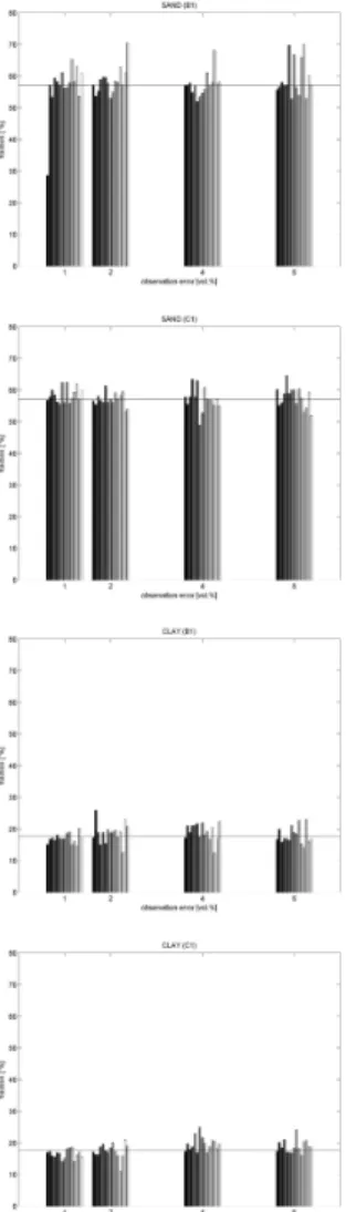
6.1 Inverse modeling of soil texture using PTF’s (constrained case)

The results of the inversion of soil texture (s, c) by integrating surface soil moisture

5

information is investigated in this section. Figure7shows the inversion results for clay and sand respectively for diff_{erent temporal frequencies and observation errors.} Ta-ble 4 summarizes the mean and standard deviation of the retrieval residues using the laboratory soil texture data as reference value. Given an appropriate initial guess for soil texture from the FAO map (B1,C1), the retrieved soil texture matches the sand and

10

clay content very well. The mean error is 0.54 (0.75) and 0.43 (0.38) for the B1 and C1 scenario respectively for clay (sand) content. No distinct dependency on the tem-poral sampling or observation error is observed. However, given a less accurate initial guess for soil texture (B2,C2), the uncertainties in the soil texture retrievals consider-ably increase. For low observation errors (1 vol.%), best retrieval results are observed.

15

When increasing the observation uncertainty, the uncertainties in the soil texture re-trievals also increase. Especially for high observation uncertainties large residues are observed, resulting in a mean error of−14.22 and−13.55 for the B2 and C2 simulation for sand respectively, while the residues of clay content are 2.01 and 3.06. This indi-cates that the retrievals give a higher weight to the silt content. From the analysis of the

20

field data it was found that fine sand and silt are the major fraction of the investigated soil. Thus the high deviations for sand do not necessarily imply a worse performance of the algorithm.

In both cases the consideration of uncertainties in the soil hydraulic parameters using (12) results in an improved prediction of the soil texture.

(21)

HESSD

5, 95–145, 2008

and limits

Title Page

Tables Figures

◭ ◮

Back Close

Full Screen / Esc

EGU 6.2 Impact of temporal sampling and observation error

It has been shown that the temporal sampling of the observations has a minor impact on the accuracy of the soil texture retrievals. Figure5shows the soil moisture profiles for four diff_{erent runs of the C1 scenario, using observations with daily, 4-day, 7-day and} 14-days sampling. It can be seen that there are only minor diff_{erences between the}

in-5

dividual model runs which indicates that the soil texture used for the model simulations matches quite well the expected value. However deficits in the model parameterization can also be observed. In case of dry soil conditions, the model is not able to sim-ulate the low soil moisture observations and saturate at a low soil moisture content of approximately 11 vol.%, while the observed values show a further decrease of the

10

soil water content. This might be explained by an underestimation of the soil hydraulic conductivity (Ks) using the PTF functions. Further discussion will be given in Sect. 6.3.

An increasing uncertainty of the observations results in positive bias of the model predictions as shown in Fig.6for the C1 scenario.

6.3 Error analysis

15

The error in the model soil moisture predictions is expressed for the investigation period in terms of the soil moisture rms error and model effi_ciency _{E. Figure} ₇ _{shows the} obtained rms errors and model effi_{ciencies for all combinations of observation errors} and sampling frequencies for the C1 scenario. The mean and standard deviation are 3.5 (0.3) and 0.62 (0.07) for the surface soil moisture rms error and model effi_ciency,

20

respectively. As it has been shown that the open loop simulations, using the FAO data as a reference, already provides good simulations for the investigated test site, the error benchmarks are normalized by the rms error and model effi_{ciency obtained from} the FAO open loop simulations (Table2). The normalized error values are also shown in Fig.7(bottom row) whereas unity indicates coincidence with the FAO result, values

25

(22)

HESSD

5, 95–145, 2008

and limits

Title Page

Tables Figures

◭ ◮

Back Close

Full Screen / Esc

EGU No systematic diff_{erences are observed between the di}ff_{erent model errors or}

tem-poral sampling rates. Most simulations show a similar accuracy than the open loop simulation which might be attributed to the fact that the FAO soil texture information already provides quite accurate estimates of the soil texture within the study area. Us-ing the FAO information as the initial guess (C1), no improvements are achievable by

5

assimilating the observation data into the model.

6.3.1 Constrained versus unconstrained

To evaluate the impact of using the diff_{erent cost functions (11) and (12), the results} of the B1 and C1 scenarios are compared. Figure8 shows the rms error and model effi_{ciency for the two cases respectively. Only minor di}ff_{erences are observed between}

10

the two approaches. The rms error is 3.5 vol.% in both cases and the mean model effi_{ciency is 0.61 and 0.62 for the unconstrained and constrained example respectively.} Figure 9shows the frequency distribution of the ratio of the two results for the rms error and model effi_{ciency respectively. Values below unity indicate lower rms error or} model effi_{ciency for the B1 scenario compared to the C1 scenario. The mean of the}

15

frequency distribution is 1.02 and 1.00 for the rms error and model effi_{ciency which} indicates again minor diff_{erences between the two modeling approaches. Thus the} consideration of model parameter uncertainties in the cost function does not result in an improvement of the model simulations skills in the present case..

6.3.2 Impact of a priori knowledge of soil characteristics

20

It has been shown that the a priori information on local soil texture, obtained from the FAO map, is within a reasonable range compared to the laboratory measurements. As a result, the integration of surface soil moisture information into the process model has a minor impact on the model parameterization. However, it might be expected that less accurate a priori information might be available at other places. To assess the

25

(23)

HESSD

5, 95–145, 2008

and limits

Title Page

Tables Figures

◭ ◮

Back Close

Full Screen / Esc

EGU approach, the scenarios C1 (B1) can be compared against C2 (B2). Figure10shows

the normalized rms error and model effi_{ciency with and without a priori soil texture} in-formation. While similar accuracies are achieved for observation errors below 4 vol.%, the accuracy of the model simulations becomes worse when increasing the observa-tion uncertainty. That indicates that the minimizaobserva-tion algorithm becomes more instable

5

in finding the optimal solution for higher uncertainties of the observations. However, in case of observations with uncertainties<4 vol.%, the obtained model predictions are in considerable agreement with those obtained from the open loop simulations which indicates that, given no first guess on soil texture, surface soil moisture informations might provide useful information to improve the soil parameterisation in those cases.

10

6.4 Inverse modeling of soil hydraulic parameters

In case that soil hydraulic parameters are directly inferred and no constraints are ap-plied to the retrieval by means of PTF’s (scenario A), diff_{erent simulation results might} be obtained. Figure7shows simulation results using diff_{erent observation frequencies} and an observation uncertainty of 1% vol. It is observed, that the model simulations

15

agree well with the TDR measurements. The soil moisture rms error is 1.7, 2.6, 2.1 and 2.9 for the daily, 4-day, 7-day and 14-day sampling interval respectively. Especially in case of low soil moisture values, the model simulations do much better match the observations which might be attributed by a better parameterization of the soil hydraulic conductivity. In case of daily observations, the model best captures the measured soil

20

moisture dynamics.

Figure 7 shows the rms error and model effi_{ciency for scenario A. It is seen, that} the obtained model simulations show a smaller rms error and higher model effi_ciency, compared to the simulations of scenario B and C. The mean value for the normalized rms error and model effi_{ciency are 0.73 and 1.11 respectively, indicating that the}

inte-25

gration of surface soil moisture information results in a more than 25% improvement compared to the open loop simulation (rms error).

(24)

HESSD

5, 95–145, 2008

and limits

Title Page

Tables Figures

◭ ◮

Back Close

Full Screen / Esc

EGU model parameters are within a reasonable physical range. Table5therefore compares

the retrieved soil hydraulic parameters against the direct predictions from the open loop simulations (FAO, laboratory) and corresponding literature values. The values taken fromRawls and Brakensiek (1985) are denoted in the first column and show a large variability in the soil parameters within a specific soil type. For the inversion results, the

5

mean and standard deviation are given.

The inversion results diff_{er from the parameters one obtains using the FAO or} lab-oratory soil texture information. However, the retrieved soil hydraulic parameters are within a reasonable range compared to the parameter range reported by Rawls and Brakensiek (1985). Except the saturated soil hydraulic conductivity slightly exceeds

10

the parameter range with a mean K_s value of 6.96 (cm/h). The higher values are re-quired to better capture the water movement in the soil column.

6.5 Impact on soil moisture profile

An improved simulation of surface soil moisture content will also reflect on the simula-tions of the soil water content in the deeper soil layers (10 - 30 cm). Thus an improved

15

parameterization of the surface soil characteristics might also aff_{ect the soil moisture} simulation skills of the deeper soil layers. Figure7shows measured and simulated soil moisture for the 10–30 cm layer for scenario A. Best model predictions are achieved for a daily assimilation which results in an rms error of 2.13 (cm3/cm3) and a model effi -ciency of 0.86 which corresponds to a slight improvement compared to the open loop

20

simulation (Table2). Figure7shows the normalized rms error and model effi_{ciency for} the deeper soil layer. The mean rms error and model effi_{ciency are 3.0 (cm}3_/cm3_{) and} 0.71 with standard deviations of 0.60 and 0.11 respectively. Improved simulations (nor-malized rms<1) are achieved only in case of frequent and accurate measurements. Approximately weekly observations with high accuracy (v=₁_{. . .}_{2 vol.%) are required}

25

(25)

HESSD

5, 95–145, 2008

and limits

Title Page

Tables Figures

◭ ◮

Back Close

Full Screen / Esc

EGU 2-day observation frequencies seem to be required to improve the model predictions.

A frequent coverage seems to be most important to capture the dry end conditions of the data set to be able to better find a parameter set that best represents the soil moisture dynamics.

However, it is emphasized again that the reference open loop soil moisture

simu-5

lation already matches well the observations. In case that the a priori information on soil texture might be much worse, the relative impact of integrating surface soil mois-ture data might be much higher and the model simulations might benefit more from observations with even higher uncertainties.

7 Conclusions

10

The present study has investigated the potential of using constrained and uncon-strained inverse modeling approaches to infer soil hydraulic characteristics. It was assumed that uncertainties in the physical model simulations are only due to uncer-tainties in the model forcing data or model parameterization, but not due the models process formulation.

15

Previous analysis of PROMET simulations (Pauwels et al.,2008); Loew 20081found that the model predictions of soil water and energy fluxes are in reasonable agreement with in situ data, which gives us confidence in that strong constraint assumption for the scope of this study. However, this assumption might be no longer valid if the model driving meteorological forcing data has a higher uncertainty. In these cases, the

addi-20

tional uncertainties of the forcing data and its impact on the model simulations will have to be taken into account within the analysis Loew (2008)1.

The conclusions that can be drawn from the analysis of the conducted experiment are

1. Constrained as well as unconstrained model parameter calibration strategies

25

(26)

HESSD

5, 95–145, 2008

and limits

Title Page

Tables Figures

◭ ◮

Back Close

Full Screen / Esc

EGU 2. Soil grain size might be infered by inverse modeling of surface soil moisture data.

3. However, an appropriate initial guess of the soil texture is critical for a robust estimate of soil characteristics. Otherwise the inversion algorithm is likely to get stuck in a local minima in case of observation errors>4 vol.%.

4. The direct inversion of soil hydraulic parameters results in realistic model

parame-5

ter retrievals. The direct calibration of model parameters outperforms the indirect approach using PTF’s.

5. An improved model parameterization using surface soil moisture information might be used to improve the model predictions also in the deeper soil layer. Observations frequencies less than a week are required to improve the model

10

simulations compared to the open loop simulation in the present case to best capture dry soil moisture conditions.

The results indicate that there is potential in using (uncertain) surface soil moisture information to improve root zone soil moisture predictions throughout a better param-eterization of the physical model. However, the conclusions are limited to the data

15

set used in the present investigation. In case that the soil is layered and not as ho-mogeneous as in case of the present test site, the integration of surface soil moisture information might fail to improve the model predictions. Only minor dependency on the temporal sampling was observed using PTF’s. However it was found that the prediction of deeper soil water content benefits from a higher sampling rate of the observations.

20

Using observations with frequencies below one week show improved model skills. As the FAO soil texture information is available at global scale, a priori information on soil properties might be available from that data set. However, there might be con-siderable diff_{erences between the FAO information and the local soil texture due to} the rather coarse scale of that map. It is therefore expected that much worse

perfor-25

(27)

HESSD

5, 95–145, 2008

and limits

Title Page

Tables Figures

◭ ◮

Back Close

Full Screen / Esc

EGU The meteorological forcing data which was used for the model simulations was based

on local measurements and can therefore be considered as a reliable input for the model simulations. However Loew (2008)1has shown that considerable diff_{erences in} the model simulations are observed when meteorological data is taken from a station 20 km apart from the test site which might complicate the inversion of soil

character-5

istics from the surface soil moisture observations. A simultaneous compensation for uncertainties in model forcings as well as in the model parameterisation would then be required. The use of sequential data assimilation techniques as e.g. the Ensem-ble Kalman Filter (Evensen,2003) with augmented state vectors might be used in that context together with frequent observations. Forthcoming satellite missions as the

10

SENTINEL-1 mission will allow for that frequent coverage at high spatial resolutions.

Acknowledgements. The work has been supported by the European Space Agency (ESA) under contract 19569/06/NL. Field data was collected within the scope of the AGRISAR 2006 campaign funded by ESA which is gratefully acknowledged.

References

15

Attema, E.: GMES Sentinel-1 Mission Requirements Document, Tech. rep., ESA publication, Issue1.4, ES-RS-ESA-SY-0007, 2005. 99

Baldocchi, D., Hicks, B., and P., C.: A canopy stomatal resistance model for gaseous deposi-tions to vegetated surfaces., Atm. Environ. 1987, 21(1), 91–101, 1987. 106

Batjes, N.: Development of a world data set of soil water retention properties using pedotransfer

20

rules, Geoderma, 71(1–2), 31–52, 1996. 98

Beven, K. and Binley, A.: The future of distributed models: model calibration and uncertainty prediction, Hydrol. Processes, 6, 279–298, 1992. 98

Beven, K. and Freer, J.: Equifinality, data assimilation, and uncertainty estimation in mechanis-tic modelling of complex environmental systems, J. Hydrol., 249, 11–29, 2001. 98

25

Brooks, R. and Corey, A.: Hydraulic properties of porous media, Tech. rep., Hydrology paper 3. Colorado State University, Fort Collins, Colorado, 1964. 102,106

(28)

HESSD

5, 95–145, 2008

and limits

Title Page

Tables Figures

◭ ◮

Back Close

Full Screen / Esc

EGU estimation for soil moisture profiles by an ensemble Kalman filter: Effect of assimilation depth

and frequency, Water Resour. Res., 43, 1–15, 2006. 98

Cosby, B. J., Hornberger, G. M., Clapp, R. B., and Ginn, T.R.: A statistical exploration of the relationships of soil moisture characteristics to the physical properties of soils, Water Resour. Res., 20, 682–690, 1984.126

5

Duan, Q., Soorooshian, S., and Gupta, V.: Effective and efficient global optimisation for con-ceptual rainfall-runoffmodels, Water Resour. Res., 28(4), 1015–1031., 1992. 97

Dubois, P., van Zyl, J. J., and Engman, T.: Measuring soil moisture with imaging radars, IEEE Trans. Geosc. Rem. Sens, 33, 915–926, 1995.98

Eagleson, P.: Climate, soil, and vegetation, simplified model of soil-moisture movement in

10

liquid-phase, Water Resour. Res., 14(5), 722-730, 1978. 106

Enthekabi, D., Nakamura, H., and Njoku, E.: Solving the inverse problem for soil moisture and temperature profiles by sequential assimilation of multifrequency remotely sensed obersva-tions, IEEE Trans. Geosc. Rem. Sens, 32(2), 438–448, 1994.99

Evensen, G.: The Ensemble Kalman Filter: theoretical formulation and practical

implementa-15

tion, Ocean Dynamics, 53, 343-367, doi:10.1007/s10236-003-0036-9, 2003. 121

FAO: The digitised soil map of the world, World Soil Resources Report, 67(1), 1991. 98,109,

110

Gupta, H. V., Bastidas, L. A., Sorooshian, S., Shuttleworth, W. J., and Yang, Z. L.: Parameter estimation of a land surface scheme using multi-criteria methods, J. Geophys. Res., 104,

20

19 491–19 504, 1999. 97

Hajnsek, I., Bianchi, R., Davidson, M., DUrso, G., Gomez-Sanchez, J., Hausold, A., Horn, R., Howse, J., Loew, A., Lopez-Sanchez, J., Ludwig, R., Martinez-Lozano, J., Mattia, F., Miguel, E., Moreno, J., Pauwels, V., Ruhtz, T., Schmullius, C., Skriver, H., Sobrino, J., Timmermans, W., Wloczyk, C., and Wooding, M.: AgriSAR 2006 Airborne SAR and Optics Campaigns

25

for an improved monitoring of agricultural processes and practices, European Geoscience Union (EGU), General Assembly, 15–20 April 2007, Vienna, Austria, 2007.100,107

Hogue, T. S., Bastidas, L., Gupta, H., Sorooshian, S., Mitchell, K., and Emmerich, W.: Evalua-tion and transferability of the Noah land surface model in semiarid environments, J. Hydrol., 6, 68–84, 2005. 97

30

Lee, D.-H.: Comparing the inverse parameter estimation approach with pedo-transfer function method for estimating soil hydraulic conductivity, Geosci. J., 9(3), 269–276, 2005. 98

(29)

HESSD

5, 95–145, 2008

and limits

Title Page

Tables Figures

◭ ◮

Back Close

Full Screen / Esc

EGU surface and atmospheric parameters of a locally coupled model using observational data, J.

Hydrometeorol., 6, 156–172, 2005. 97

Loew, A.: Impact of surface heterogeneity on surface soil moisture retrievals from passive microwave data at the regional scale: the Upper Danube case, Rem. Sens. Env., 112, 231– 248, doi:10.1016/j.rse.2007.04.009, 2008. 98,110

5

Loew, A., Ludwig, R., and Mauser, W.: Derivation of surface soil moisture from ENVISAT ASAR WideSwath and Image mode data in agricultural areas, IEEE Trans. Geosc. Rem. Sens, 44(4), 889–899, 2006. 98,99

Ludwig, R. and Mauser, W.: Modelling catchment hydrology within a GIS-based SVAT-model framework, Hydrol. Earth Syst. Sci., 4(2), 239–249, 2000. 107

10

Madsen, H., Wilson, G., and Ammentorp, H.: Comparison of different automated strategies for calibration of rainfallrunoffmodels, J. Hydrol., 261(1–4), 48–59, 2002. 97

Mauser, W. and Schaedlich, S.: Modelling the spatial distribution of evapotranspiration using remote sensing data and PROMET, J. Hydrol., 213, 250–267, 1998. 106,107

Mertens, J., Stenger, R., and Barkle, G. F.: Multiobjective Inverse Modeling for Soil Parameter

15

Estimation and Model Verification, Vadose Zone Journal, 5, 917-933, 2006. 97

Monteith, J.: Evaporation and the environment, Proc. Symposium of the society of exploratory biology, 19, 205–234, 1965. 106

Nash, J. and Sutcliffe, J.: River flow forecasting through conceptual models part I - A discussion of principles, J. Hydrol., 10(3), 282–290, 1970. 105

20

Nelder, J. and Mead, R.: A simplex method for function minimization, The Computer Journal, 7, 308–313, 1965. 105

Norman, J., Barfield, B., and Gerber, J.: Modification of the Aerial Environment of Plants, chap, Modelling the complete crop canopy, Am. Soc. Agr. Eng., 249–277, 1979. 106

Owe, M., de Jeu, R., and Holmes, T.: Multi-Sensor Historical Climatology of Satellite-Derived

25

Global Land Surface Moisture, J. Geophys. Res., in press, 2008.96

Pauwels, V., Timmermans, W., and Loew, A.: Study of the water and energy budget during AGRISAR 2006, J. Hydrol., in press, 2008. 107,108,119

Pulliainen, J., Karna, J.-P., and Hallikainen, M.: Development of geophysical retrieval algorithms for the MIMR, IEEE Trans. Geosc. Rem. Sens, 31(1), 268–277, 1993. 104

30

(30)

HESSD

5, 95–145, 2008

and limits

Title Page

Tables Figures

◭ ◮

Back Close

Full Screen / Esc

EGU Rawls, W., Gish, T., and Brakensiek, D.: Estimating soil water retention from soil physical

properties and characteristics, Adv. Soil Sci., 16, 213–234, 1991. 98

Reichle, R., Entekhabi, D., and McLaughlin, D.: Variational Data assimilation of microwave radiobrightness observations for land surface hydrology applications, IEEE Trans. Geosc. Rem. Sens, 39(8), 1708–1718, 2001.99

5

Reichle, R. H. and Koster, R.: Global assimilation of satellite surface soil moisture retrievals into the NASA catchment land surface model, Geophys. Res. Lett., 32, L02404, doi:10.1029/ 2004GL021700, 2005.99

Richards, L.: Capillary conduction of liquids through porous mediums, Physics, 1, 318–333, 1931. 101

10

Robock, A., Vinnikov, K. Y., Srinivasan, G., Entin, J. K., Hollinger, S. E., Speranskaya, N. A., Liu, S., and Namkha, A.: The Global Soil Moisture Data Bank, B. Am. Meteor. Soc., 1281–1299, 2000. 98

Santanello, J. A., Peters-Lidard, C. D., Garcia, M. E., Mocko, D. M., Tischler, M. A., Moran, S., and Thoma, D.: Using remotely-sensed estimates of soil moisture to infer soil texture and

15

hydraulic properties across a semi-arid watershed, Rem. Sens. Env., 110, 79–97, 2007. 97,

98

Saxton, K. E., Rawls, W. J., Romberger, J. S., and Papendick, R. I.: Estimating generalized soil-water characteristics from texture, Soil Sci. Soc. Am. J., 50, 1031–1036, 1986.126

Scheinost, A. C., Sinowski, W., and Auerswald, K.: Regionalization of soil water retention

20

curves in a highly variable soilscape, I.: Developing a new pedotransfer function, Geoderma, 78, 129–143, 1997.126

Strasser, U. and Mauser, W.: Modelling the spatial and temporal variations of the water balance for the Weser catchment 1965–1994, J. Hydrol., 254(1–4), 199–214, 2001. 106

Thyer, M., Kuczera, G., and Bates, B.: Probabilistic optimisation for conceptual rainfallrunoff 25

models: a comparison of the shuffl_{ed complex evolution and simulated annealing algorithms,}

Water Resour. Res., 35(3), 767–773, 1999. 97

Vrugt, J., Gupta, H., Bastidas, L., Bouten, W., and Soorooshian, S.: Effective and efficient algorithm for multiobjective optimiztion of hydrological models, Water Resour. Res., 39(8), 2003. 97

30