BARKER, CLAYTON ADAM. The Orthogonal Interactions Model for Unreplicated Factorial Experiments. (Under the direction of Leonard Stefanski and Jason Osborne.)
Unreplicated factorial experiments arise frequently in practice because of limited
resources. When fitting the standard ANOVA model to data from unreplicated
experi-ments, the data are not sufficient to estimate the interaction terms and error variance,
thus limiting the possible inferences. In experiments such as crop yield trials,
inves-tigators are interested in estimating interactions but are unable to form replications.
Existing methods, such as Tukey’s one-degree-of-freedom model and the AMMI model,
fit constrained interactions which allow for the error variance estimation.
We present theorthogonal interactions (OI) model for unreplicated factorial exper-iments. The model frees degrees of freedom for error by assuming that the main effects
are orthogonal to the interactions. Through simulation we find that approximate F -statistics are appropriate in testing for main effects and interactions. The likelihood
ratio test to compare the OI model to the ANOVA model leads to high Type I error
rates, so we use a simulation corrected likelihood ratio test. Two real data sets (one
with replication, one without) suggest that the OI model is appropriate for real data.
In working with the OI model and the existing models, we found a need for
re-liable degrees of freedom for complex statistical models. The resampling method for estimating degrees of freedom is motivated by the linear model, where there is a linear
relationship between expected sums of squares and the variance of errors added to the
response. Through simulation, we find that the resampling method provides reliable
Unreplicated Factorial Experiments
by
Clayton Barker
a dissertation submitted to the graduate faculty of
north carolina state university
in partial fulfillment of the
requirements for the degree of
doctor of philosophy
statistics
raleigh, nc
December 1, 2006
approved by:
Dr. Leonard Stefanski (co-chair) Dr. Jason Osborne (co-chair)
Clay Barker was born on December 15, 1978 to Kaye and Terry Barker in Tampa,
Florida. After living in Tampa; Myrtle Beach, South Carolina; and Atlanta, Georgia;
the Barker family settled in Chapel Hill, North Carolina in January 1987. In 1997,
Clay graduated from Chapel Hill High School and began his undergraduate work at
North Carolina State University as an applied mathematics major. In May 2001,
Clay completed his Bachelor of Science degree in applied mathematics with a minor in
statistics. Clay chose to stay at NCSU to pursue a graduate degree in statistics. He
received his Master of Statistics degree in 2003 and his doctoral degree in 2006 under the
direction of Dr. Leonard Stefanski and Dr. Jason Osborne. Clay received the Gertrude
Cox Outstanding Ph.D. candidate award in 2004. As a graduate student, Clay had
the opportunity to serve as teaching assistant for undergraduate and graduate level
courses, serve as a research assistant on a project with the Environmental Protection
First of all, I must thank my advisors Dr. Leonard Stefanski and Dr. Jason Osborne
for their guidance and support throughout my graduate career. They provided me
with a tremendous amount of knowledge while still giving me the freedom to discover
things on my own. They are excellent statisticians and people, and I am fortunate to
have had the opportunity to work with them. I would also like to thank my committee
members for their contributions to this document. Dr. Sastry Pantula and Dr. Bill
Swallow have also provided support throughout my graduate career. I must also thank
Terry Byron and Adrian Blue for all that they do for our department. We are lucky
to have such excellent faculty and staff in our department.
I have endured stressful days and long nights as a graduate student, but I have not
had to go about it alone because of a strong support group of friends. I am fortunate
to have gone through grad school with a fine group of classmates and officemates.
Besides helping me with courses and research, I have enjoyed trips to Mitch’s, NCSU
athletics, trips to the gym, as well as many other activities with friends I have met in
the department. I am grateful for Amanda, Darryl, Hugh, Jimmy, Joe, Justin, Kirsten,
Lavanya, Matthew, Michael, Mike, Paul, Ross, Steve, and Theresa, all of whom I met
in the graduate program. When times got tough in the office, we often found that a
makeshift game consisting of a ball and a trashcan was sufficient to raise our spirits.
I must also thank my former roommate Brad who I met during my freshman year
at NCSU. Brad has been a good friend and he has helped make my college years a lot
graduate studies. Kimberly has seen me at my best and my worst, but she has always
loved me, supported me, and given me the confidence to reach my goals. I appreciate
her patience and understanding through this process.
Most importantly, I must thank my family for supporting me in everything I have
done. My brother Jason attended NCSU for his undergraduate and graduate studies
as well, and I was very fortunate that our time at NCSU overlapped for several years.
Football games, basketball games, trips to the gym, movies, concerts, and countless
other activities; I could not have gotten through this process without his advice and
I would not be the person I am today without his friendship. Finally, and most
importantly, I would like thank my parents. They believe in me and encourage me in
everything that I pursue. My parents have provided me with a tremendous amount
of support, an example of how to balance family and career, and a great set of genes
among other things. Without the love and support of my family, I would have never
List of Tables . . . ix
List of Figures . . . xi
1 The Orthogonal Interactions Model . . . 1
1.1 Motivation . . . 2
1.2 Orthogonal Interactions Model Definition . . . 4
1.3 Existing Models . . . 6
1.4 Fitting the Orthogonal Interactions Model . . . 10
1.4.1 Fitting the OI Model by Reparameterization . . . 11
1.4.2 The Profile Likelihood Method for Fitting the OI Model . . . . 15
1.5 Fitting the Existing Models . . . 19
1.5.1 Fitting the AMMI model . . . 20
1.5.2 Fitting the Tukey One-Degree-of-Freedom Model . . . 22
1.6 Inference Issues . . . 22
1.6.1 Inference and the Orthogonal Interactions Model . . . 23
1.6.2 Inference and Existing Methods . . . 32
1.7 Recognizing Data from the Orthogonal Interactions Model . . . 36
1.8 Testing the Orthogonality Assumptions . . . 41
1.8.3 Testing the OI Model for Unreplicated Data . . . 56
1.8.4 Determining Why the Orthogonality Assumptions are Violated . 60 1.9 Example Fits . . . 62
1.9.1 Metal Shear Strength Data . . . 62
1.9.2 Soil Data . . . 66
1.10 Simulation Results . . . 74
1.10.1 Variance Estimation . . . 74
1.10.2 Testing Simulations . . . 77
1.11 Conclusions . . . 81
2 A Resampling Based Method For Estimating Degrees of Freedom 83 2.1 Motivation . . . 84
2.2 Resampling Method for Estimating Degrees of Freedom . . . 89
2.3 Resampling Degrees of Freedom and the Familiar Models . . . 95
2.4 Resampling Degrees of Freedom and the AMMI Model . . . 101
2.5 Discussion . . . 109
Literature Cited . . . 110
Appendix . . . 113
A Technical Details . . . 113
1.1 Estimated Error Degrees of Freedom for a × b Data Using Rank Method. 25
1.2 Rank DF and Adjusted Rank DF for 6 × 6 OI Data . . . 26
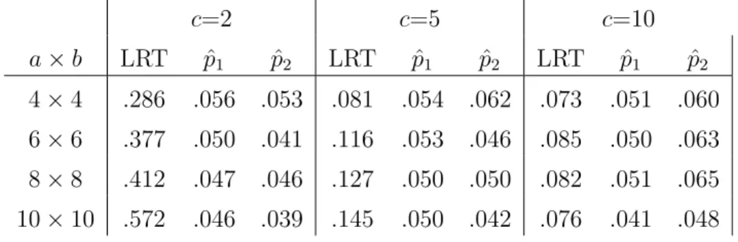
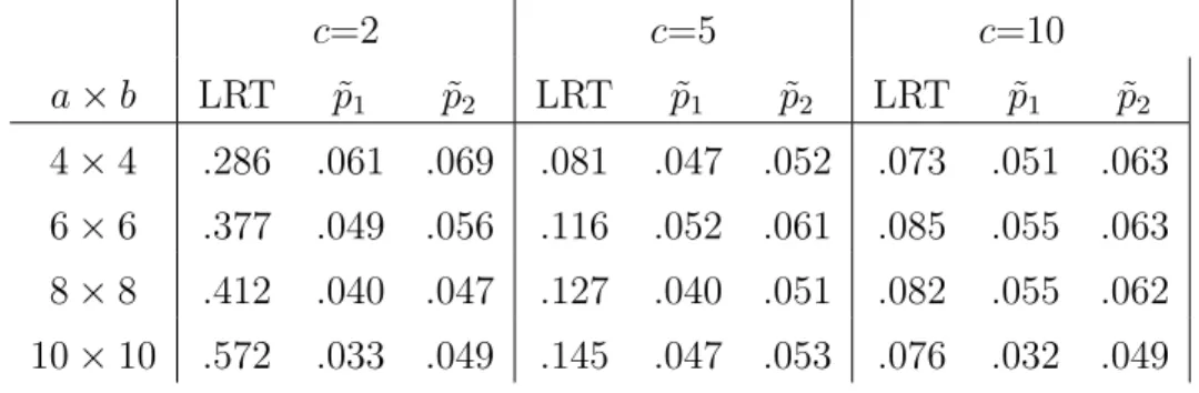
1.3 Type I Error Rates for Bootstrap Corrected LRT of Orthogonality As-sumptions for a×b Data with c Replicates (Monte Carlo SE: 6.9E-3) . 47 1.4 Type I Error Rates for Noise Corrected LRT of Orthogonality Assump-tions for a×b Data with c Replicates (Monte Carlo SE: 6.9E-3) . . . . 52
1.5 Full ANOVA Fit of Metal Strength Data. . . 63
1.6 Orthogonal Interactions Fit of Metal Strength Data. . . 63
1.7 Orthogonal Interactions Fit of Soil Data (Resampling DF) . . . 68
1.8 AMMI(2) Fit of Soil Data (Resampling DF) . . . 68
1.9 Tukey 1-DF Fit of Soil Data. . . 69
1.10 Several Different Degree of Freedom Estimates For Orthogonal Interac-tions Model and AMMI(2) Analysis of Soil Data. . . 72
1.11 Simulated Error Variance Estimates for Orthogonal Interactions Model (σ2 = 1) . . . . 75
1.12 Simulated Error Variance Estimates for Data Generated without Main Effects or Interactions (σ2 = 1) . . . . 76
2.1 Expected SS and Expected MS for Mixed Effect Model . . . 87
2.2 Summary Table of Average Sums of Squares . . . 91
Defined by (2.8) . . . 101 2.5 Summary of Error Variance Estimation for AMMI Data (σ2 = 1) . . . 107
1.1 Mean Profiles: (a) OI Model (b) ANOVA Model . . . 37 1.2 Biplots of: (a) Tukey Data(b) Linear-bilinear Data . . . 40 1.3 Histogram of Simulated Unadjusted LRT p-values . . . 48 1.4 Histograms of Bootstrap Adjusted p-values for Tests Based on: (a) ˆp1
(b) ˆp2 . . . 49
1.5 Histogram of Unadjusted Likelihood Ratio Test Statistic and χ25 Distri-bution . . . 50 1.6 Histogram of Bootstrap Adjusted Likelihood Ratio Test Statistic and χ25
Distribution . . . 51 1.7 Histograms of Noise Adjusted p-values for: (a) Adjusted LRT (b)
Em-pirical Test . . . 54 1.8 Histogram of Noise Adjusted Likelihood Ratio Test Statistic andχ2
5
Dis-tribution . . . 55 1.9 Power Curves of Test (1.27) Using Two Different Empirical Methods
(Monte Carlo SE: 6.9E-3) . . . 58 1.10 Power Curves of Adjusted Empirical Tests of (1.27) when Parameters
do not Satisfy Orthogonality Assumptions (Monte Carlo SE: 6.9E-3). . 59 1.11 Metal Strength Prediction Profiles- (a) OI Model(b) ANOVA . . . 65 1.12 Scatterplot of ANOVA Predictions versus OI Model Predictions for Metal
1.15 Soil Data Profiles- (a) OI Predictions (b) ANOVA Predictions (c) Raw Data . . . 71 1.16 Scatterplot of AMMI(2) Predictions versus OI Model Predictions for Soil
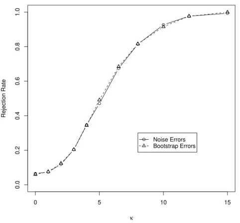
Data . . . 73 1.17 Power of Main Effect F-tests Formed Using Both Degree of Freedom
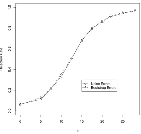
Methods (Monte Carlo SE: 9.7E-3) . . . 79 1.18 Power of Interaction F-tests Formed Using Both Degree of Freedom
Methods (Monte Carlo SE: 9.7E-3) . . . 80
2.1 Average Error Sum of Squares as a Function of Added Error Variance . 93 2.2 Power of Main Effect F-tests using True DF and Resampling DF (Monte
Carlo SE: 6.9E-3) . . . 99 2.3 Power of Interaction F-tests using True DF and Resampling DF (Monte
Carlo SE: 6.9E-3) . . . 99 2.4 Rejection Rates for Interaction F-tests using Various Degree of Freedom
Methods with the AMMI Model (Monte Carlo SE: 6.9E-3) . . . 104 2.5 Rejection Rates of Main Effect F-tests using Various Degree of Freedom
The Orthogonal Interactions Model
The standard two-factor analysis of variance model with A at a levels, B at b levels, and creplicates per factor level combination (FLC) is
Yijk =µ+αi+βj+γij +ǫijk, (1.1)
where Piαi = 0, Pjβj = 0, Piγij = 0 for all j, Pjγij = 0 for all i, and ǫijk are independent and identically distributed N(0, σ2) variates. If c = 1, the case of no replication, the data are not sufficient to estimate the interaction terms, γij, and the error variance σ2, thus limiting the possible inferences. In experiments such as crop yield trials, investigators are interested in main effects as well as interactions. Because
of expenses or other limitations, obtaining replicates is not always an option. An
alternative is to estimate a set of constrained interactions, thus providing some degrees
of freedom for error variance estimation. An extreme version of this strategy assumes
that all γij = 0, thereby providing (a−1)(b−1) degrees of freedom for estimating σ2
in this case. Note that in this case, (a−1)(b−1) additional constraints are imposed on the interactions. Other versions of this strategy are at the heart of Tukey’s one degree
of freedom test of additivity as well as the so-called AMMI (additive main effects and
multiplicative interactions) model used extensively in agricultural research. We discuss
for the usual ANOVA model that will allow for estimation of the interaction terms
while providing degrees of freedom for error in the case of no replication and compare
our new model to existing models.
The remainder of this chapter is organized as follows. In Section 1.1 we provide the
motivation for the orthogonal interactions model with a formal definition of the model
in Section 1.2. Then in Section 1.3 we present existing models that fit constrained
in-teractions to unreplicated two-factor models. We provide two approaches to fitting the
orthogonal interactions model in Section 1.4 and details for fitting the existing models
in Section 1.5. Inference is considered in Section 1.6 for the orthogonal interactions
model as well as the existing models. In Section 1.7 we discuss how to recognize data
from the orthogonal interactions model and in Section 1.8 we discuss testing the
appro-priateness of the orthogonality assumptions for both replicated and unreplicated data.
We fit the orthogonal interactions model and the existing models to several real data
sets in Section 1.9. In Section 1.10 we use simulations to investigate the performance
ofF-tests and to investigate the error mean square as an error variance estimator when using the orthogonal interactions model.
1.1
Motivation
We propose a set of constraints that allow the estimation of interaction terms and
error variance for two-factor ANOVA data without replication. The new constraints
model with interactions is written
Yijk =µ+αi+βj +γij +ǫijk i= 1, ..., a; j = 1, ..., b; k= 1, ..., c; (1.2)
where
αi iid∼ N(0, σa2) ,βj iid∼ N(0, σb2) ,γij iid∼ N(0, σg2) , andǫijk iid∼N(0, σ2e).
Furthermore, it is assumed that the main effects and interactions are all mutually
inde-pendent. This assumption of independence is equivalent to the assumption underlying
random effect models for crossed designs, that Cov(αi, γij) = 0 for all i and j, which in turn implies that
E(αiγij) = 0 for alli and j,
because E(αi) = E(γij) = 0. A similar argument can be made with the βjγij terms. These assumptions of independence imply that the main effects vectors are orthogonal
to the rows/columns of the interaction matrix in expectation. The assumption of main
effects being orthogonal to interactions can be carried over to the fixed effects ANOVA
model. These ideas from the random effects ANOVA model provide motivation for the
orthogonal interactions (OI) model.
Comparing the assumptions of the fixed effects model (1.1) to those of the random
effects model (1.2), we see a natural correspondence between effect sample moments in
the fixed effects model and the population moments in the random effects model:
1 a
X
i
1 b
X
j
βj = 0 corresponds to E(βj) = 0,
1 ab
X
j
X
i
γij = 0 corresponds to E(γij) = 0.
The correspondences in (1.3) are the ‘natural’ correspondences that one considers upon
comparing (1.1) and (1.2). However, the random effects model has the additional
population assumption that E(αiγij) = E(βjγij) = 0. The fixed effect model finite
population versions of these are:
1 b
b
X
j=1
βjγij = 0, for all i; and 1 a
a
X
i=1
αiγij = 0, for all j. (1.4)
The constraints in (1.4) have not been previously imposed on the fixed effects model.
However, imposing (1.4) in the fixed effects model frees degrees of freedom for
estimat-ing σ2. In the c= 1 case, imposing (1.4) allows for the estimation of the γij as well as σ2.
1.2
Orthogonal Interactions Model Definition
We propose a set of assumptions to be added to the fixed factor ANOVA model that
allows the estimation of constrained interactions as well as the error variance in the
absence of replication. The model has the same form as the two-factor ANOVA model
with the usual assumptions:
a
X
i=1
αi = 0 , b
X
j=1
βj = 0 , a
X
i=1
γij = 0 for allj, and b
X
j=1
γij = 0 for all i. (1.6)
As usual, we assume that ǫij iid∼ N(0, σ2). However, we add these orthogonality
as-sumptions to the model:
a
X
i=1
αiγij = 0, for all j; and
b
X
j=1
βjγij = 0, for all i . (1.7)
Usingα(a×1 vector) andβ (b×1 vector) to represent the main effect parameters and γ (a×b matrix) to represent the interaction parameters, the orthogonal interactions model assumptions are written
αT1a = 0, βT1b = 0, γ1b =0, γT1a=0, (1.8)
αTγ =0, and γβ =0, (1.9)
where1k is ak×1 vector of ones. We saw in the previous section that the assumptions in (1.9) are motivated by the random effects model.
The resulting mean model
E(Yij) =µ+αi+βj +γij,
is linear, albeit with nonlinear constraints on the parameters. The model can be fit
optimization routine in Proc IML to obtain least squares estimates for the parameters
in (1.5) using a hybrid quasi-Newton algorithm. We provide strategies for fitting the
orthogonal interactions model in Section 1.4.
1.3
Existing Models
Two methods are commonly used for estimating constrained interactions and error
variance for data from unreplicated two-factor experiments when factors have
qualita-tive levels. Gauch developed the addiqualita-tive main effects and multiplicaqualita-tive interactions
(AMMI) model (see [1] and [2]) which involves fitting the main effects ANOVA model to
the data and then performing a principal component analysis of the residuals. Tukey’s
one-degree-of-freedom model fits additive main effects and then a very restrictive
mul-tiplicative interaction term to the data. We also look at a class of linear-bilinear models
that require the interactions to be a function of one of the main effects.
Tukey’s One-Degree-of-Freedom Model
Tukey [3] presents a model that adds a non-additive interaction term to the standard
two factor ANOVA model. The model is written
Yij =µ+αi+βj +k(αiβj) +ǫij, i= 1, . . . , a, j = 1, . . . , b, (1.10)
where k is the non-additivity parameter and ǫij iid∼ N(0, σ2). In (1.10), the estimates
for error. This model fits a very specific type of interaction to the data, requiring the
interaction to be a constant multiple of the product of main effects. Failure to reject
the hypothesis
H0 :k = 0 vs. H1 :k 6= 0
does not necessarily indicate that there is no interaction effect, as it may be only that
the interaction, if present, is not of this form. Tukey’s model can also be fit to replicated
data, requiring only a simple adjustment to (1.10).
Linear-Bilinear Models
van Eeuwijk et al. [4] provides a summary of linear-bilinear models in the context of
unreplicated crop yield trials. Linear-bilinear models require that the interactions are
a linear function of one of the main effects. A simple linear-bilinear model is written
E(Yij) = µ+αi+βj+δiβj, (1.11)
where Piαi =Pjβj = 0. Ifδi = 0 for alli, then model (1.11) reduces to the additive two-factor ANOVA model. Theδiβj terms represent the interactions and are called the bilinear terms. An alternative to (1.11) would be to make the interaction a function of
the αi : E(Yij) = µ+αi+βj+δjαi.
A more flexible linear-bilinear model was suggested by Johnson and Graybill [5].
The model is intended for unreplicated two-factor experiments and is written
wherePiτi =Pjβj =Piαi =Pjγj = 0 andǫij iid∼ N(0, σ2). Additionally the model
assumes that Piα2
i =
P
jγj2 = 1. In (1.12), the bilinear terms (λαiγj) represent the interactions.
The interactions fit by the linear-bilinear models considered in this subsection are
more flexible than the interactions fit by Tukey’s model. The additive main effects
and multiplicative interactions (AMMI) model is a popular linear-bilinear model that
features a varying number of bilinear terms. The AMMI model is used frequently in
agricultural experiments and is described in the following subsection.
The AMMI Model
The AMMI model was originally developed for analyzing data from crop yield trials,
where investigators grow different genotypes of a crop in a number of different
environ-ments. In this type of experiment, investigators are interested in the genotype effects
and environment effects as well as the genotype-by-environment interaction.
Unfortu-nately, investigators are not always able to form genotype/environment combination
replications due to various limitations. Thus the AMMI model frequently appears in
agricultural literature. Fitting the model consists of two steps: first fitting the additive
main effects model to the data, and then performing a principal component analysis
(PCA) of the residuals from the main effects model.
With experimental factorsA and B, the AMMI model is written:
Yij =µ+αi+βj+ N
X
n=1
θnτinδjn+ǫij, (1.13)
Yij is the response at level i and j; µis the grand response mean; αi is the effect of theith level of A; βj is the effect of the jth level of B; θn is the eigenvalue of PCA axis n;
τin is the factor A PCA score for PCA axis n; δjn is the factor B PCA score for PCA axis n; N is the number of PCA axes used in the model; ǫij are N(0, σ2) random variates.
One advantage to using the AMMI model is that it is easy to implement. The model can
be fit using a combination of Proc GLM and Proc IML in SAS (or similar computing
languages), fitting the main effects model using GLM and doing the principal
compo-nent analysis in Proc IML or Proc PRINCOMP. In (1.13) µ, αi, and βj come directly from the additive main effects model, so the estimation of these terms is
straightfor-ward. Estimates forθn,τin, andδjnare obtained from the singular value decomposition of the residual matrix from the main effects model. We provide more detail for fitting
the AMMI model in Section 1.5.1. The AMMI model can be fit to replicated data as
well, requiring a slight modification to (1.13).
One drawback to using this model is that the investigator must choose N, the number of PCA axes in the model. Clearly each principal component axis included in
the model reduces the sum of squared errors. Gauch states that if a few of the PCA
axes are not sufficient for capturing a large part of the interaction sum of squares,
model [1]. For more information about choosing the number of principal component
axes to include in the model, see the work by Cornelius [6] and the work by dos
Santos Dias and Krzanowski [7]. Many of the methods for choosing N are based on cross validation or they make use of the distribution of eigenvectors as developed by
Mandel [8]. Sometimes the dimension of the data will limit the number of PCA axes
that can be included in the model. For example, 6×4 data (six levels of experimental factor A and four levels of experimental factorB) are only sufficient for including one or two principal component axes in the model. Another problem with the AMMI model
is that there is debate over how many degrees of freedom each PCA axis adds to the
model. We will discuss assigning degrees of freedom to each source of variation in the
AMMI model in Section 1.6.2. The linear-bilinear model suffers from the same problem
of assigning degrees of freedom to the bilinear terms.
1.4
Fitting the Orthogonal Interactions Model
The orthogonal interactions model is simple to fit using SAS or similar statistical
pack-ages that feature built-in optimization routines. We have developed two methods for
fitting the orthogonal interactions model. The first method we present uses a
repa-rameterization to estimate main effects and interactions that satisfy the orthogonality
constraints. Since this method involves optimizing over the main effects and interaction
parameters, the optimization routine must minimize over ab−1 constrained parame-ters. The second method finds the least squares estimates for the interaction terms as
a function of the main effects, and subsequently requires the optimization routine to
is more appealing intuitively, the second method is more efficient computationally.
1.4.1
Fitting the OI Model by Reparameterization
Enforcing the usual sum-to-zero ANOVA constraints can be done through modifying
the design matrix,X. Unfortunately, enforcing the constraints in (1.7) is not as simple. One way to enforce the orthogonality constraints in (1.7) is to use a reparameterization.
This subsection provides a method for takingα,β, andγthat satisfy the usual ANOVA assumptions in (1.6), and transformingγ so thatα,β, andγ satisfy the orthogonality assumptions in (1.7).
Suppose that fora×b data (a levels of factorA and b levels of factor B), we let α and β be vectors of sizesa×1 andb×1 respectively. We assume thatα and β satisfy the usual sum to zero constraints, represented in matrix form as: αT1
a = βT1b = 0, where 1k denotes a k×1 vector of ones. Let γ be an a×b matrix of interactions that satisfy the constraints γ1b =0 andγT1a =0, meaning that the row sums and column sums of γ are all zero. The first step to fitting the OI model is to show that ˆµ=Y... To do this, we define the error sum of squares
J(µ, α, β, γ) = b
X
j=1
a
X
i=1
(Yij −µ−αi−βj −γij)2.
Taking the derivative with respect to µ
∂
∂µJ(µ, α, β, γ) =−2 b
X
j=1
a
X
i=1
and setting the partial derivative equal to zero results in
0 =−( b X j=1 a X i=1
Yij) +abµ+ 0 + 0 + 0.
Thus
ˆ µ= 1
ab b X j=1 a X i=1
Yij =Y...
So just as in the usual ANOVA model, ˆµ=Y.. for the orthogonal interactions model. Next we provide the details for estimating the main effects and interactions.
We are using the matrix notation in (1.9) to represent the orthogonality
assump-tions. Now γ can also be represented by an (ab)×1 vector that we denote γv. The relationship between γ and γv is written
γ = g1 g2 ... ga
and γv =
gT1 gT
2
...
gTa
,
where gi is theith row of γ. Then γv can be used to express the orthogonality assump-tions as
M1(α)γv =0 and M2(β)γv =0,
of β. Defining an (a+b)×ab matrix function of α and β,
M(α, β) =
M1(α)
M2(β)
,
the orthogonality constraints can also be represented by M(α, β)γv =0.
If γ0 is an a×b matrix of interactions that satisfies the sum-to-zero constraints
and α andβ also satisfy the sum-to-zero constraints, then γ0 can be represented by an
(ab)×1 vector denotedγv,0 and we can perform the reparameterization
γv,1 ={I−M(α, β)gM(α, β)}γv,0, (1.14)
where M(α, β)g denotes the generalized inverse of the matrix M(α, β). Then γv,
1 is
reshaped into the a×b matrix γ1 using the relationship
γv,1 = gT 1 gT 2 ... gT a
and γ1 = g1 g2 ... ga ,
where thegiare 1×bvectors. Nowα,β, andγ1 satisfy all of the orthogonal interactions
Using the reparameterization to obtainα,β, andγ that satisfy (1.8) and (1.9), the error sum of squares is written
J(α, β, γ) = a
X
i=1
b
X
j=1
(Yij −Y..−αi−βj−γij)2. (1.15)
Minimizing (1.15) yields the least squares estimates ˆα, ˆβ, and ˆγ that satisfy the OI model assumptions. An optimization routine such as ‘nlphqn’ in SAS can be used to
minimize this error sum of squares. The problem with fitting the OI model through
reparameterization is that it is not efficient. For a×b data, the optimization routine is minimizing (1.15) overab−1 constrained parameters which can be computationally intense. For example, when using this method with 25×25 data, the optimization routine must minimize the error sum of squares in 624 dimensions. Optimizing over 624
parameters is computationally intense and may overwhelm some optimization routines.
Although the reparameterization method is straightforward, it may be too inefficient to
use with real data. In Chapter 2 we show that the resampling method uses simulation
methods to estimate the degrees of freedom for the sources of variation in the OI model.
Using the reparameterization method to fit the orthogonal interactions model may
prevent the use of the resampling method for estimating degrees of freedom because
of the computation time required to fit the model possibly thousands of times. The
next subsection presents a more efficient method for fitting the orthogonal interactions
1.4.2
The Profile Likelihood Method for Fitting the OI Model
In this subsection, we discuss a method for fitting the orthogonal interactions model
that is more efficient than the reparameterization method discussed in the previous
subsection. We show that given the main effect parameters α and β, the optimal solution forγis a simple, easily calculated function ofαandβ. This relationship allows us to minimize the error sum of squares over a+b−2 parameters rather than ab−1 parameters. This reduction in dimension provides a significant savings in computation
time and allows the OI model to be fit to much larger data sets. Because this method
involves estimating the interactions as a function of the main effects, we call this method
the profile likelihood method for fitting the OI model.
Let Y be an a×b matrix of data. Again we use the a×1 vector α and the b×1 vector β to represent the main effect parameters. Furthermore, assume that α and β satisfy the usual ANOVA sum-to-zero assumptions. We use 1k to represent a k ×1 vector of ones and we define
A =
1a, α
,B=
1b, β
,
PA =A(ATA)−1AT, and PB =B(BTB)−1BT.
Here PA is an a×a projection onto A and PB is ab×b projection onto B. Now let
r be an a×b matrix of residuals defined by
We show that given α and β,
ˆ
γ = (I−PA)r(I−PB) (1.17)
is the profile likelihood estimate of γ that satisfies the orthogonality constraints. In Appendix A.2, we show that ˆγ satisfies the OI model assumptions stated in (1.8) and (1.9).
Next we show that ˆγ = (I−PA)r(I−PB) minimizes the the error sum of squares
given α and β. Let ˜γ be any a×b matrix that satisfies the orthogonality constraints. Furthermore, we define
Q(γ) = a
X
i=1
b
X
j=1
(rij −γij)2,
where rij are defined in (1.16). In Appendix A.2 we show that
Q(˜γ) = Q(ˆγ) + tr ∆T∆,
where ∆ = ˆγ −˜γ. In Appendix A.1, we show that tr(∆T∆) = P i
P
j∆
2
ij, therefore
Q(˜γ) ≥ Q(ˆγ) with equality only when ∆ = 0. That means that given α and β, ˆ
γ = (I−PA)r(I−PB) is the profile likelihood estimate of the interaction effects. So
fitting the orthogonal interactions model using the profile likelihood method is done
by minimizing
J(α, β) = a
X
i=1
b
X
j=1
Yij −Y..−αi−βj−γijˆ
2
, (1.18)
squares in (1.18) can be minimized using an optimization routine such as ‘nlphqn’ in
SAS Proc IML. The error sum of squares is a function of the main effect parameters
α and β, which means that the dimension of the optimization is only a+b−2, as opposed to ab−1 for the method discussed in the previous section. This reduction allows the orthogonal interactions model to be fit more efficiently. For example, using
the profile likelihood method to fit the orthogonal interactions model to 25×25 data involves a minimization over 48 parameters, a substantial savings in computation over
the reparameterization method.
In Appendix A.2, we show that given the interaction matrixγ, the profile likelihood estimates of α and β are
ˆ
α= (I−PU)Ya and ˆβ = (I−PV)Yb,
where
U=
1a, γ
,PU =U(UTU)gUT,
V=
1b, γT
, PV =V(VTV)gVT,
Ya=
Y1.−Y.. Y2.−Y..
...
Ya.−Y..
, and Yb =
Y.1−Y.. Y.2−Y..
...
Y.b−Y..
.
the sums of squares as defined in Section 1.6.1 are additive, meaning that the sum of
squares from each source of variation add to the total sum of squares.
Extension to Replicated Data
Although the primary purpose of the OI model is to estimate interactions in the
ab-sence of factor level combination replication, investigators may be interested in fitting
the model to replicated data as well. If data are truly from the orthogonal interactions
model, then fitting the OI model to the data rather than fitting the ANOVA model
could result in more efficient error variance estimates. Extending the
reparameteri-zation method described in Section 1.4.1 to fit replicated data is straightforward but
as discussed earlier, it requires extensive computation for large data sets. The profile
likelihood method described in Section 1.4.2 is more attractive because of the savings
in computation, but the extension to fit replicated data is not immediately obvious.
We now show how to use the profile likelihood method to fit the OI model to replicated
data. The replicated orthogonal interactions model is written
Yijk =µ+αi+βj+γij +ǫijk i= 1, ..., a; j = 1, ..., b; k= 1, ..., c;
where α, β, and γ are subject to the orthogonality and sum-to-zero constraints and ǫijk are independent N(0, σ2) variates. Fitting this model is very similar to fitting
the unreplicated orthogonal interactions model, only requiring an adjustment to the
the matrix r by
rij =c−1 c
X
k=1
(Yijk−Y...−αi−βj).
Then given α and β, the profile likelihood estimate of γ is
ˆ
γ = (I−PA)r(I−PB).
The orthogonal interactions model is fit to the data matrix Y by minimizing the error sum of square function
J(α, β) = c
X
k=1
b
X
j=1
a
X
i=1
Yijk−Y...−αi−βj −γijˆ
2
. (1.19)
Minimizing (1.19) over α andβ (a+b−2 parameters) yields estimates of main effects and interactions.
1.5
Fitting the Existing Models
In this section we discuss fitting the AMMI model as well as the Tukey
one-degree-of-freedom model. Both models are simple to fit using SAS or similar computing
languages. Fitting the AMMI model requires fitting a linear model and performing a
principal component analysis of the residuals. Fitting the Tukey one-degree-of-freedom
model requires creating a new variable from the data and fitting a linear model. Since
the AMMI model is the most frequently used linear-bilinear model, we will omit the
1.5.1
Fitting the AMMI model
Suppose that investigators are interested in fitting the AMMI model to data with a levels of experimental factor Aand b levels of experimental factorB. The first step in fitting the AMMI model is to fit the additive main effects ANOVA model to the data:
E(Yij) = µ+αi+βj i= 1, . . . , a; j = 1, . . . , b, (1.20)
resulting in
ˆ
µ=Y.., αiˆ =Yi.−Y.., and ˆβj =Y.j−Y...
Here Y.. = (ab)−1
P
i
P
jYij, Yi. =b−1
P
jYij, and Y.j =a−1
P
iYij. Then let e be an a×b matrix of residuals from (1.20) where
eij =Yij −Yijˆ .
Next, obtain the singular value decomposition of e, resulting in
e =UQVT whereUTU=VTV =VVT =Ib.
Here U is an a×b matrix, Q is a b×b diagonal matrix, V is a b×b matrix, and Ib is the b×b identity matrix. This singular value decomposition can be obtained using the ‘svd’ function in SAS Proc IML or similar routines available with other computing
languages.
obtained using the formula:
ˆ
Yij =Y..+ ˆαi+ ˆβj +q11ui1vj1,
where ˆµ, ˆα, and ˆβ are taken from model (1.20) andq11 is the (1,1) element ofQ,ui1 is
the (i,1) element ofU, andvj1 is the (j,1) element ofV. Hereq11ui1vj1 is the estimate
of the (i, j) interaction term using the AMMI(1) model. Similarly, predictions for Yij can be obtained for the general AMMI(N) model using the formula
ˆ
Yij =Y..+ ˆαi+ ˆβj+ N
X
k=1
qkkuikvjk,
where ˆµ, ˆα, and ˆβ again come from the main effects model stated in (1.20). Here
PN
k=1qk1uikvjk = ˆγij is the estimate of the (i, j) interaction term when using the
AMMI(N) model.
After obtaining a matrix of predicted values from the AMMI(N) model, ˆY, sums of squares can be partitioned into sources of variation. In order to partition the sums
of squares for the AMMI(N) model, the AMMI(1) through AMMI(N) models must
all be fit to the data. Let SSE{AMMI(i)} represent the error sum of squares for the AMMI(i) model. Then the sum of squares for the ith PCA axis is defined by
SS{PCA(i)}= SSE{AMMI(i−1)} −SSE{AMMI(i)}.
1.5.2
Fitting the Tukey One-Degree-of-Freedom Model
Fitting Tukey’s one-degree-of-freedom model is also straightforward. The model is
written as in (1.10) and requires a new variable to be created in order to fit the model.
For the two-factor ANOVA model in (1.20), we know that
ˆ
αi =Yi.−Y.. and ˆβj =Y.j−Y..,
where Y.. is the grand mean, Yi. =b−1PjYij, and Y.j =a−1PiYij. Then we create the variable
lij = (Yi.−Y..)(Y.j−Y..)
to aid in fitting Tukey’s model. Using this new variable, fitting the linear model
E(Yij) = µ+αi+βj+klij, i= 1, . . . , a; j = 1, . . . , b; (1.21)
is equivalent to fitting Tukey’s model stated in (1.10). The model in (1.21) is simple
to fit using any statistical computing language and can even be fit using Proc GLM or
Proc REG in SAS. The same strategy is used when fitting Tukey’s model to replicated
data. Although we use (1.21) to fit Tukey’s model, it is important to remember that
Tukey’s model is a nonlinear model.
1.6
Inference Issues
Although we have not considered any linear models up to this point, we will use
interactions model or one of the existing models, the sum of squares are partitioned to
each source of variation and F statistics are formed as if we were working with linear models. Although we do not have theory to support the use of these F tests, we show that the approximate F tests yield reasonable results. Assigning degrees of freedom to each source of variation is an important issue when using these models because we
must obtain the correct mean squares and reference F distributions. In the remainder of this section, we will discuss methods for assigning degrees of freedom to each source
of variation in the orthogonal interactions model and the existing models.
1.6.1
Inference and the Orthogonal Interactions Model
A key issue in using the orthogonal interactions model is assigning degrees of freedom
to each source of variation. In the standard two-factor ANOVA without replication,
including interactions in the model contributes (a−1)×(b−1) degrees of freedom to the model and results in zero degrees of freedom left for error. Because of the nonlinear
constraints on α, β, and γ, the interactions may no longer contribute (a−1)×(b−1) degrees of freedom to the model. Since the orthogonality assumptions can also be
viewed as constraints on the main effects as well, it may no longer be appropriate
to assign a−1 and b−1 degrees of freedom to the main effects. We use ideas from linear models theory to find the error degrees of freedom for the orthogonal interactions
model. In this subsection we will discuss estimating the degrees of freedom for each
source of variation in the OI model.
where g(θ) is a linear function of θ, the degree of freedom for the test is
df = rank
∂g(θ) ∂θT
θ=θ∗
= rank{g(θ)}, where θ∗ satisfies g(θ∗) =0.
Here, if θ is a p×1 vector and g(θ) is an r×1 vector function of θ, we know that df =ronly when none of the functions ing(·) are redundant. Using the same idea, we can find an estimator for the error degrees of freedom for the orthogonal interactions
model.
Consider data from the orthogonal interactions model as stated in (1.5). We use the
matrix representation of the main effects: α andβ(a×1 andb×1 vectors respectively) as well as the interactions: γ (a×b matrix), and we use 1k to denote a k×1 vector of ones. As stated earlier, the OI model assumptions can be stated in matrix form using
(1.8) and (1.9). The orthogonality constraints in (1.9) can be represented as a matrix
function of α, β, and γ:
g(α, β, γ) =
αTγ γβ = 0 0 .
Writing the orthogonality assumptions in this functional form resembles testing a
func-tion of parameters in the usual linear model. We define
∂
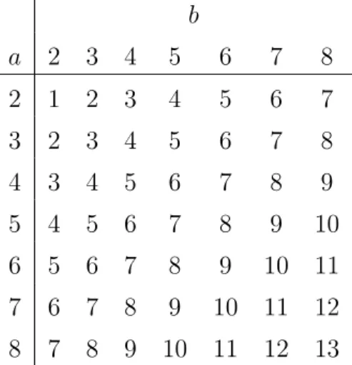
Table 1.1: Estimated Error Degrees of Freedom for a× b Data Using Rank Method.
b
a 2 3 4 5 6 7 8
2 1 2 3 4 5 6 7
3 2 3 4 5 6 7 8
4 3 4 5 6 7 8 9
5 4 5 6 7 8 9 10
6 5 6 7 8 9 10 11
7 6 7 8 9 10 11 12 8 7 8 9 10 11 12 13
Then the orthogonality assumptions add
rank{g˙(α∗, β∗, γ∗)}=dfb
E
degrees of freedom for error whereα∗, β∗, and γ∗satisfy the orthogonality assumptions.
Using numerical differentiation and simulation methods, this idea can be used to find
the error degrees of freedom for the general case of a × b data. Using a − 1 and b−1 degrees of freedom for the main effects and if dfbE represents the estimated error degrees of freedom, then the degrees of freedom assigned to interaction is estimated by
b
dfAB =ab−a−b−dfbE+ 1. We call this method for assigning degrees of freedom the rank method. Table 1.1 gives the error degrees of freedom computed using the rank method for several values of aandb. The rank method typically yieldsdfbE =a+b−3, so when we reference the rank method in following sections, we will be referring to the
Table 1.2: Rank DF and Adjusted Rank DF for 6 × 6 OI Data
Source Rank DF Adjusted Rank DF
FactorA 5 3.71
Factor B 5 3.71
A×B 16 18.58
Error 9 9
The rank method described in this subsection provides degrees of freedom for error
by subtracting degrees of freedom from the traditional (a− 1)× (b −1) degrees of freedom for interaction. Because the orthogonality assumptions put constraints on the
main effects and interactions, it may be inappropriate to provide degrees of freedom
for error merely by subtracting degrees of freedom from interaction. A variation of
the rank method involves rescaling the degrees of freedom for the main effects and
interactions so that the orthogonality constraints impact them both. The degrees of
freedom for error are found in the same way as above, but then define a constantr and let
b
dfA =r(a−1), dfbB =r(b−1), and dfbAB =r(a−1)(b−1).
The constant r is found by forcing the estimated degrees of freedom to sum to ab−1, resulting in r = (ab−1)−1(ab−1−dfb
E). Table 1.2 shows the estimated degrees for
6×6 OI data using the rank method as well as the adjusted rank method (adjustment term r=.743). Using the adjusted rank degrees of freedom results in higher estimated degrees of freedom for interaction and lower estimated degrees of freedom for main
A resampling-based method can also be used to estimate the degrees of freedom
for each source of variation in the orthogonal interactions model. The method involves
adding noise to the data in varying magnitudes and observing the change in the average
sums of squares. We present this method in Chapter 2. The resampling method offers
more reliable estimates for the degrees of freedom, but it requires more computation
than the rank method described in this section.
Partitioning Sums of Squares
After estimating the degrees of freedom for each source of variation, the next step in
using the orthogonal interactions model is partitioning the sums of squares. We borrow
from linear models theory again, using the following definitions of sums of squares
SST = b X j=1 a X i=1
(Yij −Y..)2, (1.22)
SS(A) =b a
X
i=1
ˆ
α2i, SS(B) =a b
X
j=1
ˆ βj2,
SS(AB) = b X j=1 a X i=1 ˆ
γ2ij, and SSE = b X j=1 a X i=1
(Yij −Y..−αiˆ −βjˆ −γijˆ )2.
When fitting the OI model to replicated data, the sums of squares in (1.22) are modified
by summing over the replicates. Using this partitioning of the sum of squares, it can be
shown that the sums of squares are additive, meaning that the total sum of squares is
equal to the sum of the sum of squares for the other sources of variation in the model.
total sum of squares: SST = b X j=1 a X i=1
(Yij −Y..)2
= b X j=1 a X i=1
(Yij −Y..−αiˆ −βjˆ −γijˆ + ˆαi+ ˆβj+ ˆγij)2
= b X j=1 a X i=1
(ˆeij + ˆαi+ ˆβj + ˆγij)2
= b X j=1 a X i=1 n ˆ
e2ij + 2ˆeij(ˆαi+ ˆβj + ˆγij) + (ˆαi+ ˆβj + ˆγij)2o
= b X j=1 a X i=1 n ˆ
e2ij + 2ˆeij(ˆαi+ ˆβj + ˆγij) + ˆα2i + ˆβj2+ ˆγij2 + 2ˆαiβjˆ + 2ˆαiγijˆ + 2 ˆβjγijˆ
o
= SSE + SS(A) + SS(B) + SS(AB)
+2 b X j=1 a X i=1 n ˆ
eij(ˆαi + ˆβj + ˆγij) + 2ˆαiβjˆ + 2ˆαiγijˆ + 2 ˆβjˆγij)o.
From here, we know that:
b X j=1 a X i=1 ˆ αiβjˆ =
b X j=1 ˆ βj a X i=1 ˆ αi ! = 0, b X j=1 a X i=1 ˆ αiˆγij =
a X i=1 ˆ αi b X j=1 ˆ γij ! = 0, and b X j=1 a X i=1 ˆ βjˆγij =
Now the total sum of squares can be written:
SST = SSE + SS(A) + SS(B) + SS(AB) + 2 b X j=1 a X i=1 n ˆ
eij(ˆαi+ ˆβj + ˆγij)o.
Showing that PjPieijˆ (ˆαi + ˆβj + ˆγij) = 0 would be sufficient to prove that the sums of squares are additive. We will do this by showing that
X
j
X
i ˆ
eijαiˆ =X j
X
i ˆ
eijβjˆ =X j
X
i ˆ
eijγijˆ = 0.
Using the results in Appendix A.1,
b X j=1 a X i=1 ˆ
eijαiˆ = tr ˆeTαˆ1Tb
= trn(Y −Y..1a1Tb −αiˆ1 T
b −1aβˆT −γˆ)Tαˆ1Tb
o
= trn(YT −Y..1b1Ta −1bαˆT −βˆ1Ta −ˆγ T
)ˆα1Tb
o
= tr(YTαˆ1T
b −Y..1b|{z}1Taαˆ
0
1bT −1bαˆTαˆ1Tb −βˆ1 T aαˆ
|{z} 0
1Tb −γˆTαˆ
|{z} 0
1Tb)
= tr YTαˆ1Tb −1bαˆTαˆ1Tb
= trnYT(I−PU)Ya1Tb −1bY T
a(I−PU)Ya1Tb
o
= trn1TbYT(I−PU)Ya−1Tb1bY T
a(I−PU)Ya
o
= trn1TbYT(I−PU)Ya−bY T
a(I−PU)Ya
o
Remember that Ya=b−1Y1b−Y..1a, which means that Y1b =b
YTa +Y..1a
. b X j=1 a X i=1 ˆ
eijαiˆ = trnbYTa +Y..1Ta
(I−PU)Ya−bY T
a(I−PU)Ya
o
= trnbYTa(I−PU)Ya−bY T
a(I−PU)Ya
o
, (PU projects onto1a)
= 0.
We use a similar argument to show that PjPieijˆ βjˆ = 0. Using results from Ap-pendix A.1, b X j=1 a X i=1 ˆ
eijβjˆ = trˆeT1aβˆT
= trn(Y −Y..1a1Tb −αiˆ1 T
b −1aβˆT −γˆ)T1aβˆT
o
= trn(YT −Y..1b1Ta −1bαˆT −βˆ1Ta −ˆγ T
)1aβˆT
o
= tr(YT1
aβˆT −aY..βˆT1b
| {z } 0
−1bαˆT1a
| {z } 0
ˆ
βT −βˆ1Ta1aβˆT −γˆT1a
| {z } 0
ˆ βT)
= trYT1aβˆT −βˆ1Ta1aβˆT
= trnYT1aYTb(I−PV)−a(I−PV)YbY
T
b(I−PV) o
= trnYTb(I−PV)YT1a−aY T
b(I−PV)Yb
o
.
Remember that Yb =a−1YT1a−Y..1b and that YT1a =a(Yb+Y..1b). Then,
b X j=1 a X i=1 ˆ
eijβjˆ = trnaYTb(I−PV)(Yb +Y..1b)−aY T
b(I−PV)Yb
o
= trnaYTb(I−PV)Yb−aY T
b(I−PV)Yb
o
, (PV projects onto 1b)
The last step in showing that the sums of squares are additive is to show thatPjPieijˆ γijˆ = 0. Again, using results from Appendix A.1,
b X j=1 a X i=1 ˆ
eijγijˆ = tr ˆeTˆγ
= trY −Y..1a1Tb −αiˆ1 T
b −1aβˆT −γˆ
T
ˆ γ
= trnYT −Y..1b1Ta −1bαˆT −βˆ1Ta −γˆT
ˆ γ
o
= tr(YTγˆ
−Y..1b 1Taˆγ
|{z} 0
−1bαˆTˆγ
|{z} 0
−βˆ1Taγˆ
|{z} 0
−γˆγˆT)
= tr YTˆγ−ˆγTˆγ
= trYT(I−PA)r(I−PB)−(I−PB)rT(I−PA)r(I−PB)
= trYT(I−PA)r(I−PB)−(I−PB)rT(I−PA)r .
Now recall that r=Y −Y..1a1Tb −αˆ1Tb −1aβˆT. Then
b X j=1 a X i=1 ˆ
eijˆγij = tr{YT(I−PA)r(I−PB)
−(Y −Y..−αˆ1Tb −1aβˆT)T(I−PA)r(I−PB)
| {z }
κ
}
Now focusing on tr(κ),
tr(κ) = trn(Y −Y..1a1Tb −αˆ1Tb −1aβˆT)T(I−PA)r(I−PB) o
= trn(YT
−Y..1b1Ta −1bαˆT −βˆ1Ta)(I−PA)r(I−PB) o
= tr{YT(I−PA)r(I−PB)−(Y..1b1Ta −1bαˆT −βˆ1Ta)(I−PA)r(I−PB)
| {z }
=0because PA projects onto1a and ˆα }
= trYT(I−PA)r(I−PB) .
So then:
b
X
j=1
a
X
i=1
ˆ
eijγijˆ = trYT(I−PA)r(I−PB) −tr
YT(I −PA)r(I−PB)
= 0.
Now we have shown that Pbj=1Pai=1eijˆ αiˆ =Pbj=1Pia=1eijˆ βjˆ =Pbj=1Pai=1eijˆ γijˆ = 0, which is sufficient to prove that
SST = SS(A) + SS(B) + SS(AB) + SSE,
where the sums of squares are defined in (1.22).
1.6.2
Inference and Existing Methods
In order to perform inference on the AMMI model, degrees of freedom must be assigned
to each source of variation in the model. Several methods exist for assigning degrees
the degrees of freedom for the main effects are the same as in the additive ANOVA
model. Gauch [2] provides a survey of the different methods of estimating the degrees of
freedom for the interaction terms in the AMMI model. Fora×bdata, the most simple way of assigning degrees of freedom to this model is to assigna+b−1−2mdegrees of freedom to themthPCA axis included in the model. This method of assigning degrees of freedom is called Gollub’s Rule. Cornelius [6] suggests that the Gollub degrees of
freedom lead to high Type I error rates in tests for main effects and interactions.
Other methods for assigning degrees of freedom to the AMMI model involve
sim-ulation. The pure noise method estimates degrees of freedom for each PCA axis for general a×b data, independent of the data of interest. For each of the r simulation replicates, an a×b matrix e is created where eij iid∼ N(0, σ2). If we are interested in
estimating degrees of freedom for the AMMI(m) model, we must fit the main effects
ANOVA model to e, as well as the AMMI(1) through AMMI(m) models. For each simulated data matrix e, sums of squares are calculated for each PCA axis using the following equations:
SS(PCA 1) = SSE(Main Effects ANOVA)−SSE{AMMI(1)} SS(PCA 2) = SSE{AMMI(1)} −SSE{AMMI(2)}
...
SS(PCA m) = SSE{AMMI(m)} −SSE{AMMI(m−1)}.
for each principal component axis are estimated using the following equations:
b
dfj(PCA 1) =
SSj(PCA 1) σ2 b
dfj(PCA 2) =
SSj(PCA 2) σ2
...
b
dfj(PCAm) = SSj(PCAm) σ2 .
Averaging over simulation replicates yields the following estimate for the degrees of
freedom associated with the ith principal component axis:
b
df(PCA i) =r−1 r
X
j=1 b
dfj(PCAi).
The estimated degrees of freedom for error are then obtained by subtraction. For
simplicity, σ2 = 1 is a natural choice for the variance of the generated noise. The pure noise method assumes that there is no signal in the data, which may limit interest in this
method because it does not make use of the data of interest. Another complication with
this method is that it could yield a negative estimate for the error degrees of freedom.
If the degrees of freedom for each PCA axis is overestimated, then the estimated error
degrees of freedom may be negative. The method does not offer an obvious correction if
the estimated error degrees of freedom is negative, but a negative estimate may suggest
that fewer PCA axes should be included in the model.
The pattern plus noise method is similar to the pure noise method, but it makes use of the data of interest. To use this method, first fit the main effects ANOVA model
is generated by adding N(0, σ2
2) noise to the response variable. The AMMI(1) through
AMMI(m) models are fit to each simulated data set. Partitioning the sum of squares
for each PCA axis in the same way as the pure noise method, the degrees of freedom
for the ith PCA axis for thejth simulation replicate is estimated by:
b
dfj(PCA i) = SSj(PCAi) ˆ
σ12+σ22
.
Averaging over the simulation replicates yields the degrees of freedom estimate
b
df(PCAi) = r−1 r
X
j=1 b
dfj(PCA i)
for theith principal component axis in the model. Just as with the pure noise method, the estimated error degrees of freedom are obtained by subtraction, which could
po-tentially yield a negative estimate.
Unlike the AMMI model, assigning degrees of freedom to Tukey’s model is
straight-forward. For a×b data, experimental factors A and B are assigned a−1 and b−1 degrees of freedom respectively. As the name suggests, the multiplicative interaction
parameter for the model is assigned a single degree of freedom.
After fitting the AMMI model or the Tukey one-degree-of-freedom model and
esti-mating degrees of freedom, inference on these models is simple. As in linear models,F ratios are formed to test for main effects and interaction using the error mean square as
axis in the AMMI model can be done using
F = MS(PCA i)
MSE ,
and comparing F to the critical value of the appropriate reference distribution.
1.7
Recognizing Data from the Orthogonal
Inter-actions Model
When working with data from a two-factor experiment, investigators often look at
mean profiles to visualize interactions. When fitting the ANOVA model for example,
parallel mean profiles suggest that interactions should not be included in the model.
We investigated several simulated data sets to see if mean profiles can be used to
determine whether or not the orthogonal interactions model is appropriate for a given
data set. After considering these simulated data sets, we believe that although mean
profiles do provide evidence of interactions, they provide little evidence in determining
if interactions are of the form of the OI model.
A set of main effect and interaction parameters (α,β, andγ1) were created randomly
to satisfy the assumptions of an 8×4 ANOVA model. Then using the reparameteriza-tion described in Secreparameteriza-tion 1.4.1, γ1 was reparameterized to createγ2 so thatα,β, andγ2
satisfy the OI model assumptions. Figure 1.1 displays population mean profiles for the
two different sets of parameters. The means in Figure 1.1(a) come from the orthogonal
interactions model, while the means in Figure 1.1(b) come from a two-factor ANOVA
1 2 3 4 5 6 7 8
6
8
10
12
14
Level of Factor A
Mean Response
(a)
1 2 3 4 5 6 7 8
6
8
10
12
14
Level Of Factor A
Mean Response
(b)
Figure 1.1: Mean Profiles: (a)OI Model(b) ANOVA Model
profile from the OI model can be similar to a mean profile from the ANOVA model.
The similarity in the two profiles suggests that mean profiles are not a useful tool in
determining if the orthogonal interactions model is appropriate for a particular data
set. However, the profiles also suggest that the OI model is capable of modeling ‘real’
data well because predictions from the OI model can be very similar to predictions
from the two-factor ANOVA model with interactions.
When considering the mean profiles in Figure 1.1, it is important to consider how
the means were generated. Because α, β, and γ1 were generated using independent
random normal variates, they essentially satisfy a random effects model. Since the
random effects model provides the motivation for the orthogonal interactions model,
the similarity between the population mean profiles in Figure 1.1 should not be
mean profile for the ANOVA model may look much different than the profile for the
orthogonal interactions model. However, in Section 1.9 we present real data where the
prediction profile from the OI model is very similar to the prediction profile from the
ANOVA with interactions.
Using Biplots to Aid in Model Selection
Biplots are used frequently in determining what type of interactions are appropriate
for a particular data set. See Bradu and Gabriel [9] or Crossa, Cornelius, and Yan [10]
for more information on using the biplot for studying interaction. For unreplicated
two-factor data with a levels of factor A and b levels of factor B, let r be the a×b matrix of residuals from the main effects ANOVA model. Then obtain the singular
value decomposition of r as described in Section 1.5.1, yielding r = UQVT. The matrices Uand V can be represented as
U=
u1, u2, . . . ub
and V=
v1, v2, . . . vb
,
where ui are a×1 eigenvectors andvi are b×1 eigenvectors. Let Y1 denote the a×1
vector of row means ofY and letY2 denote theb×1 vector of column means ofY. In
other words,
Y1,i =b−1
X
j
Yij and Y2,j =a−1
X
i Yij.
The biplot is obtained by plotting u1 versus Y1 and v1 versus Y2 on the same set of
axes.
one-degree-of-freedom form or if they are of the form of the linear-bilinear model. If all of
the points in the biplot lay on a single line, then Tukey’s model is appropriate for the
data. If the points associated with the row effects are linear (or likewise for the column
effects), then the linear-bilinear model is appropriate for the data.
Figure 1.2 shows example biplots for data from Tukey’s model as well as data from a
linear-bilinear model. Tukey’s model is clearly appropriate for the data in Figure 1.2(a)
because all of the points lay on a single line. The biplot in Figure 1.2(b) clearly comes
from a linear-bilinear model because the row effects (represented by circles) are linear
while the column effects (represented by triangles) are not linear.
Similar to the linear-bilinear model, the AMMI model is appropriate for data if
the column effects lay on multiple lines and the row effects also lay on multiple lines
in the biplot. If the number of levels of each experimental factor is small, then the
biplot may not have enough points to aid in deciding on what model is appropriate.
For three levels of each experimental factor, the biplot would only consist of six points,
which would not be sufficient for drawing any conclusions about the nature of the
interactions.
After inspecting many biplots of data generated from the orthogonal interactions
model, we do not find a feature unique to biplots of data from the OI model. This is
due to the fact that interactions from the OI model are not multiplicative in nature as
they are in the Tukey, linear-bilinear, and AMMI models. Because the biplot uses the
singular value decomposition of the residuals, it is effective in detecting multiplicative
interactions. So looking at a biplot does not immediately allow investigators to
deter-mine whether or not the OI model is appropriate for data. However, if the biplot does
−1.0 −0.5 0.0 0.5 1.0
−8
−6
−4
−2
0
2
4
First Eigenvector
Mean Response
Row Effect Column Effect
(a)
−1.0 −0.5 0.0 0.5 1.0
−8
−6
−4
−2
0
2
4
First Eigenvector
Mean Response
Row Effect Column Effect
are appropriate for the data, then the OI model is a possible choice.
1.8
Testing the Orthogonality Assumptions
For replicated data, fitting the orthogonal interactions model instead of the full ANOVA
model may result in a more efficient estimate of the error variance. Although the
orthogonal interactions model is not a linear model, it is in fact nested within the
full two-factor ANOVA model with interactions. The model is nested within the full
ANOVA model in the sense that when both models are fit to data, the error sum
of squares for the OI model will always be greater than or equal to the error sum
of squares for the full ANOVA model. If the OI and ANOVA models are written
E(Y) = Xθ1 and E(Y) = Xθ2 respectively, let Θ1 represent all possible solutions for
θ1 and let Θ2 represent all possible solutions for θ2. We know that Θ1 ⊂ Θ2 because
the OI model is a special case of the full ANOVA model. Since Θ1 ⊂ Θ2, we know
that the error sum of squares for the OI model is greater than or equal to the error
sum of squares for the ANOVA model, and therefore the OI model is nested within the
ANOVA model. Because of this nesting, the likelihood ratio test is the natural choice
for testing the orthogonality assumptions for replicated data. The remainder of this
section discusses using the likelihood ratio test for testing the appropriateness of the
orthogonality assumptions.
We are interested in testing the hypothesis
which is equivalent to
H0 : OI model sufficient vs. H1 : Full ANOVA necessary. (1.23)
The hypothesis written in (1.23) is a full-versus-reduced model comparison where the
full model does not require the model parameters to satisfy the orthogonality
con-straints. If l0 represents the log-likelihood of the reduced model andl1 represents the
log-likelihood of the full model, then
W = 2(l1 −l0) (1.24)
is the usual likelihood ratio test statistic. The test statistic in (1.24) is compared to the
χ2d distribution where d is equal to the difference in the number of parameters in the two models (see Section 1.6.1 for estimating degrees of freedom for the OI model). If
the rank degrees of freedom are used for the OI model, then the likelihood ratio test is
compared to aχ2
a+b−3 distribution where a andb are the levels of experimental factors
A and B respectively.
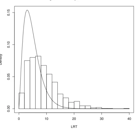
The problem with the likelihood ratio test statistic defined in (1.24) is that the
statistic converges to the χ2 distribution as c, the number of replicates per factor-level combination, tends to infinity. For smallc, the Type I error rate can be very high as we show later. Real data typically do not feature a large enough number of replicates to
avoid this problem of inflated Type I error rate, so the test statistic must be adjusted
to correct this problem. Bartlett ([11] and [12]) and Lawley [13] provide the basis
test statistic in order to improve the quality of the χ2 approximation for small sample
sizes (small c). More recent work by Barndorff-Nielsen and Cox [14] and Cordeiro [15] provide more justification for the Bartlett correction and extend the correction to
nonlinear models. Simulations by Cordeiro [15] show that the Bartlett correction can
reduce the Type I error rate from 30% to a more acceptable 8% in nonlinear models.
Since the OI model is nonlinear, we expect that the Bartlett correction can also reduce
the Type I error rate for the likelihood ratio test of (1.23). We do not provide a
general form for the Bartlett correction to the test statistic in (1.24) though it might
be possible with extensive algebraic manipulations. In the following subsections we
provide simulation-based corrections to the likelihood ratio test in the spirit of the
Bartlett correction.
1.8.1
A Bootstrap Corrected Likelihood Ratio Test
Suppose that investigators are interested in comparing two models by testing the
hy-pothesis
H0 : Model I sufficient vs. H1 : Model II necessary,
where Model I is nested within Model II and there are d more parameters in Model II than in Model I. Then the likelihood ratio statistic W as defined in (1.24) converges in distribution toχ2
dunder the null hypothesis. But for small sample sizes, E(W |H0)6=d
in general. The idea behind the Bartlett correction is to find a parameter k such that E(kW |H0) =d, even for small sample sizes. Finding a general form for the estimator of