Agrometeorology |
Article
methods in four agroecological regions in Colombia
Daniel Rodríguez Caicedo(1*); Jose Miguel Cotes Torres(2); José Ricardo Cure(1)(1) Universidad Militar Nueva Granada, Facultad de Ciencias Básicas, Cra. 11#101-80 Bogotá, Colombia.
(2)Universidad Nacional de Colombia, Departamento de Ciencias Agropecuarias, Calle 59a#63-20, Medellín, Colombia.
(*) Corresponding author: [email protected]
Received: Sept. 20, 2011; Accepted: Mar. 8, 2012
Abstract
Eight methods were used to estimate degree-days in four Colombian localities. Four methods have been previously proposed in literature: Simple Sine, Double Sine, Simple Triangle, and Double Triangle methods. The other four methods are proposed in this research: Simple Logistic, Double Logistic, Simple Normal, and Double Normal. The estimation of the degree-days through hourly temperature values was used as thereference standardmethod, and the four localities from where the tem-perature values were taken were the municipalities of Cajicá (Cundinamarca), Santa Elena (Antioquia), Carepa (Urabá Antio-queño), and Ciudad Bolivar (Zona cafetera Antioqueña). Degree-days obtained by all methods under study were compared through linear regression to those obtained by the reference standardmethod. There were differences in the correlation of
each method to the reference when compared within each region and among regions. The Simple Logistic and Double Lo-gistic methods showed the best performance with acceptable R2 values and considerably lower bias than the other methods.
The poorest fit was found in Cajicá, where the average R2 was 0.571. For the regions of Santa Elena and Carepa, the average
R2 was 0.756 and 0.733. The best fit was found in Ciudad Bolivar, with an average R2 of 0.826. Key words: degree-days, thermal time, temperature threshold, statistical modeling.
Comparação de oito métodos para calcular graus-dia em quatro regiões agroecológicas
Resumo
Estimativas de graus-dia foram obtidas pelos métodos de seno simples e duplo, triangulo simples e duplo, as quais são am-plamente utilizadas. Quatro novos métodos foram propostos e avaliados nesta pesquisa: logística simples e dupla, normal simples e dupla, baseadas em regressão logística e distribuição normal. Registros horários de temperatura obtidos em Cajicá (Cundinamarca), Santa Elena (Antioquia), Carepa (Urabá Antioqueño) e Ciudad Bolivar (Região tradicional da cultura do café) foram utilizados para obter estimativas da soma térmica com maior precisão sendo, portanto, considerada como a referên-cia para comparação utilizando regressão linear. Foram constatadas diferenças entre o ajuste dos métodos dentro de cada
região e entre regiões. Foram observados os maiores coeficientes de determinação (R2), nos métodos de logística simples
e logística dupla. O menor coeficiente de determinação, de 0,571, foi obtido em Cajicá enquanto nas regiões de Medellín e
Carepa, o R2 foi de 0,756 e 0,733 respectivamente. O melhor ajuste foi obtido em Ciudad Bolivar, com um R2 igual a 0,826. Palavras-chave: graus-dia, tempo térmico, temperatura basal, modelagem estatística.
1. INTRODUCTION
The concept of degree-days has been widely used in agriculture, especially to quantify and predict phe-nological events, because it is more accurate than us-ing chronological time or the predictions of events according to the season of the year (McMaster and Wilhelm, 1997). Degree-days have been used in phenological analysis applied to different kind of crops, both in temperate zones (Narwal et al., 1986; Allen and O’brien, 1986; Undersander and Christiansen, 1986; Jones et al., 1991; Sharratt et al., 1989; Spencer et al., 2000; Spencer and Ksander, 2006) and in tropical zones
as well (Lemos et al., 1997; McBeth et al., 2001; Bell and Wright, 1998; Jullien et al., 2008; Guan et al., 2009). Degree-days also have been used in in-sect phenology studies (Tokeshi, 1985; Lindblad and Sigvald, 1996; Hart et al., 1997; Broufas and Koveos, 2000; Milonas et al., 2001; Olsen, 2003; Hirata and Higashi, 2008; Kumral et al., 2008; Naves and Sousa, 2009; Nietschke et al., 2007; Elliot et al., 2009).
The basic equation for the calculation of degree-days is (McMaster and Wilhelm, 1997):
MTT T
T
DD= + −
2
min max
Where DD are the degree-days, Tmax and Tmin are the daily maximum and minimum temperatures, respectively, and MTT is the minimum temperature threshold. In [1] it is assumed that if [(Tmax + Tmin)/2]> MTT, then DD>0, but if [(Tmax + Tmin)/2]< MTT, there is no accumulation
of thermal time and DD = 0. Equation [1], however, can underestimate degree-days when temperatures fluctuate above and below the minimum threshold. The reason for this underestimation is that organisms grow and develop during the periods of the day when the temperature is above the minimum temperature threshold, even if at the end of the day the daily average temperature is lower than that minimum threshold. Some methods based on the daily temperature fluctuation pattern have been pro-posed in order to correct this problem. The most widely used of these methods, from the simplest to the more complex, are: Simple Triangle, Double Triangle, Simple Sine and Double Sine. These methods assume that the minimum daily temperature is reached at midnight, while the maximum daily temperature is reached at noon; these methods also allow consideration of a maximum tem-perature threshold above which the organism of interest doesn’t progress. There is scant information about com-parisons among the different methods. Roltsch et al. (1999) evaluated the above-mentioned four methods in California climates. They found that compared to the Simple Sine and Simple Triangle methods, the Double Sine and Double Triangle methods did not offer a signifi-cant improvement in the estimation of degree-days. The same authors found differences in the performances of the methods when used in different regions; these results indicate that a method considered functional in a region might not be the best one for other regions, and there-fore it is recommended to evaluate different methods and determine which one is superior for a specific region. To date, this research is the first in Colombia addressing that goal. The purpose of this research was to evaluate four previously published methods to estimate degree-days in four Colombian regions, and compare them to four new methods proposed in this study.
2. MATERIAL AND METHODS
All the estimations in this research were done us-ing hourly temperature data from four weather stations: (1) the weather station at Rio Grande experimental farm in Cajicá, Cundinamarca, located at an altitude of 2558 m. with an annual average temperature of 14 °C (57.2 °F), classified as a Lower Montane dry forest life zone according to the Holdridge life zone system, and from where 364 days of data were used; (2) the weather station at Paisandú experimental farm in Santa Elena, Antioquia, located at 2500 m., with an annual average temperature of 14 °C (57.2 °F) and classified as a Lower Montane
humid forest life zone; the data analyzed from this sta-tion included 304 days of hourly temperatures; (3) the Augura weather station in Carepa, Antioquia, located at an altitude of 40 m., with an annual average temperature of 25 °C (77 °F), classified as a Tropical humid forest life zone, and from where 181 days of data were analyzed; (4) the weather station in Ciudad Bolivar, Antioquia, located at 1429 m., with an average annual temperature of 22 °C (71.6 °F), and classified as a Premontane humid forest life zone; the data used from this station included 128 days of hourly temperatures.
The data were classified according to the six pos-sible situations that can occur when comparing daily temperature curves with the temperature thresholds: (1) the minimum temperature is higher than the minimum threshold and the maximum temperature is higher than the maximum threshold; (2) the minimum temperature is lower than the minimum threshold and the maximum temperature is higher than the maximum threshold; (3) both maximum and minimum temperatures are within thresholds; (4) the minimum temperature is lower than the minimum threshold and the maximum temperature is lower than the maximum threshold; (5) both minimum and maximum temperatures are higher than the maxi-mum temperature threshold, and (6) both maximaxi-mum and minimum temperatures are lower than the minimum threshold. The methods previously published, and the new methods proposed here allow making adjustments to include the effect of each of the six described situations. In order to evaluate the six methods within each location, both the minimum and maximum temperature thresh-olds were estimated as the average of the minimum and maximum daily temperatures for the evaluation period, respectively. In this way, an approximately equal number of data was assigned to each method.
Two approaches have been proposed for the cases when the maximum daily temperature is higher than the maximum temperature threshold (Roltsch, 1999): (1) the Vertical Cutoff method considers that there is no accumulation of thermal time when the maximum tem-perature rises above the maximum temtem-perature threshold; (2) the Horizontal Cutoff method assumes that thermal time keeps accumulating when temperature is above the maximum temperature threshold, but the difference between the maximum temperature and the maximum threshold doesn’t contribute to the accumulated thermal time. The latest approach was used in this research.
Logistic, Double Logistic, Simple Normal, and Double Normal. The first two methods assume that temperatures fluctuate during the day according to a logistic model and the last two methods assume that temperatures fluctuate during the day according to a normal distribution. All the new methods also allow for appropriate adjustments ac-cording to the six different situations that can occur when comparing the daily temperature curve with the mini-mum and maximini-mum thresholds.
Symmetric Methods
One of the approaches to degree-day modeling is to assume that the temperature curve is symmetric around the maximum temperature. The following methods use this approach.
Simple Triangle (Lindsey and Neuman, 1956): In this method, a straight line is drawn from the minimum temperature, assumed at 00:00 hours, to the maximum temperature, assumed at 12:00 hours, and from there, to complete the two sides of a triangle, another straight line is drawn to the next day’s minimum temperature, which is assumed to be the same minimum tempera-ture used for the first half of the day (Figure 1a). The accumulated degree-days are estimated as the area un-der the triangle and between the thresholds. As can be seen from the figure, temperature fluctuations do not necessarily behave according to the assumptions of the method and for the first two days the method overestimates the degree-days during the morning and underestimates them in the afternoon. The third day, the method overestimates the degree-days both in the morning and in the afternoon.
Simple Sine (Baskerville and Emin, 1969): As can be seen from figure 1c, the changes in temperature are closer to a soft curve than to a straight line as assumed in the Simple Triangle method. By assuming that the varia-tion of daily temperatures follows a sine funcvaria-tion closely, the Simple Sine method offers a better approximation of the curvilinear behavior of the temperature. As in the previous method, the minimum daily temperature is the same for both halves of the day and degree-days are esti-mated as the area under the sine curve and between the thresholds.
Simple Logistic (proposed): This method is based on the logistic model and assumes that in each half of the day the temperature fluctuates according to the lo-gistic equation (Fox, 2002). As in the Simple Sine and Simple Triangle methods, it is assumed that tempera-tures are symmetric around the maximum temperature (Figure 1e). In [2] T is the temperature expressed as a function of the hour of the day, t . The parameter β
1 is the
day’s maximum temperature, β2indicates the temperature
at 00:00, and β3controls the rate of temperature change.
t
β
+
e
+
β
=
T
β2 3 1
1
[2]Assuming as in the previous models that the mini-mum temperature, Tmin, is reached at 00:00 hours, the parameter β2 can be obtained as follows:
−
1
log
min 1 2T
β
=
β
eSince different models assume that the minimum temperature occurs at 00:00 hours and the maximum at 12:00 hours, it was considered reasonable to assume that (Tmax + Tmin)/2 occurs at 6:00 hours; this allows a third temperature value that can be used to estimate β3 and
complete the parameters of the model.
6 1 log 2 min max max 3 − − β T + T T = β e
Degree-days are estimated by solving the integral of model [2] between 0 and 12. Since the integration is solved considering time as an independent variable ex-pressed in hours, the result of the integration is an estima-tion of degree-hours, therefore this value has to be divided by 24 to become degree-days, and then multiplied by 2 because it is assumed that the thermal accumulation is the same for the two halves of the day.
MTT β ) + β + t (e β t β = DD 2 β − − ∗ 24 1 ln 2 12 0 3 3 1 1
The necessary adjustments to the six situations previously described in the introduction can be im-plemented by using the inverse function of [2] to find the hour of the day in which a specific threshold is reached, and limiting the integral to the appropriate range of hours.
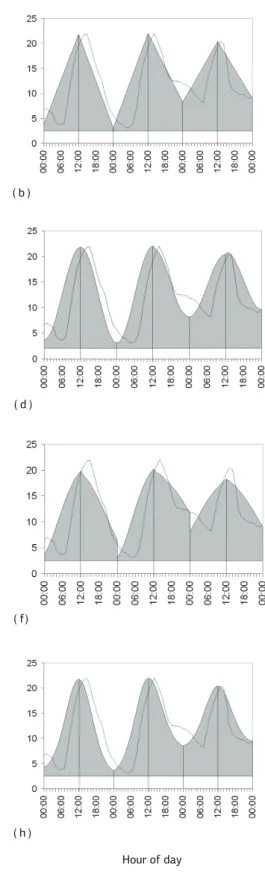
Figure 1. Graphic comparison of the evaluated degree-day estimation methods. The X-axis represents the hours of the day during a period of three days. The Y-axis represents the temperatures during the day. The blue line shows the observed temperatures during three days in Cajicá, Cundinamarca. The gray area represents the degree-days accumulated by each of the following methods: (a) Simple Triangle, (b) Double Triangle, (c) Simple Sine, (d) Double Sine, (e) Simple Logistic, (f) Double Logistic, (g) Simple Normal, and (h) Double Normal.
T
e
m
p
e
ra
tu
re
( a )
T
e
m
p
e
ra
tu
re
( b )
( c ) ( d )
( e )
( f)
( g ) ( h )
time when the minimum temperature is reached, and is equal to Tmax – Tmin at 12:00, the time when the maxi-mum temperature is reached (Figure 1g).
K e
π =
T
T(t) [(t ) ] ×
⋅ ⋅
− −0.5⋅ −12/4.5 2
min 4.5 2 1 [3] where − ⋅ ⋅ − ⋅
−0.5 1212 /4.5 2 min
max 2 4.5
] ) [( e π ) T (T =
K [4]
simplifying [3] and [4] :
) T (T e = T
T(t) [(t ) ]
min max 2 4.5 / 12 0.5 min − − − ⋅ − [5]
Since the integral of a normal density function is equal to 1, the integral of [5] is equal to K. Therefore, to obtain the area under the curve of the expression [5], the probabilities of a standard normal distribution can be used and multiplied by the mentioned value K. To calcu-late the probabilities, 00:00 and 12:00 are transformed into values of a standard normal distribution (z=-2.67 and z=0.00, respectively), and the degree-days can be ob-tained as indicated in (6):
MTT e π ) T (T )] < p(z ) < [p(z + T = DD ] ) [( − ∗ ⋅ ⋅ − ∗ − − ∗ − ⋅
−0.5 12 12 /4.5 2 min max min 24 4.5 2 2.67 0.0 2 [6]
It is divided by 24 and multiplied by 2 for the same reasons already explained in the discussion of the Simple Logistic method. The necessary adjustments to the six situations previously described in this section can be implemented by using the inverse function of the normal density function to determine the hour in which a specific threshold is reached, which allows lim-iting the calculation of probabilities to the appropriate range of hours.
Asymmetric Methods
Daily temperatures do not necessarily fluctu-ate symmetrically around the maximum temperature, which could lead the previous methods to inaccu-rate degree-day estimations. The following so-called “double” methods attempt to correct this situation by
considering different minimum temperatures for each half of the day. In these methods, the minimum tem-perature for the first half of the day is the actual mini-mum temperature of the day while the minimini-mum tem-perature for the second half of the day is the minimum temperature of the following day. For these methods, the necessary adjustments to the six situations men-tioned above are done for each half of the day.
Double Triangle (Sevacherian et al., 1977): The degree-days for the day are calculated as the sum of the degree-days for the two half-days, which are esti-mated as the area within the triangle and between the thresholds (Figure 1b).
Double Sine (Allen, 1976): This method fits a dif-ferent sine curve for each half of the day using the appro-priate minimum and maximum temperatures (Figure 1d). The degree-days are calculated as the sum of the areas un-der the curves and between the thresholds (McMaster and Wilhelm, 1997).
Double Logistic (proposed): The procedure is similar to that described for the Simple Logistic method, but in this case it is necessary to estimate the parameters and to integrate separately for each half of the day. The param-eter β1 is the same for both halves of the day, but for each
half of the day, β2 andβ3must be estimated using the
appropriate Tmin value (Figure 1f).
Double Normal (proposed): The procedure is also similar to that described for the Simple Normal method, but the value of K has to be estimated for each half of the day based on the appropriate minimum temperature. (Figure 1h).
Comparison of Methods
The estimation of degree-days through the area un-der the curve of hourly temperatures was consiun-dered the reference standard method because this procedure is more accurate than the methods that use minimum and maximum temperatures. The integration was solved using the midpoint rule.
In order to evaluate the eight methods under study, linear regression models were estimated for each combi-nation of method and locality. The dependent variable was the degree-days estimated by each of the methods and the independent variable was the degree-days cal-culated with the reference standard method. Fitting performance of the models was evaluated through the coefficient of determination (R2), and the bias of the
RESULTS AND DISCUSSION
Cajicá, Cundinamarca
The intercepts for the Simple Triangle, Double Sine, and Simple Normal methods were statistically significant according to Student’s t-test. From the new methods, only the Double Normal had a statistically significant intercept. The four methods previously pro-posed in literature showed values of bias around 18%, a value close to that of the Double Normal method
which had the highest bias (18.43%). The Simple Logistic and Double Logistic methods presented sig-nificantly lower bias, indicating a better estimation of the accumulated degree-days. Considering the R2
alone, the best fit was shown by the Simple Triangle and Simple Sine methods, followed by the Simple Logistic method. The two first methods, however, had high bias and therefore the Simple Logistic method is a better option for the estimation of accumulated de-gree-days in this region. The Double Normal method had the highest bias and the lowest R2, therefore its use
is not recommended for this locality.
Table 1. Results for the eight evaluated methods in four localities.
Method β0
ˆ β
1
ˆ
R2 Total GD¥ Bias
Cajicá
Simple Triangle 0.05615** 1.1662** 0.6245 1767.630 17.98
Simple Sine 0.4442 1.0701** 0.6351 1764.990 17.81
Double Triangle 0.3812 1.0876** 0.5588 1768.300 18.03
Double Sine 0.7426** 0.9979** 0.5688 1765.470 17.84
Simple Logistic -0.3015 1.1875** 0.6129 1669.384 11.43
Simple Normal -1.4140** 1.4735** 0.5291 1692.939 13.00
Double Logistic 0.03695 1.10578** 0.5446 1670.084 11.47
Double Normal 0.5365 1.3146** 0.4954 1774.264 18.43
Ref. Standard 1498.161
Santa Elena
Simple Triangle 0.4095** 1.0224** 0.7809 1080.520 15.56
Simple Sine 0.6651** 0.9341** 0.7862 1075.628 15.04
Double Triangle 0.5561** 0.9753** 0.7783 1080.996 15.61
Double Sine 0.8028** 0.8897** 0.7749 1075.971 15.07
Simple Logistic 0.1102 1.0498** 0.7693 1015.157 8.57
Simple Normal -0.1858 1.1933** 0.6681 1059.475 13.31
Double Logistic 0.2675 0.9993** 0.7723 1015.688 8.62
Double Normal 0.0862 1.1373** 0.7219 1089.645 16.53
Ref. Standard 935.019
Carepa
Simple Triangle 0.2855** 0.9884** 0.7565 373.550 14.71
Simple Sine 0.45602 0.89081** 0.7655 372.629 14.43
Double Triangle 0.3539** 0.9506** 0.7560 373.611 14.73
Double Sine 0.5605** 0.9181** 0.6262 400.447 22.97
Simple Logistic 0.0287 1.0554** 0.7413 348.866 7.13
Simple Normal -0.2287 1.2594** 0.7324 368.739 13.23
Double Logistic 0.10379 1.0139** 0.7483 348.9689 7.16
Double Normal -0.0619 1.1929** 0.7408 377.2591 15.85
Ref. Standard 325.647
Ciudad Bolívar
Simple Triangle 1.6987** 0.8798** 0.8909 747.189 24.10
Simple Sine 1.8946** 0.8908** 0.6908 786.122 30.57
Double Triangle 1.7353** 0.8692** 0.8690 745.4369 23.81
Double Sine 1.9452** 0.8899** 0.6923 784.8356 30.35
Simple Logistic 1.2584** 0.8967** 0.8889 700.9998 16.43
Simple Normal 1.0823** 0.9873** 0.8540 732.9957 21.74
Double Logistic 1.2948** 0.8859** 0.8714 699.1368 16.12
Double Normal 1.0870** 0.9988** 0.8517 740.5252 22.99
Ref. Standard 602.089
Santa Elena, Antioquia
All the models presented higher R2 values, and
there-fore better fit, in this region than in Cajicá, (Table 1). The intercepts were statistically significant for all previ-ously proposed methods, while the intercepts for all the new methods were not significant. The four previously proposed methods showed the highest R2 values, but also
high values of bias close to 15%. The Simple Normal and Double Normal methods also had high bias. Alternatively, the Simple Logistic and Double Logistic methods showed a much lower bias close to 8.0% and R2 values of 0.76
and 0.74, respectively, values that are very close to those obtained by the previously proposed methods. According to these results, the Simple Logistic and Double Logistic methods presented the best performance in the Santa Elena region. The Double Normal method presented the highest bias with one of the lowest R2 values,
consequent-ly its use is not recommended in this region.
Carepa, Antioquia
From all the evaluated methods, only the Simple Triangle, Double Triangle, and Double Sine methods had models with statistically significant intercepts. The pre-viously published methods showed biases ranging from 14% to almost 23%, while the proposed methods, with the exception of the Double Normal, presented lower bi-ases. The Simple Logistic and Double Logistic methods had biases of 7.13% and 7.16%, respectively, which are practically half of those obtained with the previously pro-posed methods. The Simple Logistic and Double Logistic methods also had R2 values close to 0.74, which can be
considered appropriate compared to those obtained by the other methods. Even though the Double Normal method showed a better R2 value than in the other
re-gions, it is not recommended because it has a bias of 15%, which doesn’t represent an improvement over the previ-ously proposed methods.
Ciudad Bolívar, Antioquia
The R2 values tended to be higher in this locality. A
noticeable exception occurred with the Simple Sine and Double Sine methods, whose models had coefficients of determination that indicate a particularly poor fit. Bias values were also higher in this locality for all the methods. For the previously proposed methods, the bias ranged from 24% to 30% while the new methods had biases between 16% and 23%, with the highest value being that of the Double Normal method. As in the pre-vious localities, the Simple Logistic and Double Logistic methods had the lowest biases with values close to 16%
and acceptable R2 values that allow recommending these
methods for this locality.
The differences among methods were evident and consistent throughout the localities, making it easier to select the best methods. The previously published meth-ods presented acceptable coefficients of determination, but they are not recommended because they showed a tendency to have higher biases than the new methods in all the environments. In many cases the models of the new methods didn’t have statistically significant inter-cepts, which is a desirable property that indicates that those methods would estimate a degree-day value close to zero when the reference standard method actually cal-culates a degree-day value of zero. The Double Normal method had a poor performance and therefore is not rec-ommended. The Simple Logistic and Double Logistic methods had acceptable coefficients of determination along with noticeably lower biases than the other meth-ods. Given that this result was consistent in the four dif-ferent agroecological localities, these two methods can be recommended to be used in Colombia.
There were differences in the performance of the methods among localities, which is consistent with the results found by Roltsch et al. (1999), who found that using the Simple Triangle method, the percent-age error in degree-day estimation in the Intermediate Valley of California was much higher than in the Interior Valley. In this research the best goodness of fit was observed in Ciudad Bolivar, where the average co-efficient of determination was 0.825. Santa Elena and Carepa had intermediate R2 values, 0.753 and 0.733
through the bias, were noticeably lower and none of the methods had a bias higher than 31%. Even though higher variations could be found if the evaluations were done monthly, they wouldn’t be as big as the variations observed in regions with seasons.
In this discussion, the bias was considered as the param-eter of higher importance to evaluate the goodness of fit of the models because biased accumulations of thermal time lead to inaccurate predictions of the phenological events. If the estimated degree-day accumulation is higher than the real one, the chronological time required for the phenologi-cal event will be lower than the real and vice versa, and this could lead to very variable results in terms of population dynamics (Bryant et al. 1998). Finally, it is important to take into account that even though factors like diet in the case of insects or soil fertility and humidity in the case of plants can affect development time, their effect is difficult to measure and relatively small when compared to the ef-fect of temperature, and therefore degree-day estimation re-mains an important tool in the prediction of phenological events both in plants and insects (Herms, 2007).
4. CONCLUSION
The evaluated methods showed differences in their performance that made possible the selection of the Simple Logistic and Double Logistic methods as the best options for degree-day estimation. Since this result was consis-tent in all the localities, it is assumed that both methods can be used under different environmental conditions in the Colombian tropics. The Simple Normal and Double Normal methods are not recommendable because their models showed poor fit and high bias.
REFERENCES
ALLEN, J.C. A modified sine wave method for calculating degree days. Environmental Entomology, v.5, p.388-396, 1976.
ALLEN, E.J.; O’BRIEN, P.J. The practical significance of accumulated day degrees as a measure of physiological age of seed potato tubers. Field Crops Research, v.14, p.141-151, 1986.
BASKERVILLE, G.L.; EMIN, P. Rapid Estimation of heat accumulation from maximum and minimum temperatures. Ecology, v.50, p.514-517, 1969.
BELL, M.J.; WRIGTH, G.C. Groundnut growth and development in contrasting environments. 2. Heat unit accumulation and photothermal effects on harvest index. Experimental Agriculture, v.34, p.113-124, 1998.
BROUFAS, G.D.; KOVEOS, D.S. Threshold temperature for post-diapause development and degree-days to hatching of winter eggs of the European red mite. (Acari: Tetranychidae) in Northern Greece. Environmental Entomology, v.24, p.703-713, 2000.
BRYANT, S.R.; BALE, J.S.; THOMAS, C.D. Modification of the Triangle method of degree-day accumulation to allow for behavioral thermoregulation in insects. Journal of Applied Ecology, v.35, p.921-927, 1998.
ELLIOT, R.H.; MANN, L.; OLFERT, O. Calendar and degree day requirements for emergence of adult wheat midge, Sitodiplosis mosellana (Géhin) (Diptera:Cecidomyiidae) in Saskatchewan, Canada. Crop Protection, v.28, p.588-594, 2009.
FOX, J. Nonlinear regression and nonlinear least-squares. Available at: http://cran.r-project.org/doc/contrib/Fox-Companion/appendix-nonlinear-regression.pdf. 2002. Accessed 27th. Nov. 2009.
GUAN, B.T.; CHUNG, C.H.; LIN, S.T.; SHEN, C.W. Quantifying height growth and monthly growing degree days relationship of plantation Taiwan spruce. Forest Ecology and Management, v.257, p.2270-2276, 2009.
HART, A.J.; BALE, J.S.; FENLON, J.S. Developmental threshold, day-degree requirements and Voltinism of the aphid predator.
Epysirphus balteatus (Diptera: Syrphidae). Annals of Applied Biology, v.130, p.427-437, 1997.
HERMS, D.A. Using degree-days and plant phenology to predict pest activity. In: IPM of Midwest landscapes: tactics and tools for IPM. The Ohio State University 2007. Available from: http:// www.entomology.umn.edu/cues/Web/049DegreeDays.pdf. Accessed in: Nov., 29 2009.
HIRATA, M.; HIGASHI, S. Degree-day accumulation controlling allopatric and sympatric variations in the sociality of sweat bees
Lasioglossum (Evylaeus) baleicum (Hymenoptera:Halictidae). Behavioral Ecology and Sociobiology, v.62, p.1239-1247, 2008.
JONES, E.A.; REED, D.D.; CATTELINO, P.J.; MROZ, G.D. Seasonal shoot growth of planted red pine predicted from air temperature degree days and soil water potential. Forest Ecology and Management, v.46, p. 201-214, 1991.
JULLIEN, A.; CHILLET, M.; MALÉZIEUX, E. Pre-harvest growth and development, measured as accumulated degree-days, determine the post-harvest green life of banana fruit. Journal of Horticultural Science and Biotechnology, v.83, p.506-512, 2008.
KUMRAL, N.A.; KOVANCI, B.; AKBUDAK, B. Using degree-day accumulation and host phenology for predicting larval emergence patterns of the olive psyllid, Euphyllura Phyllireae. Journal of Pest Science, v.81, p.63-69, 2008.
LEMOS, J.P.; VILLA, N.A.; SILVERIA, H. A model including photoperiod in degree days for estimating Hevea bud growth. International Journal of Biometeorology v.41, p.1-4, 1997.
LINDBLAD, M.; SIGVALD, R. A degree-day model for regional prediction of first occurrence of fruit flies on oats in Sweden. Crop Protection, v.15, p.559-565, 1996.
LINDSEY, A.A.; NEWMAN, J.E. Use of Official Weather Data in Spring Time: Temperature Analysis of an Indiana Phenological Record. Ecology v.37, p.812-823,1956.
Impact of heating degree-day accumulation during Bermuda Grass hay storage on nutrient utilization by lambs. Journal of Animal Science, v.79, p.2698-2703, 2001.
MCMASTER, G.S.; WILHELM, W.W. Growing degree-days: one equation, two interpretations. Agricultural and Forest Meteorology, v.87, p.291-300, 1997.
MILONAS, P.G.; SAVAPOULOU-SOULTANI, M.; STAVRIDIS, D.G. Day-degree models for predicting the generation time and flight activity of local populations of Lobesia botrana (Den & Schiff) (Lep.,Tortricidae) in Greece. Journal of Applied Entomology, v.125, p.515-518, 2001.
NARWAL, S.S.; POONIA, S.; SINGH, G.; MALIK, D.S. Influence of sowing dates on the growing degree days and phenology of winter maize (Zea mays L.). Agricultural and Forest Meteorology, v.38, p.47-57, 1986.
NAVES, P.; SOUSA, E. Threshold temperatures and degree-day estimates for development of post-dormancy larvae of Monochamus Galloprovincialis (Coleoptera:Cerambicidae). Journal of Pest Science, v.82, p.1-6, 2009.
NIETSCHKE, B.; MAGAREY, R.D.; BORCHERT, D.M.; CALVIN, D.D.; JONES, E. A developmental database to support insect phenology models. Crop Protection, v.26, p.1444-1448, 2007.
OLSEN, A.; BALE, J.S.; LEADBEATER, B.S.C.; CALLOW, M.E.; HOLDEN J.B. Developmental thresholds and day-degree requirements of Paratanytarsus grimmii and Corynoneura scutellata (Diptera: Chironomidae): two midges associated with potable water treatment. Physiological Entomology, v.28, p.315-322, 2003.
ROLTSCH, W.J.; ZALOM, F.G.; STRAWN, A.J.; STRAND, J.F.; PITCAIRN, M.J. Evaluation of several degree-day estimation methods in California climates. International Journal of Biometeorology, v.42, p.169-176, 1999.
SAMSON, P.R. Interpolating temperatures for simulation of the developmental progress of Pieris rapae (L.) (Lepidoptera:Pieridae). Journal of the Australian Entomological Society, v.23, p.127-131, 1984.
SEVACHERIAN, V.; STERN, V.M.; MUELLER, A.J. Heat accumulation for timing Lygus control measures in a safflower-cotton complex. Journal of Economic Entomology, v.70, p.399-402, 1977.
SHARRATT, B.S.; SHEAFFER, C.C.; BAKER, D.G. Base temperature for the application of the growing-degree-day model to field-grown alfalfa. Field Crops Research, v.21, p.95-102, 1989.
SPENCER, D.F.; KSANDER, G.G.; MADSEN, J.D.; OWENS, C.S. Emergence of vegetative propagules of Potamogeton nodosus,
Potamogeton pectinatus, Vallisneria americana, and Hydrilla verticillata based on accumulated degree-days. Aquatic Botany, v.67, p.237-249, 2000.
SPENCER, D.F.; KSANDER, G.G. Estimating Arundo donax
ramet recruitment using degree-day based equations. Aquatic Botany, v.85, p.282-288, 2006.
TOKESHI, M. Life cycle and production of the burrowing mayfly,
Ephemera danica: A new method for estimating degree-days required for growth. Journal of Animal Ecology, v.54, p.919-930, 1985.