João Filipe Pereira Domingues Alho
Licenciado em Ciências da Engenharia FísicaDevelopment of didactic physics experiments
using a miniaturized wireless acquisition board
Dissertação para obtenção do Grau de Mestre em
Engenharia Física
Orientador: Grégoire Bonfait,
Professor Associado com Agregação, Universidade Nova de Lisboa
Co-orientador: Hugo Silva,
Chief Innovation Officer, PLUX - Wireless Biosignals, S.A.,
Investigador, IT - Instituto de Telecomunicações
Júri
Presidente: Prof. Dr. Yuri Nunes Arguente: Prof. Dr. André Wemans
Development of didactic physics experiments using a miniaturized wireless acquisition board
Copyright © João Filipe Pereira Domingues Alho, Faculdade de Ciências e Tecnologia, Universidade NOVA de Lisboa.
A Faculdade de Ciências e Tecnologia e a Universidade NOVA de Lisboa têm o direito, perpétuo e sem limites geográficos, de arquivar e publicar esta dissertação através de exemplares impressos reproduzidos em papel ou de forma digital, ou por qualquer outro meio conhecido ou que venha a ser inventado, e de a divulgar através de repositórios científicos e de admitir a sua cópia e distribuição com objetivos educacionais ou de inves-tigação, não comerciais, desde que seja dado crédito ao autor e editor.
Este documento foi gerado utilizando o processador (pdf)LATEX, com base no template “novathesis” [1] desenvolvido no Dep. Informática da FCT-NOVA [2].
A c k n o w l e d g e m e n t s
First and foremost, I would like to thank my adviser, Prof. Grégoire Bonfait, not only for his guidance, patience and commitment, but also for the opportunity to work with him. I must also extend these thanks to Prof. Hugo Silva, my co-adviser, who was always eager
to help me in any way he could. The opportunity to work with so many different tools
was absolutely enriching. It was a challenge that I can only be happy to have overcome with the help of my advisers.
Essential to this work was the help and equipment provided by PLUX. Without their commitment to this project this work would have simply not been possible. For this reason, I extend my thanks to them.
To my colleagues Diogo Silva, Jorge Barreto and Sofia Alves, who showed their un-questionable support and friendship, I wish to express my deepest gratitude. It is fair to
say that without them this would have been a far more difficult challenge.
To my friends of long years, André Serrano, Diogo Maximino, Inês Salgado and João Brejo, I say thank you for many years of friendship and companionship. I am truly grateful to have such awe inspiring friends.
At last I thank my family. To my grandfather for setting this example of a caring, stout, hard-working man that I can only hope to one day match. To my grandmother for her unconditional love for her family, and many laughs and amazing meals. To my father for the reassurance and support. For instilling in me a calm and positive look on life. To my mother for the absolute support in everything. For the talks, for the patience, for the sacrifices. I only wish to make of her a proud mother. To my brother and my sister, mostly for being there. I hope to one day become an example for her and to be as good as him. I
A b s t r a c t
This work intends to utilize a miniaturized data acquisition board, with wireless communication, to modernize labs of introductory physics classes, namely in Mechanics, Thermodynamics, and Electromagnetism, as well as to develop low cost solutions for these labs. The acquisition board used was BITalino, developed by the company PLUX. The selected experiments were the real pendulum and the Faraday induction. The real pendulum experiment uses a built-in accelerometer, while for the Faraday Induction a pre-amplifier was built in order to measure and recorded the induced voltage. A digital thermometer was also built, with the intent of being used in Thermodynamics
experi-ments. The design philosophy of this project is to use, as much as possible, offthe shelf
components - both electronic and physical.
The real pendulum experiment proved a success, it allowed finding of the damping time constant of the motion, as well as how the period of a real pendulum depends on the
angle of oscillation. The pre-amplifier built to measure induced voltage in 10−300µV
range and the digital thermometer were tested and both showed good results.
R e s u m o
Este trabalho tem por intenção desenvolver a utilização de placas de aquisição de da-dos miniaturizadas, com comunicação sem fios, de maneira a modernizar os laboratórios das aulas práticas de Física, nomeadamente de Mecânica, Termodinâmica e Eletromag-netismo, com soluções de baixo custo. A placa de aquisição utilizada foi um BITalino, desenvolvida pela empresa PLUX. As experiências selecionadas foram o pêndulo real e a indução de Faraday. A experiência do pêndulo real utiliza um acelerómetro montado de origem no BITalino, enquanto a experiência de indução de Faraday necessita de um pre-amplificador para medir a diferença de potencial induzida. Foi também construído um termómetro digital com o intuito de ser usado em experiências de Termodinâmica. A filosofia deste projeto é uma de faça-você-mesmo, utilizando, quando possível, materiais facilmente acessíveis.
A experiência do pêndulo real permite mostrar como se pode determinar a constante de tempo do amortecimento do pêndulo, bem como a relação entre o período de oscilação do pêndulo e o ângulo da oscilação. O pré-amplificador, construído para medir tensão
induzida na gama 10−300µV, e o termómetro digital foram testados e ambos mostraram
bons resultados.
C o n t e n t s
List of Figures xv
List of Tables xix
1 Introduction 1
1.1 Motivation . . . 1
1.2 Goals . . . 2
1.3 Outline . . . 2
2 Contextualization 3 2.1 Didactic Physics Labs . . . 3
2.2 BITalino. . . 4
2.3 Physics Labs at FCT/UNL . . . 5
2.3.1 Mechanics . . . 6
2.3.2 Electromagnetism . . . 7
3 Pendulum 9 3.1 Theoretical Formulations . . . 9
3.1.1 Acceleration of an Ideal Pendulum . . . 9
3.1.2 Acceleration of a Real Pendulum . . . 11
3.1.3 Period of a Real Pendulum . . . 12
3.2 Experimental Setup . . . 13
3.2.1 The Pendulum System . . . 13
3.2.2 Python Program: Pendulum Data . . . 14
3.2.3 Python Program: Graphical Interface . . . 17
3.2.4 Laboratory Guide . . . 17
3.3 Results and Discussion . . . 18
3.3.1 Results . . . 18
3.3.2 Findingτ . . . 21
3.3.3 Period of a Real Pendulum . . . 22
C O N T E N T S
4.2 Experimental Setup . . . 28
4.2.1 System Summary . . . 28
4.2.2 Circuit Dimensioning. . . 30
4.2.3 Filter Optimization: CutoffFrequency Effect. . . . 31
4.2.4 Python Program . . . 32
4.3 Results and Discussion . . . 33
5 Measuring Temperature with BITalino 39 5.1 Experimental Setup . . . 39
5.1.1 Circuit Dimensioning. . . 39
5.1.2 Python Program: GUI . . . 42
5.2 Results and Discussion . . . 43
5.2.1 Thermometer for [263; 383]K range . . . 43
5.2.2 Thermometer for [70; 300]K range . . . 45
6 Conclusion 47 6.1 Final Remarks . . . 47
6.2 Future Work . . . 48
Bibliography 51
I Annex 1 BITalino Plugged Datasheet 53
II Annex 2 Accelerometer Datasheet 57
III Annex 3 How to Calibrate BITalino’s Accelerometer 59
L i s t o f F i g u r e s
2.1 The BITalino plugged hardware configuration 2.1a, adapted from [10]. The board mounted on a 3D printed case 2.1b. . . 4
3.1 A pendulum representation. . . 10 3.2 Representation of radial component of the gravitational acceleration and
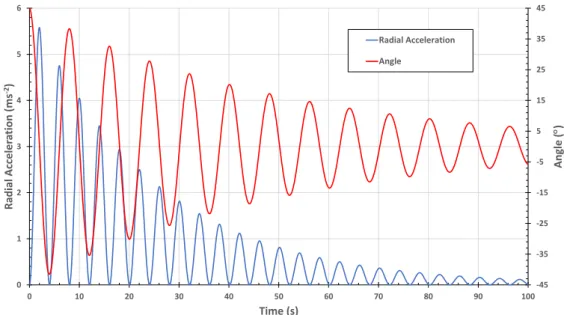
cen-tripetal acceleration. . . 11 3.3 Comparison of theoretical radial acceleration and angle of oscillation. Angle
calculated with equation 3.8. Acceleration calculated with equation 3.9. With these conditions:r= 16m,ω= 0.7826rad·s−1,θ0= 45◦ andτ= 45s. . . 13
3.4 The projected pendulum system. Thought out to be a build-it-yourself system using offthe shelf materials, while maintaining stability for a good oscillation. 1oscillating mass;2BITalino attached to the mass;3strings;4supports for the rods;5pivot rod;6metal rods for support. . . 14 3.5 Real pendulum experiment setup. BITalino attached to the oscillating mass. 15 3.6 Diagram of measuring radial acceleration on BITalino’s z axis. BITalino’s three
axis are drawn in white.. . . 15 3.7 The radial acceleration of an oscillating 0.600kg mass with a length of
oscil-lationr of 0.3m. . . 16 3.8 Detail of calculated minima and maxima. . . 17 3.9 The pendulum experiment GUI. For a complete rundown of all the buttons
and functionalities see Annex .. . . 18 3.10 The radial acceleration of an oscillating 0.600kg mass with a length of
oscil-lationrof 0.3m. The starting angle wasθ0= 65◦. In red, the local maxima of acceleration and in yellow the local minima. . . 19 3.11 MEMS accelerometer diagram. . . 19 3.12 z axis accelerometer behavior when the BITalino is stationary in three different
positions: a) BITalino is perpendicular to the resting position, in our pendulum system this is equivalent to a 90◦
angle; b) upside down BITalino; c) the resting position used for our measurements . . . 20 3.13 This is the type that is expected of the students to find. Two lines with acquired
L i s t o f F i g u r e s
3.14 Variation of the damping time versus the mass of the pendulum. Note that the proportionalityτ∝mexpected for viscous damping is not verified. . . 21
3.15 Angle of oscillation of a pendulum withr= 0.32m,m= 0.600kg. In blues the angle calculated using the minima of acceleration. In red the angles calculated using the maxima of acceleration. In black the theoretical curve. . . 22 3.16 Evolution of the period of one oscillation throughout the pendulum motion.
In blue dots the period of every oscillation, in red the average for 5 consecutive periods. The period of one oscillation is decreases with amplitude oscillation. 23 3.17 Period in seconds versus angle of oscillation in degrees. In blue, the raw data
and, in red, the averaged over 5 consecutive points data. Note the non-linear increase of the period for greater angles. . . 23 3.18 εin function of the squared angle. Plot made with the average of 5 consecutive
angles and time periods. . . 24 3.19 εin function of the squared angle. Plot made with the average of 5 consecutive
angles and time periods. In bluem= 0.600kg; in yellowm= 0.400kg; in red
m= 0.200kg. . . 25
4.1 Conductive ring in a static magnetic field . . . 28 4.2 Diagram of the experimental system. (1)is the induction system. (2)is an
electric rotor.(3)is a voltmeter. . . 29 4.3 Faraday induction experimental setup. . . 29 4.4 A two stage amplifier, for a total of 5151 gain, with a low-pass 1 Hz filter to
reduce noise. . . 30 4.5 The pre-amplifier assembled on a box. Banana connectors to connect to the
wire loops and a USB connector to connect the amplifier to BITalino. . . 31 4.6 Cutoff frequency response to different load resistances. Higher resistance
means the filter takes longer to act. . . 32 4.7 Typical plot of inducted tension in function of time. . . 33 4.8 The Faraday induction experiment GUI. . . 33 4.9 Voltage inducted, at constant speed and constant magnetic field intensity, on
a loop of varying widths: in red, a width of 0.040m; in blue width of 0.028m; and in yellow width of 0.02.0m. As predicted the voltage at width 0.040mis double the voltage inducted on a loop of 0.02.0mwidth.. . . 34 4.10 Voltage inducted on a loop of constant width, moving through a static
mag-netic field at different velocities: in red,v= 0.020m/s−2
; in bluev= 0.040m/s−2
; and in yellowv= 0.080m/s−2
. . . 35
5.1 Wheatstone bridge. Rx is where the Pt100 is connected. R3is the reference resistance. . . 40 5.2 Circuit schematic for temperature measurement with a Pt100 and a BITalino. 41 5.3 The effect of saturation of the LM 358 in red, as measured with a reference
resistanceR2= 93.2Ωand a gain of 10. In blue the output of an ideal opera-tional amplifier, for a circuit with the same reference resistance and gain. . . 42 5.4 The thermometer GUI. . . 43 5.5 Measured and theoretical temperatures in function of test resistances. . . 44 5.6 In blue the difference between measured and expected temperature, ∆T =
Tm−Te, in function of the Temperature. In black the gain of the circuit. . . . 45
5.7 Measured and theoretical temperatures in function of test resistances. . . 46 5.8 In blue the difference between measured and expected temperature, ∆T =
Tm−Te, in function of the Temperature. In black the gain of the circuit. . . . 46
L i s t o f Ta b l e s
2.1 BITalino plugged specifications, with an accelerometer installed. . . 5
2.2 Sensors used in Mechanics experiments. . . 7
2.3 Measurement equipment for Electromagnetism labs. . . 8
3.1 τfound for pendulum lengthr= 0.32m. . . 21
3.2 Linear fit equations for masses with pendulum lengthr= 0.32m.. . . 24
4.1 Cutofffrequency for different resistances. . . . . 31
4.2 Results obtained forv= 0.067m/sand 8 pairs of magnets, with varying loop width. . . 34
4.3 Results obtained for 8 pairs of magnets andb= 0.04m, with varying velocity. 34 4.4 Results obtained forv= 0.086m/sandb= 0.04m, with varying magnetic field intensity. . . 35
5.1 Theoretical bridge voltage for the two reference resistances used in section 5.2. 41 5.2 Measurement ranges and respective resolutions. . . 41
C
h
a
p
t
e
1
I n t r o d u c t i o n
1.1 Motivation
There have been great developments in both miniaturization of signal acquisition equip-ment and wireless data transmission. As these technologies become more accessible and
affordable, they open new possibilities in many areas. One such area is the development
of didactic material for physics labs.
Generally, the material required for experiments in introductory physics (Mechanics, Thermodynamics, and Electromagnetism) is sold by a handful of companies, such as LeyBold, Pasco, and Phywe. But this material has become costly. There is also a glaring compatibility problem, as components from one provider are usually not compatible with materials from another provider.
In this context, the goal of this thesis is to utilize new advancements in technology to develop new experiments and adapt old ones, while providing a lower cost and open source alternative to the commercially available didactic equipment. For this purpose, a partnership with PLUX, a Portuguese company that specializes in biomedical equipment for education and research applications, has been established. In the context of this thesis, PLUX provides access to equipment and technical support. The equipment provided is BITalino, a low-cost toolkit that has the required signal acquisition and wireless data transmission capabilities that is relatively inexpensive.
C H A P T E R 1 . I N T R O D U C T I O N
to measure temperature with a Pt100 resistance temperature detector.
1.2 Goals
The first goal of this project was to create a simple Graphical User Interface (GUI), in which a user can visualize the acquired data in real-time during the experiment. Another key aspect of using automatic data recording to enable the student to use a standard Excel worksheet for data analysis. Secondly it was determined which experiments, of those currently performed in labs of introductory physics courses, could best serve to exemplify BITalino’s didactic capabilities. Given that a great number of experiments can be done, it was decided to focus on two experiments. One can fully utilize the new acquisition board, the other takes advantage of the computerized acquisition system to further enhance the students’ access to information. The chosen experiments were: the study of the pendulum motion, and a Faraday induction study. A case study for making temperature measurements using a Pt100 resistance temperature detector and a BITalino, was performed.
1.3 Outline
In the present chapter the problem, motivation and overall goals of the work are intro-duced.
Chapter2explains why the pendulum and the Faraday induction experiments were
chosen, as well as a review of the most relevant commercially available solutions for these experiments. Also in this chapter, the BITalino board is introduced, with an overview of its technical properties.
Chapter3first introduces how an acceleration measurement system with wireless
capabilities brings forth new possibilities for the study of pendulum motion. It then proceeds to detail the experimental setup developed. To conclude it shows the acquired data, and how they compare with the elementary theory.
Chapter4introduces relevant concepts regarding how the Faraday induction
exper-iment is performed, and how using the BITalino makes it more visually appealing, and
lowers the cost. The chapter then proceeds to show how off-the-shelve components can
be used to build a ’homemade’ microvoltimeter. To conclude, experimental results show the feasibility of our solution using the BITalino and our ’homemade’ microvoltimeter.
Chapter5is a case study of how a simple circuit with a Pt100 and a BITalino could
be used as temperature measurement equipment.
Finally, Chapter6outlines the main conclusions of this work, and provides insights
C
h
a
p
t
e
2
C o n t e x t ua l i z a t i o n
This chapter presents an overview of the state-of-the-art on existing tools for physics didactic experiments. Secondly, the choice of the BITalino acquisition board is justified, presenting relevant technical characteristics. Finally, an overview of the experiments done on introductory physics labs at FCT/UNL.
2.1 Didactic Physics Labs
Lab experiments are a key part of learning physics. Some studies suggest that they help with retention ability [1], foster critical-thinking abilities [2], and teach students to test
and evaluate models [3]. The use of hands-on lab experiments for increasing student
performance is still up for debate, however [4] suggests it does not systematically increase
students performances on final exams.
As an alternative to hands-on labs, there are simulation based labs. Recent studies
suggest that students learn equally well from either type of experience [5]. In the same
study it was found that the biggest difference between hands-on and simulation labs is in
the perception of the students. While the conclusions cannot be generalized, students in this study felt they learn better from hands-on experiences.
However, lab experiments, either hands-on or simulation, are still widely used. Al-most every undergraduate, as well as high school, level physics class features lab assign-ments in which the students are expected to apply knowledge, acquired in theoretical classes, to a practical example. A market exists to facilitate access to equipment for these labs, and, as technology evolves, so must the experiences.
C H A P T E R 2 . C O N T E X T UA L I Z AT I O N
of the acquisition boards mentioned before, there is a corresponding program to control the board, and visualize data. Each interface only works with sensors of their respective brand.
Developments in both miniaturization of signal acquisition equipment and wireless data transmission open new possibilities in many areas. PLUX has developed BITalino,
which is a low-cost toolkit to learn and prototype applications using body signals [6].
This new facet of acquisition boards comes about from a global revolution in the way the physical and the digital world interact, which, itself, is closely related to the
’do-it-yourself’ movement. The popularity of Arduino and Raspberry Pi are proof of this [7].
An example of the do-it-yourself mentality is the Creator Kit from Fritzing company [8],
which provides an introduction to do-it-yourself electronics. Another similar kit is the
Sparkfun Inventor’s Kit - V3.3 which provides basic electronic components for $100 [9].
2.2 BITalino
(a)
I1
PWM O2/I2
O1
A4
A3
A2
A1
A5
A6
ACC
(b)
Figure 2.1: The BITalino plugged hardware configuration2.1a, adapted from [10]. The
board mounted on a 3D printed case2.1b.
PLUX has commercialized its low-cost (starting at 149€+ shipping) acquisition board
BITalino since August 2013. BITalino’s low-cost was thought out as a community
mo-tivator, it was not designed to be a money-maker [11]. The hardware consists of a low
cost, modular wireless biosignal acquisition system with a credit card-sized form factor. The motivation behind using BITalino comes from these three conditions. The wireless acquisition system is an interesting concept that might prove to be useful in developing new experiments, namely in Mechanics experiments. The small dimensions of the system and the wireless acquisition system allow for implementation in a greater number of experiments. Additionally, BITalino has a whole set of available software tools that lets a greater number of people just pick it up and start developing new things. All this for an
BITalino has three different configurations available for purchase,Board, Plugged, and Freestyle[6,12]. Figure2.1bdisplays the plugged configuration used on our work. In this
configuration plugs are added to BITalino’s ports. Table2.1presents the specifications of
the individual blocks, provided by default on the analog front-end. BITalino was designed to have a set of generic analogue ports, in this way it is possible to connect sensors with analog outputs. Moreover, it is possible to develop specific sensors for many applications, and connect them to BITalino.
Table 2.1: BITalino plugged specifications, with an accelerometer installed.
Specifications
Sampling Rate Configurable to 1, 10, 100, 1000 Hz
Analog Ports 4 input (10 bit) + 2 input(6 bit)
Digital Ports 1 input (1 bit) + 4 output(1 bit)
Data link Class II Bluetooth v2.0 ( 10 m range)
Actuators LED
Sensors Tri-axial accelerometer
Weight 30 g
Size 100 x 60 mm
Battery 3.7 V LiPo
Consumption 65 mAh (with all peripherals active)
The ports enumerated in table2.1are identified on the board as per figure2.1b. Ports
I1, O2,andI2/O2are digital input and output ports. PWMis a pulse width modulator,
usually used to control a digital-analog converter. PortsA1-A6are the analog ports, of
whichA5andA6are 6 bit input ports and the others are 10 bit input ports. On the board
used in this work, we connected a tri-axial accelerometer (ACCto portsA1, A2,andA3
(one port for each axis of measurement) as can be seen in figure2.1b. We used the 10 bit
analog portA4to connect different sensors.
BITalino has several application programming interfaces (API) that allow to easily incorporate BITalino in custom made software applications. In the context of this work we used the Python API.
2.3 Physics Labs at FCT/UNL
Whether developing new or adapting old experiences, we are looking to make better
and/or more affordable experiments. In this context, why is the pendulum the model
C H A P T E R 2 . C O N T E X T UA L I Z AT I O N
2.3.1 Mechanics
The FCT/UNL Mechanics laboratory class of the Physics Department is equipped to perform a total of 13 experiments:
1. Average velocity;
2. Newton’s 2nd law;
3. Projectile motion;
4. Angular momentum;
5. One dimensional collisions;
6. Two dimensional elastic collisions;
7. Rotational collisions;
8. Centrifugal force;
9. Simple Pendulum;
10. Compound pendulum;
11. Ballistic pendulum;
12. Non isochronous pendulum;
13. Ideal spring.
In table2.2the necessary sensors for each of these experiments are enumerated. In
the far right column it is also indicated if the acquired data are immediately sent to a computer.
All these experiments use PASCO Scientific equipment and software (DataStudio). This equipment was bought a few years ago, since then PASCO has updated its catalog, introducing new equipment and discontinuing some of its old equipment. PASCO also developed a new interface software, PASCO Capstone , and stopped updating their
previ-ous DataStudio software [13]. This means new hardware does not work with old software.
For instance, the PASPORT Motion Sensor PS-2103A requires the PASCO 850
Univer-sal Interface in order to visualize the data [14]. The 850 Universal Interface, however,
does not work with the old DataStudio software and requires PASCO Capstone software
[15]. This reveals another advantage of using open source equipment. Anyone with the
necessary expertise can adapt what has been done before to their own needs.
Table 2.2: Sensors used in Mechanics experiments.
Motion Sensor Timer Photogates Sonar Computer
Average velocity - 1 - 2
-Newton’s 2nd law - - - 1 X
Projectile Motion - - - -
-Angular momentum - 1 1 -
-One dimensional collision - 2 2 2 X
Two dimensional collision - - - -
-Rotational collision 1 - - - X
Centrifugal force - 1 - -
-Simple Pendulum - 1 - 1
-Compound pendulum - - 1 1
-Ballistic pendulum - 1 2 -
-Non isochronous pendulum 1 - - - X
Ideal Spring - - - 1 X
Total 3 5 5 9
collision for instance, through a measurement in acceleration. It might then be possible to adapt this experiment to work with acceleration measurements.
In Mechanics experiments, one advantage of the BITalino with an accelerometer equipped is in fact the wireless data transmission capability, which makes it possible to attach the board to a moving object and record data with no topological drawbacks from attached wires. This is the case for pendulum based experiments, this being the main reason why the real pendulum experiment is the model experiment in this work.
The simple and compound pendulum experiments performed are not quite up to par with the richness of this system. They consist of using a timer and a photogate to measure the period of one pendulum oscillation. The period is then used to determine free fall
acceleration on the surface of the Earth,g. However, a pendulum experiment can be used
for more. For instance, to study harmonic oscillation, and to study the effect of damping.
By attaching the BITalino to the oscillating mass and measuring the acceleration, we propose that a new pendulum experiment that can be designed to more extensively study its motion. At the same time, this makes the experimental setup much simpler, as will be
described in chapter3.
2.3.2 Electromagnetism
The FCT/UNL Electromagnetism lab is equipped to perform a total of 6 experiments:
1. The oscilloscope;
2. Tracing electric field equipotential lines;
C H A P T E R 2 . C O N T E X T UA L I Z AT I O N
4. Charge and discharge of capacitors;
5. Electron trajectories in a magnetic field;
6. Faraday induction 1, conductive ring moving through a magnetic field;
7. Faraday induction 2, magnetic flux variations by means of a coil;
In table2.3the necessary measurement equipment is enumerated.
Table 2.3: Measurement equipment for Electromagnetism labs.
Voltmeter Ammeter Oscilloscope Timer Computer
Oscilloscope - - 1 -
-Equipotential lines 1 - - -
-DC circuits 1 1 - -
-Capacitor - - 1 -
-Electron trajectories - - - -
-Faraday induction 1 1 - - 1
-Faraday induction 2 1 1 - -
-Total 4 2 2 1
Some of these experiments are inherently made to be used with certain equipment. The oscilloscope experiment’s goal is to familiarize the student with the oscilloscope func-tionalities. It is therefore absolutely necessary to use the oscilloscope. The equipotential lines are supposed to be drawn on paper by the student. The electron trajectories ex-periment is the exex-periment that requires the most material, but the students are only requested to measure diameters of circular trajectories versus magnetic fiend and acceler-ation potential.
The remaining experiments could have their measurement tools replaced by a BITal-ino. However, BITalino has a few limitations that, at this time, make some of these
experiments difficult to adapt. These experiments are the capacitors experiment and the
Faraday induction 2. They concern phenomena that happen in a frequency range higher
than BITalino’s highest sampling rate (1000Hz). The charge frequency on the RC circuits
tested is on the order ofkHz, and the frequency of the Faraday induction experiment is
in the 100−2000Hzrange.
Thus, we chose the Faraday induction 1 experiment because this experiment needs to measure microvolts and it does not have the limitations mentioned above. The BITalino does not have the necessary resolution to measure voltage in the order of microvolts, for this reason a pre-amplifier must be built, giving the chance to embrace the do-it-yourself mentality. Applying the BITalino to this experiment also makes a few other improvements
C
h
a
p
t
e
3
P e n d u l u m
In this chapter the pendulum experiment will be described. Firstly, a theoretical
contex-tualization is made in section3.1. This experiment has two objectives. The first objective
is to experimentally determine the damping time constant,τ, of a real pendulum. The
sec-ond objective is to demonstrate that for a real pendulum the oscillation period depends on the angle.
Secondly, the experimental setup is presented in section3.2. What is new about our
experiment design is that the BITalino with an equipped accelerometer is part of the oscillating body. The board itself can oscillate because there are no wires to connect the accelerometer to the acquisition board. With this setup the measured quantity is acceleration. However, thinking in terms of acceleration is not intuitive: our mind is more trained to analyze position or velocity variations than acceleration variations.
In section3.3results and discussion are presented. The acquired acceleration data are
plotted and compared to theoretical data. It is shown how, utilizing, the acquired data it is possible to achieve the proposed goals of the experiment.
3.1 Theoretical Formulations
3.1.1 Acceleration of an Ideal Pendulum
The pendulum is an example of a non-uniform circular motion. It consists of an object
of mass m attached to the end of a string of length r. The other end of the string is
attached to stationary point. θis the angular position of the object, with respect to the
downward vertical, see figure3.1. If damping forces are neglected, it can be deduced that
the differential equation3.1describes the motion of a simple pendulum.
d2θ
dt2 +
g
C H A P T E R 3 . P E N D U LU M
r
mg
mgsin mgcos
mg
Figure 3.1: A pendulum representation.
in whichgis the gravitational acceleration. Making use of the small angle approximation,
sinθ≈θ, expression3.1 becomes the expression for the angular movement of an ideal
pendulum:
d2θ
dt2 +
g
rθ= 0 (3.2)
equation3.2is the differential equation for a simple oscillatory movement with angular
frequencyω=
q g
r. A possible solution for this equation is:
θ(t) =θ0cos(ωt+φ) (3.3)
φ is the initial phase of the movement,θ0is the amplitude of the movement. φandθ0
are initial conditions of the movement. For simplicity’s sake, we will considerφ= 0: this
condition implies that the pendulum is dropped from its maximum amplitude att= 0.
Thus,θ(t) =θ0cos(ωt) is the equation that describes the angular motion for a small
angle ideal pendulum. It follows that the pendulum has radial, vr, and tangential,vθ,
velocities given by:
vr= ˙r (3.4)
vθ=rθ˙ (3.5)
becauser is constant,vr = 0. The radial (or centripetal) and tangential acceleration are,
respectively, given by:
ar= vθ 2
r (3.6)
3.1.2 Acceleration of a Real Pendulum
The first objective of this experiment is to determine the damping time constant of a real
pendulum. Introducing viscous damping to equation3.2 makes it so the amplitude of
movement decreases exponentially. A solution to this equation can be:
θ(t) =θ0cos(ωt) exp(−t/τ) (3.8)
replacing3.8in eq.3.6, we get the radial acceleration given by3.9:
ar=rθ02exp −2t/τ
"
ωsin(ωt) +cos(ωt)
τ
#2
(3.9)
thinking in terms of acceleration is not common and usually not very intuitive. At the position where the tangential velocity is zero, the centripetal acceleration of the
pen-dulum given by vθ2
r is also zero, as seen in figure3.2 Therefore, at this point the force
along the radial axis should be less than when the pendulum passes through its resting position, where the centripetal acceleration is at its maximum. Thus, there is a radial
acceleration maximum whenever the pendulum passes the position whereθ= 0. Because,
during a full oscillation, the pendulum crosses this point twice, there are two maxima of acceleration for each pendulum oscillation. The same happens for minima of acceleration. This reasoning implies that the frequency of the radial acceleration is twice that of the angle. Mathematically, this frequency doubling comes from the fact that this acceleration
is calculated as the square of an harmonic oscillation, as shown in equation3.9.
To the acceleration caused by the gravitational force we must add the centripetal
acceleration of a circular motion. In figure 3.2we see that the centripetal acceleration
is null when the pendulum reaches its maximum angle. The centripetal acceleration
is always zero when the object is stationary. When the pendulum crosses θ = 0 the
centripetal acceleration is maxed.
max
𝒈 cos 𝜃𝑚𝑎𝑥 𝒗
𝟐
𝒓 > 𝟎 𝒗𝟐
𝒓 = 𝟎
𝒈
C H A P T E R 3 . P E N D U LU M
In the case of low damping, the radial acceleration can be calculated for the two
extreme cases whereωt=nπandωt=nπ+pi/2.
Forωt=nπ:
sin(nπ) = 0 cos(nπ) =±1 (3.10)
ar=rθ0 2
τ2 exp(−2t/τ) (3.11)
forωt=nπ+π/2 :
sin(nπ+π/2) =±1 cos(nπ+π/2) = 0 (3.12)
ar=rθ02ω2exp(−2t/τ) (3.13)
at the same time, replacingωt=nπ∨ωt=nπ+π/2 on equation3.8it results in:
θ(nπ) =θ0cos(nπ) exp −t/τ
=±θmax (3.14)
θ(nπ+π/2) =θ0cos(nπ+π/2) exp −t/τ
= 0 (3.15)
the radial component of the gravitation force is maximized when the pendulum is atθ= 0,
thus the radial acceleration is maxed at this angle. Figure 3.3 shows the relationship
between angle and radial acceleration.
We can now say that to findτ we only need to knowr,ω,θ0and the maxima of radial
acceleration. We expect these maxima to vary withexp(−2t/τ). Therefore, if a plot is made
of the experimental and theoretical maxima it is possible to adjust τ on the theoretical
data so that it matches the experimental results.
3.1.3 Period of a Real Pendulum
The second objective of this experiment is to verify that the period of oscillation of a real
pendulum depends on the angle of oscillation if the conditionθ≪1 is not verified. In
this case, the period of a pendulum can be approximated by:
T = 2π
r
r g
1 + 1
16θ0
2+ 1
3072θ0
4+· · · (3.16)
in this expression it is also possible to see the small angle approximation, ifθ ≪1 the
latter contributions of the series are negligible. These latter contributions can be
con-sidered corrections to the small angle approximation. So,T0= 2π
qr
g is the small angle
approximation, addingT1=T0·161θ02would be a first correction to the approximation,
and so on with the following terms of the series.
-45 -35 -25 -15 -5 5 15 25 35 45 0 1 2 3 4 5 6
0 10 20 30 40 50 60 70 80 90 100
Angle ( ) Ra dial Acceler a tion (ms -2) Time (s) Radial Acceleration Angle
Figure 3.3: Comparison of theoretical radial acceleration and angle of oscillation. Angle
calculated with equation 3.8. Acceleration calculated with equation 3.9. With these
conditions: r= 16m,ω= 0.7826rad·s−1,θ0= 45◦andτ= 45s.
• The period is not constant but decreases with time. Or rather, the period decreases as the amplitude decreases;
• And then show how this dependency follows equation3.16.
3.2 Experimental Setup
3.2.1 The Pendulum System
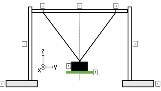
The planned pendulum system is shown in figure3.4. The idea here is to have an
oscillat-ing mass (1) with an attached BITalino (2). Mass (1) is attached to one end of two stroscillat-ings (3) suspended from a pivot rod (5). Rod (5) is secured in place by two clamps, one for each rod (6). Finally, supports (4) give stability to the entire system.
The system uses two strings to force oscillation to occur on the (x, z) plane. Ideally,
with one string the oscillation starts with the mass at a 90◦
angle between axis x and y.
As a matter of fact, with a pendulum using only one string, it would be very difficult to
avoid oscillations in the y direction: the analysis of the motion becomes more complicated without adding any didactic information. Therefore, the mass is suspended from two strings to limit oscillations on the (z, y) plane.
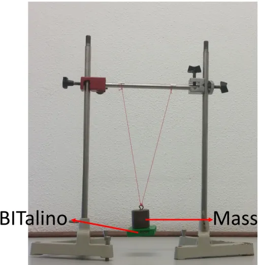
Figure3.5 shows a photograph of the built system. All the materials were re-used
C H A P T E R 3 . P E N D U LU M
2 1
3 3
4 4
5
6 6
y
x
z
Figure 3.4: The projected pendulum system. Thought out to be a build-it-yourself system
using offthe shelf materials, while maintaining stability for a good oscillation.1
oscillat-ing mass;2BITalino attached to the mass;3strings;4supports for the rods;5pivot rod;
6metal rods for support.
in the motion. Possible solutions would be to either use heavier supports or to fix the supports to the working station.
The strings should have the same length but because of the knots’ quality it might happen that, during the oscillation of the pendulum, one of the knots gets loose and stretches. This causes the pendulum to skew to one side causing the oscillation to occur in more than two directions. Because the strings are tied to the horizontal bar, we need to make sure they do not slide across the bar during oscillation. We decided to fix them by putting tape on top of the knot and over the bar. An improvement to this issue would be to drill two holes on the horizontal bar and to pass the strings through the bar. This
would also make it easier to adjust string length for different experiments.
In regards to the BITalino attachment, because it has a tri-axial accelerometer there is some flexibility as to where it can be attached. In this build, it was found best to attach the BITalino to the bottom of the mass, and so the accelerometer will measure the radial acceleration on its z-axis, see figure3.6.
3.2.2 Python Program: Pendulum Data
The function that transforms digital value sampled, ADC, to acceleration in g, ACC,
called a transfer function, is given in the accelerometer datasheet (AnnexII):
ACC(g) =ADC−Cmin
Cmax−Cmin
·2−1 (3.17)
where ADC is the digital value sampled, in bit.Cmin andCmaxare the values, in bit,
BITalino
Mass
Figure 3.5: Real pendulum experiment setup. BITalino attached to the oscillating mass.
x
z
𝑔 cos 𝜃
𝑔
C H A P T E R 3 . P E N D U LU M
before the experiment is made. In Annex III we describe how to calibrate BITalino’s
accelerometer.
The resulting data from a pendulum motion are plotted using Excel to obtain figure
3.7. This data will be further discussed in section3.3.
0 2,5 5 7,5 10 12,5 15 17,5 20 22,5 25
0 20 40 60 80 100 120 140 160 180 200 220 240 260 280 300
Acceler
a
tion (ms
-2)
Time (s)
Figure 3.7: The radial acceleration of an oscillating 0.600kg mass with a length of
oscil-lationrof 0.3m.
As previously discussed, there is interest in finding the local maxima and minima
of the acquired data. As this would be a relatively difficult task to give to a student in
Introductory Physics, the program finds and registers these points when the data are saved.
A Python script smooths the data to facilitate peak finding. A different script then
finds the points in time at which peaks occur. The time at which the smoothed maxima
and minima occur is the same as in the original data. Figure3.8shows how the maxima
and minima calculated by the script are in good agreement with the acquired data.
We have already mentioned how a period of oscillation has two maxima and two
minima of acceleration. This is why, in Figure3.8, we only mark every other maximum
and minimum. This allows for the student to obtain directly in a file the value of the oscillation motion versus time without any complicated treatment. As we have seen
a single acceleration period comprises two minima, corresponding to ±θmax, and two
maxima, because the oscillation crosses θ = 0 twice. This makes it easier to treat the
0 2,5 5 7,5 10 12,5 15 17,5 20 22,5 25
0 0,5 1 1,5 2 2,5 3 3,5 4 4,5 5 5,5 6 6,5 7 7,5
Acceler a tion (ms -2) Time (s) Acceleration Data maxima minima
Figure 3.8: Detail of calculated minima and maxima.
3.2.3 Python Program: Graphical Interface
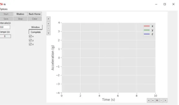
Figure 3.9shows the graphical user interface (GUI) for the pendulum experiment. Its
primary function is to show acquired data in real-time. There is also an option for calibrating the accelerometer. For the first stage of this work, the GUI was made with no concern for looks. The priority was to build a robust program that would allow for data visualization in real time.
The program has asavebutton which creates an Excel file with two sheets, as well as a
text file. The first sheet has all points of acceleration acquired. The calibration values can be used, in conjunction with the raw data, to retrace the steps in finding the maxima and minima. The other has the maxima and minima, as well as corresponding time stamps. The text file has the raw data acquired by the BITalino and a header with information
like: sampling rate, total acquisition time,Cmin andCmax.
There are two possible ways to visualize data being acquired:
• Window mode. In this mode the plot will always show the data recorded during
the lastXseconds. The amount ofXtime shown is set in theInterval (s)entry field.
There is, at this time, no possibility to see data that has already passed.
• Complete mode. In this mode data are acquired during a set amount of time. The
amount of time is controlled by the entry fieldInterval (s).
3.2.4 Laboratory Guide
An experiment guide was written (AnnexIV), in it there is a step by step guide on how
to setup the experiment and how to setup the visualization program.
The guide starts off stating the objectives for the experiment. Next it makes a
C H A P T E R 3 . P E N D U LU M
Figure 3.9: The pendulum experiment GUI. For a complete rundown of all the buttons and functionalities see Annex .
is also a section explaining how to use the program, including how to calibrate the ac-celerometer.
3.3 Results and Discussion
3.3.1 Results
The results presented here will follow the necessary steps to complete the experiment
and complete the objectives. The resulting acceleration data of a 300spendulum motion
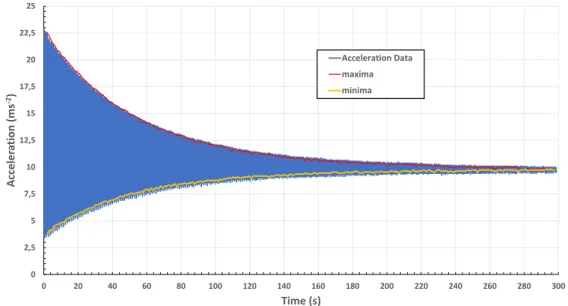
with our system are plotted in figure3.10. It is also shown the maxima and minima found
by our program. All figures in this section are from the same motion of a 0.600kg mass
suspended on a 0.3mlength string.
The radial acceleration was expected to be 0 at its minima. And in figure3.10 it is
observed this is not the case. Why? Because of the type of accelerometer installed on the BITalino. This accelerometer is a micro electro-mechanical system (MEMS) consisting of
a cantilever and a strain sensitive resistor (Fig.3.11). This type of accelerometer relies on
0 2,5 5 7,5 10 12,5 15 17,5 20 22,5 25
0 20 40 60 80 100 120 140 160 180 200 220 240 260 280 300
Acceler a tion (ms -2) Time (s) Acceleration Data maxima minima
Figure 3.10: The radial acceleration of an oscillating 0.600 kg mass with a length of
oscillation r of 0.3 m. The starting angle was θ0 = 65
◦
. In red, the local maxima of acceleration and in yellow the local minima.
Mass Fixed frame Cantilever Strain sensitive resistor
y
x
z
F=maFigure 3.11: MEMS accelerometer diagram.
Our pendulum setup has the BITalino attached to the oscillating mass so that the
z axis accelerometer measures radial acceleration (Fig.3.6). From the point of view of
the acceleration due to motion, we could expected the acceleration measured when the pendulum is at rest to be 0. But this is not the case because the cantilever is actually measuring a force. At rest, the z axis accelerometer measures the gravitational force, as
can be seen in figure3.12.
Still, even with this consideration we expected that the minima should beg. And,
once again, this is not the case. While the tendency of the acceleration is to reachg, at
the beginning of the motion the minima are lower than g. This too is a consequence
of the cantilever accelerometer. When the pendulum hits its maximum amplitude the
BITalino itself is inclined, exactly as shown in figure3.6. Because of this inclination, the
gravitational force acting upon the z axis cantilever is no longer given byFg =mg, but
rather by Fg =mgcosθ. Therefore, even if the radial acceleration of the pendulum is
C H A P T E R 3 . P E N D U LU M
y
x
z
a)
b)
c)
BITalino BITal ino BI Tal ino BI Tal inomg
mg
mg
Figure 3.12: z axis accelerometer behavior when the BITalino is stationary in three dif-ferent positions: a) BITalino is perpendicular to the resting position, in our pendulum
system this is equivalent to a 90◦
angle; b) upside down BITalino; c) the resting position used for our measurements
a=gcosθ. This peculiarity turns out be quite useful as it allows a different measurement
of the angleθmaxgiven by:
a=gcosθmax (3.18)
θmax= arccos a
g ! (3.19) 0 2,5 5 7,5 10 12,5 15 17,5 20 22,5 25
0 25 50 75 100 125 150 175 200 225 250 275 300
Acceler a tion (ms -2) Time (s) Experimental Maxima Experimental Minima Theoretical Minima Theoretial Maxima
Figure 3.13: This is the type that is expected of the students to find. Two lines with
acquired maxima and minima. And two lines where the student must find the τ that
3.3.2 Findingτ
The first objective of the pendulum experiment is to find the damping time constant,τ, for
different masses and different lengths of oscillation. We need to obtain theoretical curves
that closely match the experimental maxima and minima. There are two ways to achieve
this: a) use equation3.13, adding the offsetg= 9.8m/s2, to find theoretical maxima in
function ofτ; b) or by using equation3.18. The latter requires an extra step of finding
theoretical values for the angle at each minimum time, using expression 3.9. In figure
3.13it is seen a plot, forτ= 115s, with both the experimental and theoretical curves. The
optimalτ is found by trying differentτ values until the theoretical curves closely match
the experimental . In figure3.13 we show an example of this, these theoretical curves
haveτ = 115 s. Table 3.1shows typical values ofτ for different masses and lengths of
oscillation.
Table 3.1:τfound for pendulum lengthr= 0.32m.
Mass (kg) τ(s)
0.600 115
0.400 130
0.200 140
If the damping factor is originated from viscous damping, the time constantτshould
be proportional to the mass of the pendulum. In figure3.14it is shownτin function of
the oscillating mass. There is no agreement with τ being proportional to the mass. So
we conclude that viscous damping is not the main damping source for attenuation of the pendulum motion.
y = -62,5x + 153,33
0 10 20 30 40 50 60 70 80 90 100 110 120 130 140 150 160 170
0 0,05 0,1 0,15 0,2 0,25 0,3 0,35 0,4 0,45 0,5 0,55 0,6 0,65
τ
Mass (Kg)
r = 0.32 m
Figure 3.14: Variation of the damping time versus the mass of the pendulum. Note that
C H A P T E R 3 . P E N D U LU M
3.3.3 Period of a Real Pendulum
During the entire motion of the pendulum there will be several single oscillations. This can be taken advantage to reach our second objective, which is to verify that the period of
one oscillation depends on the angle of oscillation, according to equation3.16. Because
we are interested in the period of only one oscillation, we can assume that there is no damping for the duration of a single oscillation. With this and the acceleration maximum
amax calculated by our program, we can calculate the angle amplitudeθ0for each single
oscillation with expression3.20. This expression is derived from equations3.3and3.6:
θ02=amax
rω2 (3.20)
As mentioned in the previous section, there is a different way to findθ0. Which uses
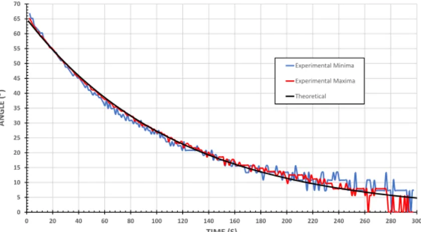
BITalino’s inclination when the mass reaches its maximum amplitude. Figure3.15shows
a comparison between the angle calculated in both ways, using both maxima and minima
of acceleration. In this figure is also plotted the theoretical curve, withτ= 115s.
0 5 10 15 20 25 30 35 40 45 50 55 60 65 70
0 20 40 60 80 100 120 140 160 180 200 220 240 260 280 300
ANG LE ( ) TIME (S) Experimental Minima Experimental Maxima Theoretical
Figure 3.15: Angle of oscillation of a pendulum withr= 0.32m,m= 0.600kg. In blues
the angle calculated using the minima of acceleration. In red the angles calculated using the maxima of acceleration. In black the theoretical curve.
Results show strong agreement between angle calculated using experimental data, and the expected theoretical results. There is even good agreement between results using the minima and the maxima of acceleration. At the end of the motion it can be seen some discrepancy. At this point of the motion, the oscillation is very subtle. Therefore the variation in acceleration is lower than BITalino’s resolution. This in turn makes it impossible for our program to properly detect either maxima or minima.
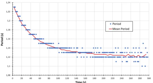
The period of each oscillation is calculated by our program. Since we save the time at which each maximum occurs the period is just the time between two consecutive
maxima. Figure 3.16 shows the calculated period as function of time and the mean
period calculated for 5 consecutive oscillations. As predicted by expression 3.16, for
exhibits a tendency towards a constant. This constant value corresponds to the time period for a small angle oscillation.
1,08 1,1 1,12 1,14 1,16 1,18 1,2 1,22 1,24
0 20 40 60 80 100 120 140 160 180 200 220 240 260 280 300
P eriod (s) Time (s) Period Mean Period
Figure 3.16: Evolution of the period of one oscillation throughout the pendulum motion. In blue dots the period of every oscillation, in red the average for 5 consecutive periods. The period of one oscillation is decreases with amplitude oscillation.
Since variation of both the angle and period of a single oscillation behave as expected throughout the motion there should be a correlation between angle and period of
oscilla-tion. In figure3.17we plot period of oscillation versus angle amplitude using the data of
figures3.15and3.16, the dependence of the period versus the amplitude can be obtained.
To test the correlation, the termε= T−T0
T0 is introduced. Where T is the measured
period. This term can be related to equation3.16by consideringT0= 2π
qr
g, giving:
1,08 1,1 1,12 1,14 1,16 1,18 1,2 1,22 1,24 1,26
0 5 10 15 20 25 30 35 40 45 50 55 60 65 70
P
eriod
(s)
Angle ()
Raw Data Averaged Data
C H A P T E R 3 . P E N D U LU M
T =T0
1 + 1
16θ0
2+ 1
3072θ0
4+· · · (3.21)
From this expression we see thatT should be dependent of the squared angle, in radians.
If we consider only the first squared term, we get thatT should be linearly dependent of
the squared angle:
T =T0
1 + 1
16θ0
2 (3.22)
This expression can then related to the termεby:
T−T0
T0
= 1
16θ0
2 (3.23)
Figure3.18shows a linear fit ofεin function of the squared angle of oscillation. In
theory, the slope of this fit should be the coefficient of equation 3.23. The predicted
coefficient is 0.0625 and the fit gives 0.0785, which is in the same order of magnitude of
the expected value.
y = 0,0785x + 0,0003
0 0,01 0,02 0,03 0,04 0,05 0,06 0,07 0,08 0,09 0,1 0,11
0 0,1 0,2 0,3 0,4 0,5 0,6 0,7 0,8 0,9 1 1,1 1,2 1,3
ε
2(rad2)
Figure 3.18: εin function of the squared angle. Plot made with the average of 5
consecu-tive angles and time periods.
In figure3.19we plotεversus the squared angle of oscillation for the a pendulum with
three different masses. The linear fit for each of these masses gives equations shown in
table3.2. The coefficient found by the linear fit is very similar for each of these oscillation.
Table 3.2: Linear fit equations for masses with pendulum lengthr= 0.32m.
Mass (kg) Linear Fit
0.200 ε= 0.0787θ2+ 0.0002
0.400 ε= 0.0798θ2+ 0.0004
0 0,02 0,04 0,06 0,08 0,1 0,12
0 0,1 0,2 0,3 0,4 0,5 0,6 0,7 0,8 0,9 1 1,1 1,2 1,3
ε
2(rad2)
600g 400g 200g
Figure 3.19: εin function of the squared angle. Plot made with the average of 5
con-secutive angles and time periods. In bluem= 0.600kg; in yellowm= 0.400kg; in red
C
h
a
p
t
e
4
Fa r a d ay I n d u c t i o n : M e a s u r i n g M i c r o v o lt s
w i t h B I Ta l i n o
In this chapter we describe an experiment that verifies Faraday’s induction law. This is done by measuring the tension inducted on a coil moving through a stationary magnetic field. The tension is measured in function of magnetic field intensity, area, and velocity.
We aim to make improvements in measurement visualization and cost. Currently, at the FCT-UNL physics laboratory, this experiment uses a very flexible voltmeter, it has
many possible ranges of measurement, from [−100,100] µV to [−3,3] V. However, the
visual reading is made with a pointer, this may lead to inaccurate measurements. Our goal is to facilitate more precise measurements of tension, and, at the same time, to provide the data recorded in a file in order to have a more reliable treatment.
In section4.1a theoretical contextualization is presented. Section4.2shows the setup
for this experiment. And results of this experiment using the BITalino are presented in section4.3.
4.1 Theoretical Formulations
Faraday’s law of induction says that when the magnetic fluxΦthrough a surfaceA, whose
boundary is a wire loop, changes, the wire loop acquires an electromotive forceε, which
is given by the rate of change of the magnetic flux over time:
ε=−d
Φ
dt (4.1)
The change in flux can be cause either by changing the intensity of magnetic fieldB,
C H A P T E R 4 . FA R A DAY I N D U C T I O N : M E A S U R I N G M I C R OVO LT S W I T H
B I TA L I N O
b
ε
Figure 4.1: Conductive ring in a static magnetic field
Φ=
Z
~
B·d ~A (4.2)
In this experiment the wire loop is moved out of a uniform magnetic field at constant
velocityv. The surface area inside the field varies, therefore so does the magnetic flux.
An electromotive forceε, proportional to the flux variation is, in this way, created on the
wire loop. The loop used in this experiment has a rectangular form of widthb, see figure
4.1. Thus the flux variation with time is given by:
dΦ
dt =B dA
dt (4.3)
And so, combining expressions4.2and4.3we get:
ε=Bbv (4.4)
this expression indicates proportionality between the electromotive force created in the
loop, ε and three variables. To verify proportionality with magnetic field intensity B,
the intensity of the magnetic field can be changed by changing the number of magnets.
Proportionality betweenεand velocityv can be tested by moving the loop at different
speeds. Lastly, the relation between areaAandεcan be verified by changing the widthb
of the loop.
4.2 Experimental Setup
4.2.1 System Summary
Figure4.2shows a diagram of this experiment setup. Induction system(1)is the structure
in the wire loop moves through the magnetic field. The magnetic field is created by
magnets laid out in pairs. The wire loop is mounted on a cart pulled by rotor(2)at a
constant speed controlled by a power source. There are 3 different sized loops, which can
2
3
Figure 4.2: Diagram of the experimental system. (1)is the induction system. (2)is an
electric rotor.(3)is a voltmeter.
In this experiment the induced tension can vary from 20 µV to 300 µV. BITalino
has a resolution of 10 bit with an input range of up to 3.3V. This means that BITalino’s
smallest measurement is of around 3mV. Then, it is not possible to directly use BITalino
to measure the tension induced on the wire loop. For this reason, it is necessary to build an electronic circuit that amplifies the induced voltage.
In Figure4.3we see the assembled experimental setup for this experiment. There are
a few additions to what is shown in Figure4.2: a switch to turn the rotor on and off, and
the BITalino connected to the pre-amplifier which is connected to the wire loop. BITalino sends the voltage data to a computer connected via Bluetooth. In this setup, the desk microvoltmeter is still used to verify that the data measured with BITalino are identical to what is read by the microvoltmeter. In the final experimental setup for the lab the desk microvoltmeter will not be used.
Microvoltmeter
Pre-amplifier BITalino Switch
C H A P T E R 4 . FA R A DAY I N D U C T I O N : M E A S U R I N G M I C R OVO LT S W I T H
B I TA L I N O
4.2.2 Circuit Dimensioning
As was mentioned, it was necessary to build an electronic circuit. The final circuit is
shown in Figure4.4.
Figure 4.4: A two stage amplifier, for a total of 5151 gain, with a low-pass 1 Hz filter to reduce noise.
The circuit uses two INA 333 instrumentation amplifiers. These amplifiers are spe-cialized for low power functionality, featuring low power single-supply and rail-to-rail
output [16]. This means they are perfect to use with the BITalino.
The BITalino can supply either 3.3V or 1.65 V of output power. Having the
inter-mediate point 1.65V gives some flexibility in designing the circuit. Our goal with this
circuit is to measure a range of [−300; +300]µV with BITalino.
The circuit is a two stage pre-amplifier. On the first stage, the difference between the
two extremities of the loop is amplified by a gain of 101. Vee = 1.65V are supplied to
this amplifier’s reference pin, and to the loop. The latter is needed because the inputs of
the INA 333 instrumentation amplifier must be approximately 0.1V above the negative
supply voltage. The former makes it so the output of the first stage is referenced toVee.
This way if the inducted tension isVinducted, then output of the first stage will be given
by:
Vout InAmp1=Vee+Vinducted∗101 (4.5)
Because BITalino’s analog input port can only read positive voltage, the output of this second stage cannot be negative. However, the configuration of the first stage solves this
problem. As negative induced voltages will be referenced toVee, meaning they will be
positive values.
The second stage then, only needs to further amplify the signal to fully utilize
BITal-ino’s measurement range. For this, the negative input voltage is set toVee = 1.65V and
the positive input is the output of the first stage. The reference pin is once again set to
Figure 4.5: The pre-amplifier assembled on a box. Banana connectors to connect to the wire loops and a USB connector to connect the amplifier to BITalino.
whole circuit. Now, considering the output of this circuit asVout, the voltage inducted on
the loop is given, inµV, by:
Vinducted(µV) =Vout
−1.65
51∗101 (4.6)
The circuit also has a low-pass filter of 1 Hz to reduce noise. Equation 4.7 give the
low-pass filter cutofffrequency,fc.
fc=
1
2πRC (4.7)
In this circuit, the filter was set to R = 3.3 kΩ andC = 47 µF. Which gives a cutoff
frequency of 1Hz. In section4.2.3some tests to optimize the filter are presented.
Figure4.5shows the built pre-amplifier assembled on a box with the necessary
con-nectors.
4.2.3 Filter Optimization: CutoffFrequency Effect
Reducing noise is the filter objective, but using a filter implies adding a response time to
the circuit. In order to minimize this delay and maximize noise reduction a few different
filter configurations were tested. It was decided to fix the capacitance at 47µF, and test
different resistance values. Table4.1shows the tested resistances and the respective cutoff
frequencies. The resistances were limited to easily available resistances.
Table 4.1: Cutofffrequency for different resistances.
Resistance (kΩ) fc (Hz)
1.5 2.26
3.3 1.03
4.5 0.77
From Figure4.6 it is concluded that the best configuration for this application is a
![Figure 2.1: The BITalino plugged hardware configuration 2.1a, adapted from [10]. The board mounted on a 3D printed case 2.1b.](https://thumb-eu.123doks.com/thumbv2/123dok_br/16537672.736604/24.892.152.759.537.805/figure-bitalino-plugged-hardware-configuration-adapted-mounted-printed.webp)