No-reference Video Quality Assessment Model Based on Artifact Metrics for Digital Transmission Applications

(1)

Universidade de Brasília

Instituto de Ciências Exatas

Departamento de Ciência da Computação

No-reference Video Quality Assessment Model Based

on Artifact Metrics for Digital Transmission

Applications

Alexandre Fieno da Silva

Tese apresentada como requisito parcial para conclusão do Doutorado em Informática

Orientadora Prof.a

Dr.a

Mylène Christine Queiroz de Farias

(2)

Universidade de Brasília

Instituto de Ciências Exatas

Departamento de Ciência da Computação

No-reference Video Quality Assessment Model Based

on Artifact Metrics for Digital Transmission

Applications

Alexandre Fieno da Silva

Tese apresentada como requisito parcial para conclusão do Doutorado em Informática

Prof.a

Dr.a

Mylène Christine Queiroz de Farias (Orientadora) CIC/UnB

Prof. Dr. Alexandre de Almeida Prado Pohl Prof. Dr. Bruno Luiggi Macchiavello Espinoza

UTFPR UnB

Prof. Dr. Francisco Assis de Oliveira Nascimento Prof. Dr. Li Weigang

UnB UnB

Prof. Dr. Bruno Luiggi Macchiavello Espinoza

Coordenador do Programa de Pós-graduação em Informática

(3)

Ficha catalográfica elaborada automaticamente, com os dados fornecidos pelo(a) autor(a)

SAL382 n

Silva, Alexandre Fieno da

No-Reference Video Quality Assessment Model Based on Artifact Metrics for Digital Transmission

Applications / Alexandre Fieno da Silva; orientador Mylène Christine Queiroz de Farias. -- Brasília, 2017.

120 p.

Tese (Doutorado - Doutorado em Informática) --Universidade de Brasília, 2017.

1. Qualidade do Conteúdo Visual. 2. Métricas Objetivas. 3. Métricas sem-referência. 4.

(4)

Acknowledgements

Completing my Ph.D. has been a hard and memorable journey in my life. However, during this process I received immeasurable help and inspiration from many people. Firstly, I am very grateful to professor Mylène C. Q. Farias for giving me this opportunity to complete my Ph.D. study, and for her support and patient during these years. Also, I would like to thank all team of Digital Signal Processing Group (GPDS), more speciﬁcally, Alessandro Silva, Pedro Garcia, Helard Becerra, and Welington Akamine who shared their experiences and knowledge with me, and have made my work at UnB an enjoyable experience. And a special thanks to Dario Morais for your supporting and partnership in this research.

I would also like to thank professor Judith A. Redi, my supervisor at Delft University of Technology (TU Delft), Delft, NL, and the team of Video Quality Experiment Group with whom I have collaborated during this research with valuable discussions during the seminars. I would like to thank all people who helped me in my Experiment: Nikita, Yuri, Chiara, Junchao, Rashi, Max, Daniel Victor, Daniel Burger, Chunyan, Marcelo, Daniele, Tingting, Alexis, Andrea, Chayan, Jiakun, Claudia, Marian, Joris, and Yi. A special thanks for Jairo, Grigori, Samur, Eduardo Souza, George, and Ricardo Ferreira that helped me a lot during my staying in Delft.

(5)

Resumo

Um dos principais fatores para a redução da qualidade do conteúdo visual, em sistemas de imagem digital, são a presença de degradações introduzidas durante as etapas de processamento de sinais. Contudo, medir a qualidade de um vídeo implica em comparar direta ou indiretamente um vídeo de teste com o seu vídeo de referência. Na maioria das aplicações, os seres humanos são o meio mais conﬁável de estimar a qualidade de um vídeo. Embora mais conﬁáveis, estes métodos consomem tempo e são difíceis de incorporar em um serviço de controle de qualidade automatizado. Como alternativa, as métricas objectivas, ou seja, algoritmos, são geralmente usadas para estimar a qualidade de um vídeo automaticamente.

Para desenvolver uma métrica objetiva é importante entender como as características perceptuais de um conjunto de artefatos estão relacionadas com suas forças físicas e com o incômodo percebido. Então, nós estudamos as características de diferentes tipos de artefatos comumente encontrados em vídeos comprimidos (ou seja, blocado, borrado e perda-de-pacotes) por meio de experimentos psicofísicos para medir independentemente a força e o incômodo desses artefatos, quando sozinhos ou combinados no vídeo. Nós analisamos os dados obtidos desses experimentos e propomos vários modelos de qualidade baseados nas combinações das forças perceptuais de artefatos individuais e suas interações. Inspirados pelos resultados experimentos, nós propomos uma métrica sem-referência baseada em característicasextraídas dos vídeos (por exemplo, informações DCT, a média da diferença absoluta entre blocos de uma imagem, variação da intensidade entre pixels vizinhos e atenção visual). Um modelo de regressão não-linear baseado em vetores de suporte (Support Vector Regression) é usado para combinar todas as características e estimar a qualidade do vídeo. Nossa métrica teve um desempenho muito melhor que as métricas de artefatos testadas e para algumas métricas com-referência (full-reference).

(6)

Abstract

The main causes for the reducing of visual quality in digital imaging systems are the unwanted presence of degradations introduced during processing and transmission steps. However, measuring the quality of a video implies in a direct or indirect comparison between test video and reference video. In most applications, psycho-physical experiments with human subjects are the most reliable means of determining the quality of a video. Although more reliable, these methods are time consuming and diﬃcult to incorporate into an automated quality control service. As an alternative, objective metrics, i.e. algorithms, are generally used to estimate video quality quality automatically.

To develop an objective metric, it is important understand how the perceptual char-acteristics of a set of artifacts are related to their physical strengths and to the perceived annoyance. Then, to study the characteristics of diﬀerent types of artifacts commonly found in compressed videos (i.e. blockiness, blurriness, and packet-loss) we performed six psychophysical experiments to independently measure the strength and overall annoy-ance of these artifact signals when presented alone or in combination. We analyzed the data from these experiments and proposed several models for the overall annoyance based on combinations of the perceptual strengths of the individual artifact signals and their interactions.

Inspired by experimental results, we proposed a no-reference video quality metric based in several features extracted from the videos (e.g. DCT information, cross-correlation of sub-sampled images, average absolute diﬀerences between block image pixels, intensity variation between neighbouring pixels, and visual attention). A non-linear regression model using a support vector (SVR) technique is used to combine all features to obtain an overall quality estimate. Our metric performed better than the tested artifact metrics and for some full-reference metrics.

(7)

List of Figures

2.1 Samples of ﬁgures with diﬀerent impairments and the same PSNR values: (a) original, (b) contrast stretched (26.55 dB, MSE=306), (c) JPEG com-pressed (26.60 dB, MSE=309), and (d) blurred (26.55 dB, MSE=308) [37]. 8

3.1 Frame videos. Top row: Park Joy. Middle row: Into Tree, Park Run, and Romeo and Juliet. Bottom row: Cactus, Basketball, and Barbecue. . . 14 3.2 Temporal and spatial information. . . 14 3.3 A video frame with (a) packet-loss, (b) blockiness, and (c) blurriness artifacts. 15 3.4 Sample images of source video contents from IVPL database. . . 19 3.5 Sample images of source video contents from LIVE database. . . 20 3.6 Sample images of source video contents from CSIQ database. . . 20

4.1 Exp.1a: Average MAV plots for diﬀerent values of PDP: 0.7%, 2.6%, 4.3% and 8.1%. . . 26 4.2 Exp.2a: Average MAVs for: (a) blurriness, (b) blockiness, and (c)

combi-nations of blockiness and blurriness. . . 27 4.3 Exp.3a: (a) Average MAVs for blockiness, blurriness and packet-loss, (b)

MAVs for packet-loss by itself (PDP) and in combination with blurriness (+blur) and blockiness (+bloc), (c) MAVs for blockiness by itself (bloc) and in combination with packet-loss (+PDP), and (d) MAVs for blurriness by itself (blur) and in combination with packet-loss (+PDP). . . 30 4.4 (a) MAVs and (b) RMAVs (after applying INLSA [86]) versus SSIM for

Exp.1a, Exp.2a, and Exp.3a. . . 34

5.1 Exp.1s: M SVpck plots for clustered error forM = 4,8, and 12. . . 43 5.2 Exp.2s: MSV plots for combinations (bloc;blur): (a) only -blockiness and

-blurriness, and (b) blockiness and blurriness. . . 45 5.3 Exp.3s: MSV plot combinations (PDP;bloc;blur) for (0.0;0.0;0.0), (8.1;0.0;0.0),

(11)

5.4 Exp.3s: MSV plots combinations (PDP;bloc;blur) for (a) (PDP;blur), and (b) (PDP;bloc). . . 51 5.5 Exp.3s: MSV plots combinations (PDP;bloc;blur): (a) (PDP;blur) with

bloc=0.4, (b) (PDP;blur) withbloc=0.6. . . 52 5.6 Exp 3: Observed MAV versus predicted MAV using the weighted Minkowski

metric (P AE3,M1) for the data set containing all test videos. . . 57

6.1 Average MAV computed over all the distorted versions of each video. . . . 66 6.2 Average MAV over all videos for all combinations of artifacts (see Table 3.3). 67 6.3 Average ﬁxation duration for free-viewing (blue circles) and quality

assess-ment (green squares) tasks. . . 68 6.4 (a) LCC and (b) SSIM Similarity measures computed between maps

ob-tained from pristine videos during free-viewing and quality assessment tasks. 69 6.5 Similarity among saliency maps computed LCC for (a) pristine videos

dur-ing free-viewdur-ing and quality assessment tasks and (b) pristine and impaired videos during quality assessment tasks. . . 71 6.6 LCC Similarity among saliency maps obtained scoring pristine and

im-paired videos, for diﬀerent categories of MAV. . . 72

7.1 Block diagram of a multidimensional no-reference video quality metric, based on a combination of artifact-based features. . . 75 7.2 Block diagram of complete procedure for packet-loss feature extraction. . . 75 7.3 Frame 81 of Intro Tree video (Exp.1a): images generated from DCT

coef-ﬁcient based error detection process. . . 77 7.4 8×8 block structure used to compute the DC and AC coeﬃcients, as well

as, horizontal and verticalfeatures. . . 78 7.5 Sample of frame downsampling structure for 8×8 block size: (a) vertical

and (b) horizontal. . . 80 7.6 Block-diagram of the algorithm to estimation of blur annoyance. . . 81 7.7 Features ranked by importance. . . 83 7.8 (a) MAVs and (b) RMAVs (after applying INLSA [86]) versus SSIM for all

(12)

List of Tables

2.1 Quality Category Rating (QCR) and Degradation Category Rating (DCR) scales. . . 7 2.2 Artifact metrics by distortions. . . 11

3.1 Exp. 1: Combinations of the parametersPDP and M used for each of the 7 originals. . . 17 3.2 Exp. 2: Set of combinations used for each of the 7 originals: bloc and blur

correspond to the blockiness and blurriness strengths, respectively. . . 18 3.3 Exp. 3: Combinations for each original: bloc corresponds to the blockiness

strength, blur to the blurriness strength, and PDP to the packet-loss ratio. 18

4.1 Exp.1a: Pairwise comparisons between average MAVs for diﬀerent M val-ues. (* Signiﬁcant at 0.05 level. ) . . . 27 4.2 Exp.2a: Pairwise comparisons of MAVs for videos with only blockiness

( ˆF = 85.62, α ≤ 0.01) and only blurriness ( ˆF = 334.75, α ≤ 0.01). (* Signiﬁcant at 0.05 level) . . . 27 4.3 Exp.2a: Pairwise comparisons of MAVs of sequences with combinations of

blockiness and blurriness. (* Signiﬁcant at 0.05 level.) . . . 28 4.4 Exp.2a: Pairwise comparisons of MAVs between sequences with only

ar-tifacts and sequences with combinations of arar-tifacts (* Signiﬁcant at 0.05 level). . . 28 4.5 Exp.2a: Pairwise comparisons of MAVs between sequences with only

blur-riness and sequences with combinations of blockiness and blurblur-riness (* Sig-niﬁcant at 0.05 level). . . 29 4.6 Exp.3a: Pairwise comparisons for sequences with only packet-loss,

blocki-ness and blurriblocki-ness. (*. Signiﬁcant at 0.05 level.) . . . 29 4.7 Exp.3a: Pairwise comparisons for sequences with packet-loss and either

blockiness or blurriness. (*. Signiﬁcant at 0.05 level.) . . . 31 4.8 Exp.3a: Pairwise comparisons for sequences with combinations of

(13)

4.9 Exp.3a: Pairwise comparisons for sequences with combinations of

blurri-ness and packet-loss artifacts. (*. Signiﬁcant at 0.05 level.) . . . 32

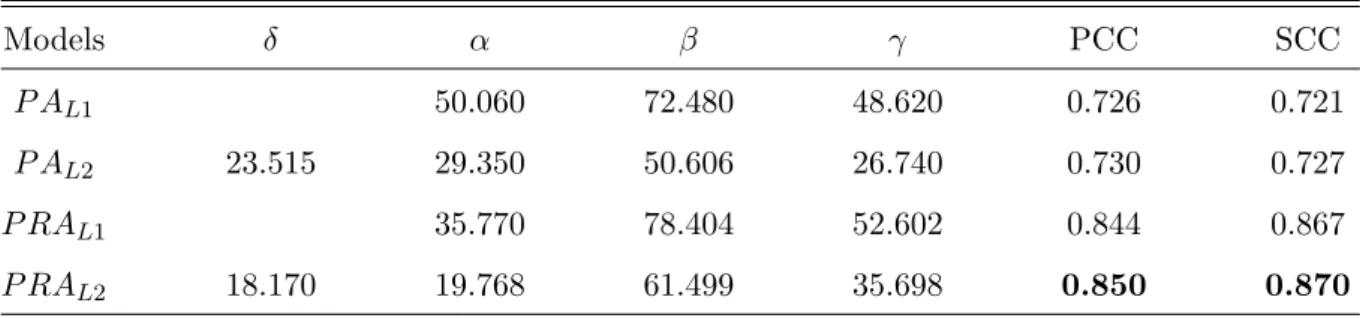
4.10 Fitting of the linear models to MAV and RMAV. . . 35

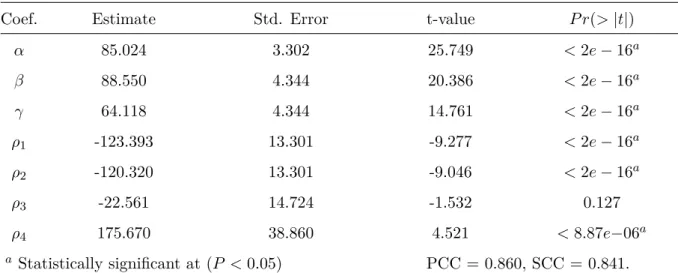
4.11 Fitting of the linear model with interactions (P AL3) to MAVs. . . 36

4.12 Fitting of the linear model with interactions (P AL4) to MAVs. . . 37

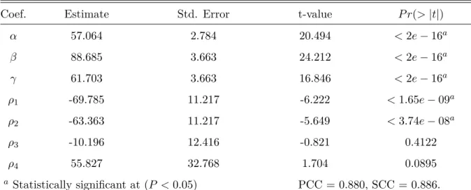
4.13 Fitting of the linear model with interactions (P RAL3) for RMAVs. . . 37

4.14 Fitting of the linear model with interactions and with an intercept coeﬃ-cient (P RAL4) for RMAVs. . . 38

4.15 Fitting of Minkowski models on MAV and RMAV. . . 38

4.16 Akaike Information Criterion for the linear and Minkowski models. A lower value indicates a better trade-oﬀ between model complexity and accuracy. . 40

4.17 Average correlation across the 10-fold cross-validation runs between model predictions and (R)MAVs . . . 40

5.1 Exp.1s: Pairwise comparisons between averageM SVpckwith diﬀerentPDP values for M = 12. (* Signiﬁcant at 0.05 level.) . . . 43

5.2 Exp.1s: Fitting parameters for linear model without intercept (P AE1,L1) (* Signiﬁcant at 0.05 level.) . . . 44

5.3 Exp.1s: Fitting parameters for linear model with intercept (P AE1,L2). (* Signiﬁcant at 0.05 level.) . . . 44

5.4 Pearson and Spearman correlation coeﬃcient of the linear models with and without intercept term, and SVR models on MAV. . . 44

5.5 Exp.2s: Pairwise comparisons between averageM SVblur for sequences with only-blurriness (*. Signiﬁcant at 0.05 level.) . . . 45

5.6 Exp.2s: Pairwise comparisons between averageM SVbloc for sequences with only-blockiness (*. Signiﬁcant at 0.05 level.) . . . 46

5.7 Exp.2s: Pairwise comparisons between average M SVbloc and M SVblur for any pair of blurriness and blockiness (*. Signiﬁcant at 0.05 level.) . . . 46

5.8 Exp.2s: Fitting parameters for linear model without intercept (P AE2,L1) (* Signiﬁcant at 0.05 level.) . . . 47

5.9 Exp.2s: Fitting parameters for linear model with intercept (P AE2,L2). (* Signiﬁcant at 0.05 level.) . . . 47

5.10 Exp.2s: Fitting parameters for the linear metric with interactions (P AE2,L3) (* Signiﬁcant at 0.05 level.) . . . 48

5.11 Exp.2s: Fitting parameters for the linear metric with interactions and in-tercept term (P AE2,L4). (* Signiﬁcant at 0.05 level.) . . . 48

(14)

5.13 Exp.2s: Fitting parameters for Minkowski model with intercept (P AE2,M2).

(* Signiﬁcant at 0.05 level.) . . . 49 5.14 Fitting of linear and non-linear models on MAV. . . 49 5.15 Exp.3s: Pairwise comparisons between average MSVs for sequences with

only -packet-loss, -blockiness, and -blurriness (*. Signiﬁcant at 0.05 level.) 50 5.16 Exp.3s: Pairwise comparisons between average MSVs for (PDP;blur)

se-quences (*. Signiﬁcant at 0.05 level.) . . . 51 5.17 Exp.3s: Pairwise comparisons between average MSVs for (PDP;bloc)

se-quences (*. Signiﬁcant at 0.05 level.) . . . 52 5.18 Exp. 3: Pairwise comparisons between average MSVs for sequences with

blockiness=0.4 and changing packet-loss and blurriness strengths (*. Sig-niﬁcant at 0.05 level.) . . . 53 5.19 Exp. 3: Pairwise comparisons between average MSVs for sequences with

bloc=0.6 and changing packet-loss and blurriness strengths (*. Signiﬁcant at 0.05 level.) . . . 54 5.20 Fitting parameters for linear model without intercept (P AE3,L1) (*

Signif-icant at 0.05 level.) . . . 54 5.21 Fitting parameters for linear model with intercept (P AE3,L2). (* Signiﬁcant

at 0.05 level.) . . . 54 5.22 Fitting parameters for the linear metric with interactions P AL3,E3 (*

Sig-niﬁcant at 0.05 level). . . 55 5.23 Fitting parameters for the linear metric with interactions and an intercept

term P AL3,E4 (* Signiﬁcant at 0.05 level). . . 56

5.24 Fitting parameters for the Minkowski modelP AL3,M1(* Signiﬁcant at 0.05

level). . . 56 5.25 Fitting parameters for SVR model by Experiments. . . 57 5.26 Akaike Information Criterion (AIC) for the linear and Minkowski models.

A lower value indicates a better trade-oﬀ between model complexity and accuracy. . . 58 5.27 Average correlation across the 10-fold cross-validation runs between model

predictions and MAVs . . . 58 5.28 Exp.1s: PCC, SCC, and AIC values obtained using a set of artifact metrics

to predict annoyance, with the linear models in Eqs. 5.1 and 5.2. . . 59 5.29 Exp.1s: PCC and SCC obtained usingBlocF andP ackRmetrics to predict

annoyance, with theP AE1,SV M model (SVR algorithm). . . 59 5.30 Exp.2s: PCC, SCC, and AIC values for the linear models considering all

(15)

5.31 Exp.2s: PCC, SCC, and AIC values for the linear models considering all NR artifact metrics for only-blurriness sequences. . . 60 5.32 Exp.2s: PCC, SCC, and AIC values for the linear models consideringBlocF

and BlurC. . . 61 5.33 Fitting parameters for the linear metric (P AE2,L4) with interactions, an

intercept term with BlocF and BlurC as parameters, for test sequences with only combination of blockiness and blurriness (* Signiﬁcant at 0.05 level). . . 61 5.34 Fitting parameters for the linear metric (P AE2,L4) considering all test

se-quences of Exp.2s, with BlocF and BlurC as parameters (* Signiﬁcant at 0.05 level). . . 62 5.35 Exp.3s: PCC, SCC, and AIC values for all model investigated. . . 62

7.1 Selectedfeatures ranked by importance. . . 84 7.2 Comparison of the correlation coeﬃcients computed from set of video databases

and artifact metrics. . . 85 7.3 Comparison of correlation coefficients per distortion in the CSIQ database. 86 7.4 Comparison of correlation coefficients per distortion in the LIVE database. 86 7.5 Comparison of correlation coefficients per distortion in the IVPL database. 87 7.6 Comparison of correlation coefficients per distortion in the Exp.1a database. 87 7.7 Comparison of correlation coefficients per distortion for Exp.2a database. . 88 7.8 Comparison of correlation coefficients per distortion in Exp.3a database. . 88 7.9 Comparison of the correlation coefficients computed from proposed metric

(PM) using MAV and RMAVs. . . 89 7.10 Comparison of the correlation coeﬃcients computed from P MRM AV and

(16)

Abbreviations

AIC Akaike Information Criterion. 24

FR Full-Reference. 10

HVS Human Visual System. 5

INLSA Iterative Nested Least Squares Algorithm. 35

ITU International Telecommunications Union. 8

M Frame Intervals. 19

MAV Mean Annoyance Value. 23

MSE Mean Square Error. 10

MSV Mean Strength Value. 23

NR No-Reference. 10

PCC Pearson correlation coeﬃcient. 23

PDP Percentages of Deleted Packets. 19

PSNR Peak Signal-to-Noise Error. 10

QoE Quality of Experience. 5

QoS Quality of Service. 5

RMANOVA Repeated-Measure ANOVA. 24

RR Reduced Reference. 10

(17)

SD Standard Deﬁnition. 4

SSIM Structural Similarity and Image Quality. 11

SVR Support Vector Regression. 6

UESL Upper Empirical Similarity Limit. 25

VQEG Video Quality Experts Group. 15

(18)

Chapter 1 Introduction

In modern digital imaging systems, the quality of the visual content can undergo a drastic decrease due to impairments introduced during capture, transmission, storage and/or display, as well as by any signal processing algorithm that may be applied to the content along the way (e.g. compression) [1, 2]. Impairments are deﬁned as visible defects (ﬂaws) and can be decomposed into a set of perceptual features calledartifacts [3]. The physical signals that produce the artifacts are known as artifact signals. Artifacts can be very complex in their physical and perceptual descriptions [4]. Being able to detect artifacts and reduce their strength can improve the quality of the visual content prior to its delivery to the user [5].

Generally, visual quality assessment methods can be divided into two categories: sub-jective and obsub-jective methods. Subsub-jective methods estimate the quality of a video by performing psychophysical experiments with human subjects [3]. They are considered the most reliable methods and are frequently used to provide ground truth quality scores. These methods also provide insights into mechanisms of the human visual system, in-spiring, not only the design of objective quality metrics, but of all kinds of multimedia applications [6]. Nevertheless, subjective methods are expensive, time-consuming and cannot be easily incorporated into an automatic quality of service control system. On the other hand, objective methods are algorithms (metrics) that aim to predict the visual quality. Objective metrics that take into account aspects of the human visual system usually have the best performance [7, 8], but are often computationally expensive and, therefore, hardly applicable in real-time applications [9].

(19)

metrics estimate impairment annoyance by comparing original and impaired videos [8,12]. Alternatives include artifact based metrics [13, 14], which estimate the strength of individual artifacts and, then, combine them to obtain an overall annoyance or quality model [14, 15]. The assumption here is that, instead of trying to estimate overall annoy-ance, it is easier to detect individual artifacts and estimate their strength because we ‘know’ their appearance and the type of process that generates them. These metrics have the advantage of being simple and not necessarily requiring the reference. They can be useful for post-processing algorithms, providing information about which artifacts need to be mitigated.

Naturally, the performance of an artifact based metric depends on the performance of the individual artifact metrics. Therefore, designing eﬃcient artifact metrics requires a good understanding of the perceptual characteristics of each artifact, as well as a knowl-edge of how each artifact contributes to the overall quality [14,16]. According to Moorthy and Bovik [8], little work has been done on studying and characterizing the individual artifacts [17–19].

For example, Fariaset al.[10,20] studied the appearance, annoyance, and detectability of common digital video compression spatial artifacts by measuring the strength and overall annoyance of these artifact signals, when presented alone or in combination in interlaced Standard Deﬁnition (SD) videos (480i). Their results showed that the presence of noisiness in videos seemed to decrease the perceived strength of other artifacts, while the addition of blurriness had the opposite eﬀect. Moore et al. [21] investigated the relationships among visibility, content importance, annoyance, and strength of spatial artifacts in interlaced SD videos. Their results showed that the artifacts’ annoyance are closely related to their visibility, but only weakly related to the video content.

Huynh-Thu and Ghanbari [22] examined the impact of spatio-temporal artifacts in video and their mutual interactions. They veriﬁed that spatial degradations aﬀected the perceived quality of temporal degradations (and vice-versa). Moreover, the contribution of spatial degradations to the quality is greater than the contribution of temporal degra-dations. Reibman et al. [23] showed that the temporal artifacts (e.g. packet-loss) have an important contribution to quality and can be successfully used to predict it.

(20)

propagation due to the motion-compensation loop.

Although a lot of work has been devoted in this study ﬁeld, currently there is no clear knowledge on how diﬀerent artifacts combine perceptually and how their impact depends on the physical properties of the video.

1.1 Problem Statement

The quality of a video may be altered in any of the several stages of a communication system (e.g. during compression, transmission and display). The quality of a video decreases when spatial1

or temporal2

artifacts are introduced [26]. It is worth pointing out that artifacts may also have spatial and temporal features, like for example packet-loss artifacts, which are a result of losses during the digital transmission [27].

Measuring the quality of a video is important for the design of communication systems that meet the minimum requirements of Quality of Service (QoS) and Quality of Expe-rience (QoE), therefore satisfying the end-user demands [7, 8]. Like mentioned earlier, quality must be estimated taking into consideration human perception (i.e. considering aspects that are considered relevant for the Human Visual System (HVS), such as color perception, contrast sensitivity etc.). For real-time applications, it is important to design quality metrics that are sufficiently fast and computationally efficient. It is worth men-tioning that, to design and validate a quality metric, it is important to compare its quality estimates with the subjective scores obtained by performing psychophysical experiments in which volunteers rate (using a predefined scale) the quality of a set of videos [26].

In the literature, most HSV-based metrics have the disadvantage of being computa-tionally complex and, many of them, require the reference at the measurement point. For these reasons, the use of these metrics in real-time applications is impractical [16]. One possible solution is to use feature extraction methods to analyze speciﬁc characteristics or attributes of the video or image (e.g. sharpness, blur, contrast, temporal ﬂuidity, arti-facts etc.) which are considered relevant to quality. A popular type of feature extraction metrics are artifact metrics, which estimate the strength of a set of artifacts considered perceptually relevant. These artifact strengths are then combined to obtain an estimate of the quality [14, 16].

Given that measuring video quality accurately and eﬃciently, without the use of hu-man subjects, is highly desirable [27], over the last twenty years a number of interesting

1_{Spatial artifacts are characterized by the presence of degradations that varying within the same frame} or image, such as blocking, blurring, noise, ringing etc.

(21)

techniques to estimate the overall video quality have been proposed [7,8,14,28,29]. Some proposals use specific functions (e.g. linear) to combine the results obtained from an analysis of common video distortions (e.g. coding and transmission artifacts) [6, 30]. For example, Farias et al. [14] proposed a set of artifact metrics that analyzed the strength of four types of artifacts and, then, combined their results to obtain the overall perceived annoyance. Their results presented a good correlation with subjective data. Wang et al. [31] designed a no-reference metric for JPEG compressed images that considered two type of artifacts: blockiness and blurriness. A non-linear model based on a power function was used to combine the measurements for each artifact. Given these previous results, we believe that a system composed of different artifact metrics, individually designed to assess the levels of degradation caused by specific artifacts, can be used to produce reliable quality estimates.

1.2 Proposed Approach

In this work, we have performed six psychophysical experiments, where participants were asked to detect the artifacts and rate their annoyance and the strength of artifacts. The artifacts were presented in isolation or in combination. The goal of that set of experiments was to try to understand how individual artifact perceptual strengths combine to produce the overall annoyance and to investigate the importance of each artifact while determining the overall annoyance in impaired videos.

So, we proposed a no-reference quality assessment method for estimating the quality of videos impaired with blockiness, blurriness, and packet-loss artifacts based in several

featuresextracted from de videos (e.g. DCT information, cross-correlation of sub-sampled images, average absolute diﬀerences between block image pixels, intensity variation be-tween neighbouring pixels, and visual attention). A non-linear regression model using Support Vector Regression (SVR) is used to combine all features to obtain an overall quality estimate. Our metric is an improvement of the techniques currently available in the literature and is designed with the requirement of not using the reference.

In summary, the main contributions of this work are:

1. A study of the visibility and annoyance of blockiness, blurriness, and packet-loss artifacts, presented in isolation or in combination;

2. An analysis of the perceptual contribution of these artifacts to the overall quality;

3. An analysis of the perceptual contribution of these artifacts to visual attention, and;

(22)

1.3 Organization of the Document

(23)

Chapter 2 General Aspects of Video Quality

In this chapter, we discussed the main aspects of subjective and objective quality assess-ment methods, describing the most common techniques, advantages, and drawbacks. We also brieﬂy described the processes that are responsible for the human visual attention and its relationship to video quality.

2.1 Subjective Quality Assessment Methods

The most accurate way to determine the quality of a video is by measuring it using jective quality assessment, i.e. psychophysical experiments performed with human sub-jects. The International Telecommunications Union (ITU) provides a set of experimental methodologies designed for image and video quality assessment. Recommendations ITU-T 930 [32] and IITU-TU-R BITU-T.500 [3] are the most commonly used standards for multimedia and broadcasting applications. These two documents describe settings for the physical environment and equipment, quality scoring methodologies, diﬀerent ways of presenting the stimuli, and statistical techniques that can be used to analyze the subjective data. Two of the most popular methodologies are the Single Stimulus (SS) and the Double Stimulus (DS) methods.

(24)

Stimu-Table 2.1: Quality Category Rating (QCR) and Degradation Category Rating (DCR) scales.

Quality Category Scale Degradation Category Scale

Category Score Category Score

Excellent 5 Imperceptible 5

Good 4 Perceptible, but not annoying 4

Fair 3 Slightly annoying 3

Poor 2 Annoying 2

Bad 1 Very annoying 1

lus Absolute Category Rating Scale (ACR-HRR), in which the (unprocessed) reference sequence is included in the experimental sessions without any identiﬁcation [33].

In the DS method, the test and reference sequences are presented simultaneously to the subject, who evaluates their quality by comparing them. Similar to the SS method, the evaluation can be performed for short or continuous sequences. The variations of the DS methodologies include Double Stimulus Impairment Scale (DSIS), Double Stimulus Continuous Quality Scale (DSCQS), and Simultaneous Double Stimulus for Continuous Evaluation (SDSCE).

The scales used in the experiments can have numbers (numeric scales) and/or ad-jectives (nominal scales). For example, in the Absolute Category Rating (ACR) scale participants rate the quality of test sequences using a scale with ﬁve adjectives with as-sociated numerical values. Concerning the type of perception being measured, when a Quality Category Rating (QCR) scale is used participants rate the video quality. Given that quality is an open ended scale (something of better or worse quality can always show up), experimenters often use a Degradation Category Rating (DCR) scale that allows participants to rate the intensity of the degradation, instead of the overall quality. Table 2.1 shows the QCR and DCR scales.

2.2 Objective Quality Assessment Methods

(25)

Depending on the amount of reference information required by the quality assessment algorithm, objective methods can be classiﬁed in three categories: Full-Reference (FR), Reduced Reference (RR), and No-Reference (NR) [7]. FR methods require the original and test (e.g. distorted) videos to estimate quality, while RR methods requires the test video and a description or a set of parameters from the original video. Finally, NR methods only require the test video.

Since FR methods require the reference, they can only be used in oﬀ-line applications or in encoder during compression process. Most of these methods quantity the error diﬀerence between reference and test videos. Two of the most famous FR methods are the Mean Square Error (MSE) and the Peak Signal-to-Noise Error (PSNR), which can be calculated using the following equations:

M SE = 1 N

N

X

i=0

(Ori−Dsi)

2

, (2.1)

P SN R= 10 log10

2552

M SE !

, (2.2)

where N is the total number of pixels in the video frame, Ori and Dsi are the ith pixels in the original and distorted video, respectively, and 255 is the maximum pixel intensity value.

Both PSNR and MSE have been widely used because of their physical signiﬁcance and simplicity, but over the years they have been widely criticized for not correlating well with the perceived quality measurement [35,36]. One reason for this is the fact that these metrics do not incorporate aspects of the human vision system in their computation. MSE and PSNR simply perform a pixel-to-pixel comparison, without considering the content or the relationship among the pixels. They also do not consider how spatial and frequency content are perceived by human observers [27]. An example as how these metrics do not correlate well with the perceived quality measurement is depicted in Figure 2.1, where PSNR values are the same for a set of images with diﬀerent impairments.

(26)

Naturally, the FR methods that have the best performance take into account the available human vision models. Nevertheless, they are often computationally complex and require a fine temporal and spatial alignment between the reference and distorted videos. Daly et al. [28] proposed a metric (visible differences predictor - VDP) which estimates the visible difference between a reference and test videos, taking into account the intensity of the light, spatial frequency, and the video content. Lubin et al. [38, 39] proposed a multiple-scale spatial vision model for estimating the probability of detecting artifacts by analyzing their color information and temporal variations.

Wang et al. [29] proposed an algorithm, Structural Similarity and Image Quality (SSIM), that takes advantage of the fact that human vision is highly adapted to scene structures. In other words, the algorithm compares the local pattern normalized pixel in-tensity with the luminance and contrast. The metric returns values between 0 and 1, with lower values corresponding to lower quality and higher values to higher quality. Pinson et al. [40] proposed a Video Quality Metric (VQM) that has been adopted by the American National Standards Institute (ANSI) as a standard for objective video quality metrics. VQM measures the strength of several kind of artifacts, such as blockiness, blurriness, etc.

As mentioned earlier, RR methods require only some information about the reference video. Frequently, this information is a set of features extracted from the original and sent over an auxiliary channel. RR methods can be less accurate than FR metrics, but they are less complex. Gunawanet al.[41] proposed an RR method that takes into account features of local harmonic strengths (LHS). LHS is calculated taking into account the harmonic gain and loss, which are obtained from a discriminative analysis obtained from gradient images. The harmonic intensity can be introduced as a spatial activity measurement estimated from the vertical and horizontal edges of the image. Other RR metrics include works of Carnec et al. [42], Voranet al. [43], and Wolf et al. [44].

NR methods are designed to blindly estimate the quality of a video. Therefore, NR are more adequate for broadcasting and multimedia applications, which often require a real-time computation. Nevertheless, the design of NR is a challenge and, although several works have been proposed in the literature [45–50], a lot work still needs to be done for these methods to become reliable. One popular approach in the design of NR methods are the feature-based methods or, more speciﬁcally, the artifact-based methods [15, 51]. These methods estimate the strength of individual artifacts and combine the results to obtain an overall annoyance (or quality) score [4, 16, 31, 52].

(27)

characteristics of each artifact, as well as the knowledge of how each artifact contributes to the overall quality [14, 16, 45, 46]. It is worth noting that most digital videos can be affected by several artifacts that relate to each other, what makes difficult to individually perceive these artifacts and obtain an estimate of the overall quality of the video as, for example, the effects of the simultaneous presence of several artifacts. The quality of a video affected by a combination of artifacts cannot be obtained by a simple linear combination of the estimated intensities of each type of artifact. Masking and other effects of interaction between artifacts may occur, making the prediction strategy more complex and dependent on the artifacts involved [27].

In our work, we considered the most traditional artifact metrics in the literature for estimating the strength of blockiness, blurriness, and packet-loss artifacts (see Table 2.2). Wang et al. [31] proposed a metric that estimates blockiness by taking the difference of pixel intensities across block boundaries. Vlachos [53] proposed a method that estimates blockiness by measuring the ratio between the correlation of intra- and inter-block pixels. The algorithm split the frame into 8×8 blocks and simultaneously sampled it in the ver-tical and horizontal directions, assuming that all visible blockiness artifacts have a visible corner. Farias et al. [14] modified the metric proposed by Vlachos [53]. They considered only one of the borders of the blocking structure and, instead of down-sampling the frame simultaneously, they split it into two separate parts (i.e. into vertical and horizontal directions). They claimed this modification improves the performance of the algorithm, although it slightly increases its complexity. These algorithms are computationally ef-ficient since they do not use complex transforms or require storing the entire image in memory.

Marziliano et al. [52] proposed a method that estimates blurriness by measuring the width of strong edges. Narverkar et al. [54] proposed a probabilistic framework that is based on the human sensitivity to blurriness in regions with different contrast levels. Crete et al. [55] proposed an approach that discriminates different (perceptible) levels of blurriness for the same image. In other words, their algorithm estimates quality by measuring the differences between a blurred image and its re-blurred version (higher intensity of blurriness).

(28)

Table 2.2: Artifact metrics by distortions.

Artifact metrics Artifact Alias

Babu [13] Packet-loss P ackB

Xia Rui [56] Packet-loss P ackR

Marziliano [52] Blurriness BlurM

Narverkar [54] Blurriness BlurN

Crete [55] Blurriness BlurC

Farias [14] Blockiness BlocF

Wang [46] Blockiness BlocW

2.3 Visual attention

Recent studies show that video quality is closely tied to gaze deployment [57]. When observing a scene, the human eye typically scans the video neglecting areas carrying little information, while focusing on visually important regions [58]. Wang et al. [59] showed that, within the ﬁrst 2,000ms of observation, gaze patterns target the main objects in a scene. Later, the gaze is redirected to other salient areas, yet not visually important. This result suggests that visual coding should be focused, at ﬁrst, into the main objects of the scene. Nevertheless, the presence of artifacts may disrupt natural gaze patterns, causing annoyance and, consequently, lower quality judgments [60]. Therefore, saliency information should be incorporated into the design of video quality metrics.

Research in the area of visual quality have focused on trying to incorporate gaze pat-tern information into the design of visual quality metrics [61], mostly using the assumption that visual distortions appearing in less salient areas might be less visible and, therefore, less annoying [62]. However, while some researchers report that the incorporation of gaze pattern information increases the performance of quality metrics, others report no or very little improvement [63]. One possible reason for such disagreement is that, still, the role played by visual attention in quality evaluation is unclear. Although it has been shown that, for images, artifacts in visually important regions are far more annoying than those in the background [64], it is still not clear if artifacts can create saliency (and therefore, attract gaze) on their own. And if so, it is unclear which type of artifacts can create saliency and at what perceptual strength. If artifacts can disrupt gaze patterns by creat-ing saliency, this should be taken into account in the design of quality metrics that make use of saliency or gaze pattern information. Unfortunately, the existing knowledge in this direction is scattered.

(29)

assessment tasks. They found that the quality task has a significant effect on the fixation duration, which increased on unimpaired images during a quality scoring task. Also, the type of impairment caused modifications in the gaze patterns. Redi et al. [60] analyzed the impact of three kinds of artifacts (JPEG compression, white noise and gaussian blur) and showed that they caused changes in the gaze patterns during both quality assessment and free-viewing tasks. Also, in Rediet al. [66] gaze pattern deviations were measured by analyzing similarities among saliency maps. They reported that the differences between the saliency maps (both for free-viewing and quality assessment tasks) seem to be more related to the strength of the artifacts impairing the images than to the type of artifacts. With respect to video, Le Meuret al.[67] examined the viewing behavior during quality assessment and free-viewing tasks. Differently from images, they found that the average fixation duration is almost the same for both tasks, whereas saliency does not change significantly when videos are impaired (coding artifacts). Redi et al. [68] investigated to what extent the presence of packet-loss artifacts influences viewing behavior. Contrary to Le Meur et al. [67], they found that saliency could significantly change from free-viewing to quality assessment tasks and that these changes were related to both video content and to packet-loss annoyance. Similarly, Mantel et al. [69] found a positive correlation between coding artifacts annoyance and fixation dispersion.

(30)

Chapter 3 Experimental Methodology

To understand the relationship between the perceptual strengths of blockiness, blurriness, and packet-loss artifacts and how they can be combined to estimate the overall annoyance, we performed a set of psychophysical experiments using test sequences with combinations of these artifacts at diﬀerent strengths [34]. The experiments shared identical experimen-tal methodology, interface, protocol, and viewing conditions. In this chapter, we detailed each experiment performed in this work.

3.1 Stimuli

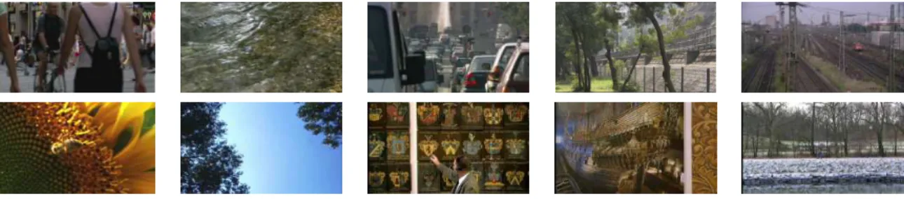
We used seven high deﬁnition original videos chosen with the goal of generating a diverse content. The videos have a spatial resolution of 1280×720 pixels, a temporal resolution of 50 frames per second (fps), and a duration of 10 seconds. Representative frames of each original are shown in Figure 3.1. We followed the recommendations detailed in the Final Report of Video Quality Experts Group (VQEG) on the validation of objective models multimedia quality assessment (Phase I) [72], which suggest to use a set of video sequences with a good distribution of spatial and temporal properties [73]. Figure 3.2 shows the spatial and temporal activity measures of the originals.

To add artifacts to the originals, we used a system for generating artifacts [20] that allowed a control of the artifact combination, visibility, and strength, which would be impossible when using, for example, a H.264 codec1

.

Packet-loss is a distortion caused by a complete loss of the packet being transmitted, without the error concealment algorithm (at the decoder) being able to recover the missing data. These artifacts are visually characterized by the presence of rectangular areas, whose content diﬀers from the content of the surrounding areas [68] (see Figure 3.3 (a)).

(31)

Figure 3.1: Frame videos. Top row: Park Joy. Middle row: Into Tree, Park Run, and Romeo and Juliet. Bottom row: Cactus, Basketball, and Barbecue.

Figure 3.2: Temporal and spatial information.

To generate packet-loss artifacts, we ﬁrst compressed the videos at high compression rates, what avoids inserting additional artifacts. Then, packets from the coded video bitstream were randomly deleted using diﬀerent loss percentages (the higher the percentage, the lower the quality) [34]. To vary the time interval between consecutive artifacts, we changed the number of frames between I-frames.

Blockiness is a distortion characterized by the appearance of the underlying block encoding structure, often caused by a coarse quantization of the spatial frequency com-ponents during compression [32] (see Figure 3.3 (b)). To add blockiness to each video frame in our dataset, we calculated the average value of each 8×8 block of the frame and of the 24×24 surrounding block, then added the diﬀerence between these two averages to the block.

(32)

(a) (b) (c)

Figure 3.3: A video frame with (a) packet-loss, (b) blockiness, and (c) blurriness artifacts.

blurriness, we used a simple low-pass filter, as suggested by Recommendation P.930 [32]. Although we can vary the filter sizes and the cut-off frequencies to control the amount of blurriness, we used a simple 5×5 moving average filter. We generated test sequences with combinations of blockiness and blurriness by linearly combining the original video with blockiness and blurriness artifact signals in different proportions (i.e. 0.4, 0.6, and 0.8) [75].

3.2 Methodology and Equipment

The experiments were performed using a PC computer with test sequences displayed on a Samsung LCD monitor of 23 inches (Sync Master XL2370HD) with resolution 1920×1080 @60hz (FullHD 1080p). The dynamic contrast of the monitor was turned oﬀ, the contrast was set at 100, and the brightness at 50. The monitor measured gamma values for luminance, red, green, and blue were 1.937, 1.566, 1.908, and 1.172, respectively. We set a constant illumination of approximately 70 lux. While watching the video sequences, the eye-movements were recorded using a SensoMotoric Instruments REDII Eye Tracker with a sampling rate of 50/60Hz. It has a pupil tracking resolution of 0.1◦ _{and a gaze position}

accuracy of 0.5 to 1. Participants were kept at a ﬁxed distance of 0.7 meters from the monitor using a chinrest. The experimental methodology was the single-stimulus with hidden reference, with a 100-point continuous-scale [3, 34].

The participants were mostly graduate students from UnB and Delft University. They were considered naive of most kinds of digital video defects and the associated terminology. No vision test was performed, but participants were asked to wear glasses or contact lenses if they needed them to watch TV. The experiment started after a brief oral introduction. The experiments were performed using the same experimental methodology. All exper-iments were divided into calibration, free-viewing, training, practice and an experimental session sessions:

(33)

data;

• Free viewing: participants were asked to freely look at seven high quality videos, as if they are watching TV at home;

• Training: participants were showed all four high quality videos. Then, videos with the strongest defect derived from each of the four high quality videos are shown. The intent of this stage is to familiarize the test participants with the endpoints of the annoyance scale and to clarify the experimental task;

• Practice: participants ran through a limited number of practice trials. The practice trials gives the participant a chance to work through the data entry procedure and shake out last minute questions or concerns. Also, since the initial responses may be somewhat erratic, the practice stage allows the test participant responses to stabilize. No data is collected during this task;

• Experimental Session: Participants are asked to watch several test sequences. After each sequence is played, the participant is asked: Did you perceive any im-pairments or defects in the video?, prompting for aYes orNoanswer. Then, partic-ipants are asked to perform an annoyance or a strength task. The annoyance task requires that the participant gives a numerical judgment of how annoying the de-tected impairment is. Impairments as annoying as those seen in the training session should be given a 100 annoyance score, sequences half as annoying a50 annoyance score, and so on. The strength task requires that the participant rate the strength of each artifact identiﬁed in the video. Artifacts as strong as those seen in the training session should be given a 100 strength score, sequences half as strong a 50

strength score, and so on. The number of artifacts present in the test sequences varied for each experiment. To avoid fatigue, the experimental session was broken into sub-sessions, between which participants could take a break for as long as they wanted to. All experimental sessions lasted between 45 and 60 minutes.

3.3 Subjective Experiments Details

In this section, we detail the experiments performed in this work.

3.3.1 Experiment 1

(34)

Table 3.1: Exp. 1: Combinations of the parameters PDP and M used for each of the 7 originals.

Comb M PDP Comb M PDP Comb M PDP

1 4 0.7 5 8 0.7 9 12 0.7

2 4 2.6 6 8 2.6 10 12 2.6

3 4 4.3 7 8 4.3 11 12 4.3

4 4 8.1 8 8 8.1 12 12 8.1

deleted packets from the coded video bitstream. The Percentages of Deleted Packets (PDP) used were 0.7%, 2.6%, 4.3%, and 8.1%. To vary the time interval between in-troduced artifacts, we varied the number of frames between the I-frames. Three Frame Intervals (M) were used: 4, 8 and 12. The set of PDP and M parameters used in the experiments are given in Table 3.1. A total of 7 originals and 12 parameter combinations were used, resulting in 12×7 + 7 = 91 test sequences. To avoid fatigue, these videos were evaluated in a single experimental session, divided in three sub-sessions with two 10-minutes breaks.

3.3.2 Experiment 2

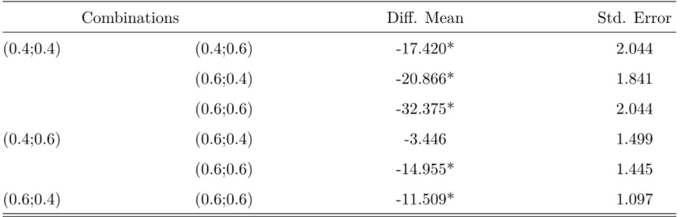
In this experiment, 16 participants rated annoyance (Exp.2a) whilst 15 participants per-formed strength tasks (Exp.2s) on test sequences containing diﬀerent strengths of block-iness and blurrblock-iness artifacts, presented in isolation or in combination. Strength combi-nations are represented by a vector (bloc; blur), where bloc is the blockiness strength and

blur is the blurriness strength. The experiments contained a set of videos with all possible combinations of the two artifact types at strengths 0.0, 0.4, and 0.6. Two additional com-binations, consisting of pure blockiness and pure blurriness at strength 0.8, were added to the experiments. Table 3.2 shows all combinations used in the experiments. A total of 7 originals and 10 combinations were used in this experiments, resulting in 10×7 + 7 = 77 test sequences.

3.3.3 Experiment 3

(35)

Table 3.2: Exp. 2: Set of combinations used for each of the 7 originals: bloc and blur

correspond to the blockiness and blurriness strengths, respectively.

Comb (bloc;blur) Comb (bloc;blur) Comb (bloc;blur)

1 (0.0;0.0) 5 (0.4;0.4) 9 (0.6;0.6)

2 (0.0;0.4) 6 (0.4;0.6) 10 (0.0;0.8)

3 (0.0;0.6) 7 (0.6;0.0) 11 (0.8;0.0)

4 (0.4;0.0) 8 (0.6;0.4)

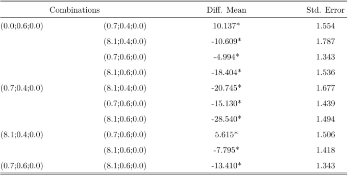
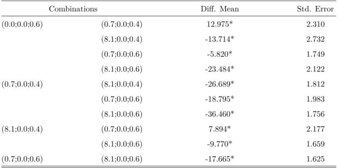
Table 3.3: Exp. 3: Combinations for each original: bloc corresponds to the blockiness strength, blur to the blurriness strength, and PDP to the packet-loss ratio.

Comb. (PDP;Bloc;Blur) Comb. (PDP;Bloc;Blur) Comb. (PDP;Bloc;Blur)

1 (0.0;0.0;0.0) 8 (8.1;0.0;0.6) 15 (0.7;0.6;0.0)

2 (0.0;0.6;0.0) 9 (0.7;0.4;0.0) 16 (8.1;0.6;0.0)

3 (0.0;0.0;0.6) 10 (8.1;0.4;0.0) 17 (0.7;0.6;0.4)

4 (8.1;0.0;0.0) 11 (0.7;0.4;0.4) 18 (8.1;0.6;0.4)

5 (0.7;0.0;0.4) 12 (8.1;0.4;0.4) 19 (0.7;0.6;0.6)

6 (8.1;0.0;0.4) 13 (0.7;0.4;0.6) 20 (8.1;0.6;0.6)

7 (0.7;0.0;0.6) 14 (8.1;0.4;0.6)

(36)

3.4

3.4.1 Image and Video Processing Laboratory (IVPL)

The IVPL database was developed at the Chinese University of Hong Kong. It contains 10 pristine videos and 4 types of distortions: MPEG2 compression (MPEG2), Dirac wavelet compression (Dirac), H.264 compression (H264), and packet-loss on the H.264 streaming through IP networks (IP). In this work, we have only used sequences with H264, MPEG2, and IP distortions. All videos are in raw YUV420 format, with a spatial resolution of 1920×1088 pixels, duration of 10 seconds, and a temporal resolution of 25fps. Each video was rated by 42 participants in a single-stimulus quality scale test method (ACR). Figure 3.4 shows a frame of each original video of the IVPL database.

Figure 3.4: Sample images of source video contents from IVPL database.

3.4.2 Laboratory for Image & Video Engineering (LIVE)

(37)

Figure 3.5: Sample images of source video contents from LIVE database.

hidden reference removal. Participants scored the video quality on a continuous quality scale. Figure 3.5 shows a frame of each video used in our tests.

3.4.3 Computational and Subjective Image Quality (CSIQ)

The CSIQ video database was developed to provide a useful dataset for the validation of objective video quality assessment algorithms. It consists of 12 high-quality reference videos and 216 distorted videos, containing six types of distortion at three diﬀerent levels of distortion. The distortion types consist of four compression-based distortion types and two transmission-based distortion types, such as H.264 compression (H264), HEVC/H.265 compression (HEVC), Motion JPEG compression (MJPEG), Wavelet-based compression using the Snow codec (SNOW), H.264 videos subjected to simulated wireless transmission loss (Wireless), and Additive white noise (AWGN). However, in this work, we have only used the sequences with H264, Wireless, MJPEG, and HEVC distortions. All the videos are in the YUV420 format, with a spatial resolution of 832 × 480, a duration of 10 seconds, and temporal resolutions ranging from 24 to 60 fps. Each video was assessed by 35 participants following the SAMVIQ methodology. Figure 3.6 shows a frame of each video used in our tests.

(38)

3.5 Statistical Analysis

Data gathered from the six experiments provided up to four diﬀerent results for each test sequence: Eye-tracker data, Mean Annoyance Value (MAV), Mean Strength Value (MSV) and, Probability of detection (Pdet). Also, the MSV values were divided inM SVbloc, M SVblur, and M SVpck, which correspond to MSVs for blockiness, blurriness, and packet-loss, respectively.

To analyze the subjects’ data gathered during detection tasks, we ﬁrst converted the

yes/noanswers to binary scores, such as,yeswas saved as 1, whilenowas saved as 0. The Pdet an impairment is, then, estimated by counting the number of subjects who detect this impairment and dividing by the total number of subjects.

MAVs are computed by averaging the annoyance values over all participants, for each video:

M AV = 1 S

S

X

i=1

A(i), (3.1)

where A(i) is the annoyance value reported by the ith _{participant and,} _S _{is the number} of human subjects.

MSVs are computed by averaging the strength values over all participants, for each video and artifact type:

M SV = 1 S

S

X

i=1

S(i), (3.2)

where S(i) is the strength value reported by the ith _{participant and,} _S _{is the number} of human subjects. The MSV is computed for each type of artifact, i.e. blockiness, blurriness, or packed-loss. To study how the artifact strengths combine to predict the perceived annoyance of videos impaired by multiple and overlapping artifacts, we ﬁt a set of linear and non-linear models to the MSV subjective data and the MAV data collected for the same test sequences [34, 79].

(39)

We use the Akaike Information Criterion (AIC) [80] to analyze the trade-off between fitting accuracy and the number of degrees of freedom of the model, thereby controlling for the bias/variance trade-off and over-fitting. To test the effect of the artifact parameters on annoyance, we performed a Repeated-Measure ANOVA (RMANOVA) with a significance level of 95% (α= 0.05).

Finally, we used a SVR algorithm to predict annoyance from the subjective data. The SVR algorithm is used to combine all features extracted from de videos impaired with blockiness, blurriness, and packet-loss. To train the SVR, we used ak-fold cross validation setup, i.e. we split the dataset ink equally sized non-overlapping sets and ran the training k times (with k equal 10). Each time, we use a diﬀerent fold as test set, while using the remaining k−1 folds for training [81].

3.6 Analysis of eye-tracking data and quality scores

To investigate the impact of the presence of multiple artifacts on users gaze patterns, we tracked eye-movements of participants during the psychophysical experiments (i.e. Exp.3a). Therefore, experiments produced two types of output: eye-tracking data and subjective scores. For both outputs, we had one recording per participant and per video content. The subjective scores collected for each video sequence were averaged over par-ticipants, as described in the previous section.

The eye-tracking data consisted of pupil movements, recorded in terms of fixation points and saccades. However, we limited ourselves to the analysis of fixation data, which is considered to be one of the most informative data regarding viewing behavior. Specifically, we analyzed viewing behavior by looking at two quantities: the duration of the fixations, found to be impacted by quality scoring in Ninassi et al. [65], and the spatial deployment of gaze patterns. We quantified the latter via saliency maps [82] which represent, per each video pixel, the probability that it will be gazed at by an average observer. This choice is in line with most of the existing literature in the area [61].

(40)

a Gaussian patch with width equal to approximately the fovea size (2◦ _{visual angle). This}

procedure was applied for each video sequence, creating 10,000

400 ms= 25 saliency maps per

video content. For the sake of analysis, the saliency maps are clustered into the following groups:

1. F VP V corresponding to pristine videos, captured during the free-viewing task;

2. SCP V corresponding to pristine videos, captured during the quality assessment task;

3. SCG1 corresponding to test sequences with artifacts in isolation (Combinations 2 to

4 in Table 3.3), captured during the quality assessment task;

4. SCG2 corresponding to test sequences with combinations of two artifacts

(Combi-nations 5 to 12 in Table 3.3), captured during the quality assessment task;

5. SCG3 corresponding to test sequences with combinations of three artifacts

(Combi-nations 13 to 20 in Table 3.3), captured during the quality assessment task.

Finally, we analysed if viewing behavior changes across these ﬁve groups from two inde-pendent variables: task (free-viewing or quality assessment) and degradation (pristine or impaired). For impaired videos, we also were interested in checking whether the number and/or type of artifacts impact the saliency maps and the ﬁxation durations.

3.6.1 Similarity measures for detecting saliency changes

Similarity measures are used as indicators of changes in saliency distribution and therefore in gaze patterns [66, 83]. The following measures were adopted to estimate the extent to which saliency maps corresponding to a certain time window of a certain video changes across the groups indicated above.

1. Linear correlation coeﬃcient (LCC) ∈ [1 -1], which quantiﬁes the strength of the linear relationship between two saliency maps.

2. Structure Similarity Index (SSIM [29])∈ [0 1], which indicates the extent to which the structural information of a map is preserved in relation to another map.

In both similarity measures, a value close to 1 indicates high similarity, while a value of 0 indicates dissimilarity, in turn suggesting a consistent change in the image saliency and consequently of the spatial allocation of gaze.

(41)

video, at the same level of impairment, and under the same task), but for two diﬀerent groups of participants. As such, it expresses the extent to which two saliency maps are similar given individual diﬀerences in participants. UESL represents an useful benchmark to understand whether dissimilarity in maps, as measured after a change in experimental conditions (e.g. between a free-viewing map and a quality assessment map), is due to inter-subject variability rather than to the change in experimental conditions. We calculated UESL based on LCC using with the following equation:

U ESL(LCC, vi) = 1 T

T

X

t=1

LCCSMvF VP V0

i,t

, SMvF LP V1

i,t

, (3.3)

where SM(vF L

i,t ) indicates the saliency map computed for time slot t, video vi, F V is the observer group, and T is the total number of ﬁxations over all observers. The saliency maps SM(vF VP V0

i,t ) were recorded in our experiments from the pristine videos during the free-viewing task (F VP V). The saliency maps SM(v

F VP V1

(42)

Chapter 4 Annoyance Models

Understanding the perceptual impact of compression artifacts in video is one of the keys for designing better coding schemes and appropriate visual quality control chains. Al-though compression and transmission artifacts, such as blockiness, blurriness and packet-loss, appear simultaneously in digital videos, traditionally they have been studied in iso-lation. In this chapter, we reported the analysis of the annoyance tasks performed in the three subjective experiments (i.e. Exp.1a, Exp.2a, and Exp.3a). Our goal here is to study the perceptual characteristics of a set of artifacts common in digital videos (blockiness, blurriness and packet-loss), presented in isolation and in combinations. Based on this analysis, we designed several annoyance models for videos degraded with these artifacts.

4.1 Introduction

Based on the results of three psychophysical experiments, we investigated how spatial and temporal artifacts combine to determine quality [68, 84] by measuring the annoyance and detection characteristics of two spatial artifacts (blockiness and blurriness) and a very important temporal artifact (packet-loss). Up to our knowledge, there is no study in the literature that performs an analysis of the inﬂuence spatial-temporal artifacts (in isolation and in combinations) have on the perceived annoyance. Most importantly, there is no study on how spatial and temporal artifacts interact to produce overall annoyance. To quantify the contribution of each artifact to the overall annoyance and of the interactions among the diﬀerent artifacts, we tested linear and non-linear annoyance models.

4.2 Experiment 1: Packet-Loss

(43)

Figure 4.1: Exp.1a: Average MAV plots for diﬀerent values of PDP: 0.7%, 2.6%, 4.3% and 8.1%.

Into Tree and Barbecue). This means that, for these two videos, all participants saw impairments in all test cases. It is worth pointing out that these two scenes have large smooth regions (e.g. skies) that make impairments easier to detect. Park Joy, Cactus, and Basketball have values of Pdet that grow (and saturate) very fast as MSE increases. On the other hand, Pdet for Park Run and Romeo and Juliet increases at a slower rate. This indicates that, for these scenes, it is harder to detect packet-loss artifacts. Romeo and Juliet, although having small spatial and temporal activity, is relatively dark and has a very clear focus of attention (the couple). On the other hand, Park Run has lots of spatial and temporal activity and not a lot of camera movement (see Figure 3.2). All of this makes it harder to spot packet-loss artifacts.

Next, we analyzed the influence of M and PDP on MAV. Figure 4.1 shows a plot of the average MAVs for the three values of M and the four values of PDP. Notice that MAV increases with bothPDP andM, butPDP has a bigger effect on MAV thanM. The effect of PDP on MAV is clearly significant. We performed a RM-ANOVA for analyzing the influence of M on MAV. Table 4.1 shows the pairwise comparisons between average MAVs for different M parameters. Notice that there are significant statistical differences between average MAVs for any pair of M values, except for the pair M = 4 and M = 8 for PDP=0.7%.

4.3 Experiment 2: Blockiness and Blurriness

(44)

Table 4.1: Exp.1a: Pairwise comparisons between average MAVs for diﬀerent M values. (* Signiﬁcant at 0.05 level. )

M values Diff. Mean Std. Error

4 8 -0.170 1.512

4 12 -9.134* 1.664

8 12 -8.964* 1.946

(a) (b) (c)

Figure 4.2: Exp.2a: Average MAVs for: (a) blurriness, (b) blockiness, and (c) combina-tions of blockiness and blurriness.

Pdetvalues got lower MAVs, while test sequences with higherPdet values got higher MAVs. Figures 4.2 (a) and (b) show plots of the average MAVs for sequences with only blockiness and blurriness, respectively, at strengths 0.4, 0.6, and 0.8. As expected, average MAVs increase with the artifact strength.

A RM-ANOVA was performed to check if MAV differences for different blockiness and blurriness strengths are significant. Table 4.2 displays the results, showing that there are significant statistical differences in MAV for all pairs of different strengths in only-blockiness and only-blurriness sequences.

Table 4.2: Exp.2a: Pairwise comparisons of MAVs for videos with only blockiness ( ˆF = 85.62, α≤0.01) and only blurriness ( ˆF = 334.75, α≤0.01). (* Signiﬁcant at 0.05 level)

Blockiness Blurriness

Strengths Diff. Mean Std. Error Diff. Mean Std. Error

0.4 0.6 -22.982* 1.863 -22.295* 2.796

0.8 -33.125* 3.179 -66.107* 2.526

No-reference Video Quality Assessment Model Based on Artifact Metrics for Digital Transmission Applications

Universidade de Brasília

No-reference Video Quality Assessment Model Based

on Artifact Metrics for Digital Transmission

Applications

Alexandre Fieno da Silva

Universidade de Brasília

No-reference Video Quality Assessment Model Based

on Artifact Metrics for Digital Transmission

Applications

Alexandre Fieno da Silva

Acknowledgements

Resumo

Abstract

Contents

List of Figures

List of Tables

Abbreviations

Chapter 1

Introduction

1.1

Problem Statement

1.2

Proposed Approach

1.3

Organization of the Document

Chapter 2

General Aspects of Video Quality

2.1

Subjective Quality Assessment Methods

2.2

Objective Quality Assessment Methods

2.3

Visual attention

Chapter 3

Experimental Methodology

3.1

Stimuli

3.2

Methodology and Equipment

3.3

Subjective Experiments Details

3.3.1

Experiment 1

3.3.2

Experiment 2

3.3.3

Experiment 3

3.4

Other Video Databases

3.4.1

Image and Video Processing Laboratory (IVPL)

3.4.2

Laboratory for Image & Video Engineering (LIVE)

3.4.3

Computational and Subjective Image Quality (CSIQ)

3.5

Statistical Analysis

3.6

Analysis of eye-tracking data and quality scores

3.6.1

Similarity measures for detecting saliency changes

Chapter 4

Annoyance Models

4.1

Introduction

4.2

Experiment 1: Packet-Loss

4.3

Experiment 2: Blockiness and Blurriness