Direct block scheduling under marketing uncertainties

(1)

275

Abstract

Mineral projects are composed of geological, operational and market uncertain-ties, and reducing these uncertainties is one of the objectives of engineering. Most surveys assess the impact of geological and operational uncertainties on the mining planning. The objective of this work is to study the impact of market uncertainty on the mineral activity. The influence of iron ore price simulation on mining sequencing will be evaluated. The price of iron ore has random behavior that is best represented by the Geometric Brownian Movement system. This study analyzed the historical series of iron ore in order to determine the percentage volatility and drift. Traditionally, a constant and deterministic price is used for the ore mined in all periods of a mineral project. The direct block scheduling methodology was adopted because it is able to apply the appropriate financial discount factor to the simulated probabilistic price. The proposed methodology was able to quantify the market uncertainty.

Keywords: mine planning, mine scheduling, direct block scheduling, price simulation, Brownian motion.

Hudson Rodrigues Burgarelli Mestrando

Universidade Federal de Minas Gerais – UFMG Escola de Engenharia

Departamento de Engenharia de Minas Belo Horizonte – Minas Gerais – Brasil hburgarelli@gmail.com

Felipe Ribeiro Souza Professor

Universidade Federal do Mato Grosso – UFMT Instituto de Engenharia

Várzea Grande – Mato Grosso – Brasil felipersminas@yahoo.com.br Alizeibek Saleimen Nader Professor

Departamento de Engenharia de Minas Belo Horizonte – Minas Gerais – Brasil beckn@demin.ufmg.br, beckn@usp.br Vidal Félix Navarro Torres Pesquisador

Instituto Tecnológico Vale Ouro Preto – Minas Gerais – Brasil lavra.itv@itv.org, vidal.torres@itv.org Taís Renata Câmara

Pesquisadora

Instituto Tecnológico Vale Ouro Preto – Minas Gerais – Brasil tais.camara@itv.org

Carlos Enrique Arroyo Ortiz Professor

Departamento de Engenharia de Minas Belo Horizonte – Minas Gerais – Brasil carroyo@demin.ufmg.br

Roberto Galery Professor

Departamento de Engenharia de Minas Belo Horizonte – Minas Gerais – Brasil rgalery@demin.ufmg.br

Direct block scheduling

under marketing uncertainties

Mining

_Mineração

(2)

Max

P_t=i

[

Part 1 - Part 2 + Part 3 - Part 4

]

Part 1 =

N_t=1

E

{NPV

_it

}

b

t i

Part 2 =

U

j=1

E

{NPV

t j

+ MC

}

W

Part 3 =

M_S=1

E

_{

SV M

t

{

K

tS

Part 4 =

M S=1

{

C

to

_d

to

_{+ C}

to

_d

to

_{+ C}

tg

_d

tg

₊

_C

tg

_d

tg

_{+ C}

tq

_d

tq

_{+ C}

tq

_d

tq

_}

u su l sl u su l sl u su l sl

1. Introduction

The methodology based on Lerchs-Grossmann and deterministic pricing can be considered the standard methodology adopted by the industry (SME, 2011). Due to the global need for greater reliability in the planning of mineral projects, direct block scheduling is considered the most adequate methodology (Souza, 2016). Direct block sequencing (SDB) is able to determine the destination of the block using the appropriate discount factor for the period in which it will be mined. Ideally the SDB should be able to use the simulated product price to apply the cor-rect discount factor (Dimitrakopoulos, 2011). The present study begins with a concise and thorough review of SDB formulation to demonstrate that it is able

to apply the financial discount factor correctly in order to mine the blocks of greater market uncertainty at the end of the mine life (Spleit, 2014). The price was simulated using the Geometric Brownian Motion. The proposed revision focuses on the sequential process, that is, the ability to generate the price at a time t according to the value contained in time t-1. It is impor-tant to consider that percentage volatility and drift; that is, the trend of the simula-tion is determined by historical values. The currently available system is not able to apply the correct discount factor and use the simulated price simultaneously. To use the simulated price, a two-stage methodology was developed. The first stage uses SDB to generate an initial

solu-tion with a correct discount factor, but with deterministic and constant price. This step determines in which period each block will be mined. With this informa-tion, it is possible to recalculate the benefit function considering the simulated price for the period in which the block will be mined. The second step begins with the use of the SDB with the benefit function of the blocks recalculated according to the simulated price. The second stage must be performed recursively until the stabi-lization of the mining period is achieved. The greatest contribution of this work is joining price simulation and direct block scheduling. Direct block scheduling is able to rearrange all sequencing due to change of one parameter or value in one block.

Direct block scheduling

The mining planning process can be divided briefly into the follow-ing steps: final pit definition with the generation of nested pits, pushback or mining phase definition for each period, including blending and cut-off grade optimization, and stock piles creation.

The traditional methodology can be enhanced with the adoption of a single optimization process, called Direct Block Scheduling or Block by Block. The direct block sequencing evaluates each block individually, while the classical method-ology evaluates the viability of the graph

for the decision to mine the set of blocks (Souza et al, 2014). This methodology considers all models simulated simulta-neously within an optimization process that returns a single mining sequence. Almeida (2013) presents a formulation of the problem:

P: periods number;

b_it_{: block}_i_{mined in period}_t_{and processed}

in the same period;

N: total number of blocks;

w_jt_:_block_j_{mined in period}_t_{and sent to}

the stockpile;

MC_jt_:_{cost to send the block}_j_{to the stockpile,}

in the period t;

U: nu mb er of blo ck s c on sidere d

for stockpiling;

k_st_:_block_s_{processed from the stockpile}

dur-ing period t.

SV t_:_{profit per tonne generated;}

M: number of simulated models

d_sut-_:_{risk quantified by the excess in ore}

pro-duction, grade and metal propro-duction, over

each scenario s;

d_slt-_:_{risk quantified by the deficiency in ore}

production, grade and metal production, over each scenario s;

C_ut-_:_{penalty cost associated to the excess in}

ore production, grade and metal production;

C_lt-_:_{penalty cost associated to the deficiency in}

ore production, grade and metal production;

(1)

Brownian motion

Brownian motion represents the zig-zagging motion exhibited by a particle, such as a grain of dusty fallen in a liquid or a gas. Small swings in commodity price and financial indicator charts resemble this movement. The financial market uses

Brownian motion to model the commod-ity price behavior. These models have more adherence and importance when related to short-term models. Due to the nature of the system, which considers that the random walk has a greater tendency

to short term variability, the system has a higher reliability in a shorter period (Rah-manpour & Osanloo, 2015). The process is classified as a Brownian motion if it is able to comply with the condition derived from the stochastic differential equation:

dS

_t

= µ

S

_t

d

_t

+

σ

S

_t

dW

_t (2) St= Simulated Solution;

µ= percentage volatility;

σ= percentage drift;

(3)

277

Using the market interest rate as a control factor of the simulations variance, 20 simulation scenarios

were generated for 10 years, based on the history of the iron ore prices. The beginning of the simulation considered

the year 2010 because it would be pos-sible to validate the scenarios generated with the reality.

2. Materials and methods

The objective of this paper is to dem-onstrate the methodology created to join the

probabilistic price simulation and the correct application of the discount factor in the mine

sequence. The procedures were divided into price simulation and mining sequencing.

Price simulation

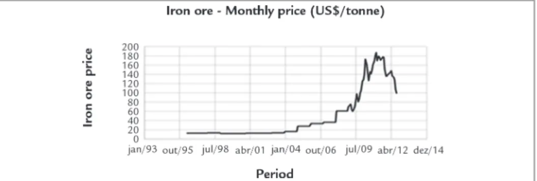
To determine what simulation model would be used, a consistent price history was required. The site indexmundi.com provided the historical series of iron ore prices from July 96 to September 2012. It

was concluded that there are tendencies to regionalized randomization that compose a global trend. This phenomenon can be observed in Figure 1, where we have a se-quence of small local noises that make up

for the global trend of price ascendance or descent. According to the trend of global and local oscillation, it was decided to use the Geometric Brownian Movement (Rahmanpour & Osanloo, 2015).

Figure 1 Iron ore price history.

For the determination of the variables μ and σ present in equation 1, it was used linear regression of the experimental data to the theoretical modeling. The average reversal process generates different values considering

all the values or only the descending price process started in April 2010. Considering all the values implies that there is a trend of price growth; however, considering prices from April 2010 to the end of the series implies a

downward trend. As the current eco-nomic downturn continues, the price decay fraction will be used to simulate future prices. The parameters used in the Geometric Brownian Motion are presented on Table 1:

MODEL PERCENTAGE VOLATILITY PERCENTAGE DRIFT

All Series 4.8076 0.0510

Final Fraction 5.1868 0.0335

Table 1 Parameters of Geometric Brownian Motion.

For the experiment, the price series called "Final Fraction" was selected due to

the greater adherence to the current real-ity of the iron ore market. The geometric

Brownian motion formulation was used to generate 20 different price scenarios.

Figure 2 Selling prices simulations.

It is possible to note in Figure 2 that there is a curve showing a growth tendency, while all other simulations show a decreasing tendency. This discrepant curve is the result of the interaction of several growth extreme

points of the probability histogram. Most simulations tend to follow the average, but there is always a prob-ability that one curve will result in few extreme scenarios. The influence of macroeconomic factors can affect

(4)

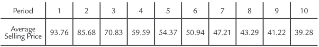
Period 1 2 3 4 5 6 7 8 9 10 Average

Selling Price 93.76 85.68 70.83 59.59 54.37 50.94 47.21 43.29 41.22 39.28 Table 2

Average selling prices.

Mining sequence first step

The first step is to determine the deterministic mining sequence for the constant price of 58.62US $/t. Constant selling price was calculated from the av-erage of all the simulations in all periods (58.62 US$/t). Trocar para “The average

selling price (Table 2) was calculated from the average of the simulations, for each of the 10 periods. The study was conducted in a real iron ore deposit, located in the “Quadrilátero Ferrífero”, an area in Brazil with high incidence

of iron ore deposits. The objective is to verify the impact of the price oscillation in the mining sequencing considering long term. The parameters used in the optimization process are presented on Table 3:

Parameter Value

Dilution 0%

Mine recovery 100%

Sales Price According Simulation

Mine Cost(Ore and Waste) 1.49 US$/t

Administrative Cost 0.59 US$/t

Process Cost 2.27 US$/t

Sales Cost 17.73 US$/t (Product)

Production Target 40 Mt ROM / Year

Discount Factor 5 % Year Table 3

Optimization parameters.

The result is a mining sequence generated for deterministic data. This

de-terministic block model with the defined mine periods will be used in the next step.

Mining sequence second step

This step uses the sequenced block model generated in the previous step. Each block has a benefit function calculated in the deterministic

sequenc-ing. The probabilistic SDB requires that each possible realization for the block has a specific value, so each block has 10 possible values according to the

simulated price. Equations 3, 4 and 5 show how the simulated price affects the benefit function.

Benefit Function[i,p] = Block Value[i] – Block Costs

Block Value[i,p] = Recovered Material x Simulated Price[i,p]

Block Cost = Mined Material x Sum of Costs

(4) (3)

(5)

The first step has the objective of determining an initial mine period, so the benefit function will be calculated based on this mine period for each of the 20 simulations. Benefit function will be updated continuously, using simulated prices. In other words, the benefit func-tion of the blocks flagged to be mined in period t will be updated with the simu-lated sales prices for this same period.

After updating the benefit function of all blocks, a new mining schedule sce-nario will be generated. This recursive step must be performed several times in order to generate various scenarios and to evaluate the system convergence. The second step can be called the recursive step, because several cycles must be performed until the block exchange sta-bilization. For the first round 58.62US

$/t price was used and this first round will generate the basic scheduling. After the first round is completed, it is possible to know in which period each block will be mined. After this round, it will be possible to join the simulated prices with the direct sequencing of the blocks. The benefit function has been updated according to the value of the simulated price according to Table 2.

i= Simulation Number; p=period mined.

3. Results and discussion

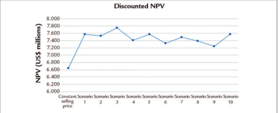
This process was carried out 10 times, generating 10 different scenarios, in order to try to understand the impact of this change in the mining sequence. Figure 3 shows that the values oscillate

around 7,400 US$ Million for NPV. Convergence demonstrates that higher and lower price scenarios forced the SDB algorithm to determine different sequencing that led to similar value

(5)

279 Figure 3

Discounted NPV for the mine schedule results.

In all cases with variable selling prices, there was a gain in the dis-counted NPV, when compared with the mining sequence generated with a constant selling price. It is noticed

that among the 10 scenarios analyzed, the NPV had a variation, but always around the same average. It is im-portant to analyze the changes in the decision of the blocks mining period.

The percentage of blocks that had the mining period changed in each scenario were analyzed, considering the previous scenario. The results are presented on Table 4:

Percentage

Scenario 1

Scenario 2

Scenario 3

Scenario 4

Scenario 5

Scenario 6

Scenario 7

Scenario 8

Scenario 9

Scenario 10

53.5 55.2 46.1 60.8 52.3 57.2 45.5 52.9 56.7 53.1

Table 4

Percentage of blocks with change in the mining period.

In the scenarios with variable selling price, simulated models were used, allowing

the quantification of the uncertainty of these mining sequences, regarding the sale price.

Figure 4 shows the Scenario 10 NPV results, associated with the price uncertainty:

Figure 4 NPV Scenario 10.

Figure 5 Loss probability.

The chart analysis shows that there is a probability that the last 4 years of the mining sequence presents a negative NPV. The maximum value

presented is very high, and it was caused by the discrepant curve with growth tendency. This curve is a result of the simulation process and is not due to

(6)

4. Conclusions

With the proposed methodology, combined with the Direct Block Scheduling, it was possible to analyze the impact of the selling price variation over time in the mine sequencing. It is possible to notice in Figure 3 that simulated prices have similar NPV levels. The simulated scenarios have an NPV greater than the deterministic scenario, ap-proximately 13%, due to the lower price in the final periods, forcing the system to be eager for rich blocks in the first periods. The results showed that this variation might affect the mining period of a great number of blocks, thereby altering the NPV of the mining sequence. In all scenarios there was a significant change in the mining period of the blocks. It was possible to generate various scenarios with higher NPV and

furthermore, quantify the uncertainty as-sociated to each scenario. Additional stud-ies can be performed to verify if the results obtained in this method will converge to a result, when performing a large number of iterations. Ideally, the Direct Block Schedul-ing system should incorporate this variation in the generation of the mining sequences, but this would considerably increase the complexity of the problem. The method-ology presented is capable of quantifying market risk. Figures 4 and 5 shows that it is important to pay all investments before year 7, as Figure 5 shows that there is a real prob-ability of the enterprise generating negative cash flow values. Analyzing Figures 2 and 4 allows us to conclude the importance of considering the extreme values of economic

scenarios generated by geometric Brownian motion, as there is always the possibility that external macroeconomic factors raise the prices of commodities, for example, a war. The accounting of the extreme price scenario triggered, in Figure 4, a remote pos-sibility of high present value that may occur although unlikely. Finally, the assertiveness of the selling price simulations should be analyzed, because as demonstrated, this parameter can significantly affect the mining sequence. The responsible engineer should always take the decision of which mining sequence must be adopted, but the new developed methodologies are impor-tant, providing a better understanding of the variables and uncertainties involved in the process.

References

ALMEIDA, A. M. Surface constrained stochastic life-of-mine production schedulling. Canada: McGill University, 2013. (Master of Engineering Thesis)

DIMITRAKOPOULOS, R. Stochastic optimization for strategic mine planning: A de-cade of developments. Journal of Mining Science, v. 47, n. 2, p. 138-150, 2001, DOI: 10.1134/S1062739147020018

ELKINGTON, T., DURHAM, R. Integrated open pit pushback selection and production capa-city optimization. Journal of Mining Science, v. 47, n.2, p. 177-190, 2011.

GERSHON, M. E. An open pit production scheduler: algorithm and implementation.

Society for Mining, Metallurgy & Exploration, p. 793–796, 1987.

GHOLAMNEJAD, J., OSANLOO, M. Incorporation of ore grade uncertainty into the push back design process. The Journal of The Southern African Institute of Mining and Me-tallurgy. v.107, p. 177-1985, 2007.

HUSTRULID, W. A., KUCHTA, M. Open pit mine planning & design. (2nd ed.). London: Taylor and Francis, 2006.

LERCHS, H., GROSSMANN, L. F. Optimum design of open pit mines. Canadian Mining and Metallurgical Bulletin, Montreal, Canada, v. LXVIII, p.17-24, 1965.

RAHMANPOUR, M., OSANLOO, M. Determination of value at risk for longterm production planning in open pit mines in the presence of price. In: INTERNATIONAL SYMPOSIUM ON MINE PLANNING AND EQUIPMENTSELECTION (MPES), 23. SouthAfrica: San-dton Convention Centre, 2015.

SME. SME mining engineering handbook. (3rd ed.). Society for Mining, Metallurgy and Explo-ration, 2011. p.325-342.

SOUZA, F. Sequenciamento direto de blocos: impactos, limitações e benefícios para aderência ao planejamento de lavra. Belo Horizonte, Brasil: UFMG, 2016. (Master of En-gineering Thesis).

SOUZA, Felipe Ribeiro; MELO, Michel; PINTO, Cláudio Lúcio Lopes. A proposal to find the ultimate pit using Ford Fulkerson algorithm. Rem: Rev. Esc. Minas, Ouro Preto , v. 67, n. 4, p. 389-395, Dec. 2014 .

SPLEIT, M. Stochastic long-term production scheduling of the labmag iron ore deposit inlabra-dor. Canada: McGill University, 2014. (Master of Engineering Thesis).

WANG, Q., SEVIM, H. Alternative to parameterization in finding a series of maximum-metal pits for production planning. In: INTERNAT, 24; APCOM SYMP. Proc... 1993. p.168-175. WHITTLE, D. Open-pit planning and design. In: Darling, P. (Ed.), SME mining

Engineering Handbook. (3rd Edition). Society for Mining, Metallurgy, and Exploration (SME), 2011. p. 877-901.

YANG, Z., ALDOUS, D. Geometric brownian motion model in financial market. USA: 2012. (Princeton Graduation Works).