Universidade do Minho
Escola de Engenharia
Cármina Augusta Pereira Azevedo
July 2016
On the improvement of sleep onset latency
detection and sleep/wake classification using
cardiorespiratory features
Cármina Augusta P er eir a Aze vedo On t he improvement of sleep onse
t latency de
tection and sleep/w
ak
e classification using cardiorespirator
y features
UMinho|20
Cármina Augusta Pereira Azevedo
July 2016
On the improvement of sleep onset latency
detection and sleep/wake classification using
cardiorespiratory features
Dissertation supervised by
Paulo Novais
Pedro Fonseca
Master dissertation in Medical Informatics
Integrated Master in Biomedical Engineering
Universidade do Minho
Escola de Engenharia
A C K N O W L E D G E M E N T S
First of all, I want to express my appreciation to my research supervisors, Paulo Novais and Pedro Fonseca, for providing me the opportunity to take place in such an interesting research project and to experience the amazing work environment that Philips Research provides. In particular, I want to leave a special note to Pedro Fonseca, for pushing me out of my comfort zone, allowing me to develop further than what I initially imagined I could. Also, I am very grateful for the patience and systematic guidance provided throughout the internship. It was a pleasure to learn from such a good professional.
During my work at Philips Research, I was blessed with a dear group of colleagues. I ap-preciate their friendship and all the culture trading, which has allowed me to develop into a better person. This is particularly intended to Laura Secondulfo, Zihan Wang, Sreejita Gosh, Rick van Veen and Gabriele Papini. Dank yullie wel!
I am indebted to Ana Leit˜ao and Lu´ıs Torres for their kindness, interest and useful advices before and during the internship, allowing me to properly prepare for important situations ahead.
I am profoundly thankful, from the bottom of my heart, to my treasure friends in Portugal, for their active presence in my decision making and help to go through difficult paths with a smile on my face. To Paulo F´elix, Sara Rocha, Pedro Fernandes, Ana Assunc¸˜ao, Daniela Rijo, Raquel Ferreira, Janete Alves, Jo˜ao Rocha, Beatriz Ferreira, Alexandra Marques, Joana Oliveira, Ana Leal, Nuno Marques, and to my brother, Nuno Azevedo.
I want to leave a personal note to my group of colleagues during the first year of my Master studies at Universidade do Minho, namely Ana Quintas and Margarida Costa, who have fought the same fights as me to reach this point, and have become good friends of mine. I am grateful my dear extended family, for the uncountable kind words and acts they have had towards me, not only during this particular phase of my life, but since I can remember. This is intended to my one-of-a-kind uncle and friend Jos´e Pereira, kind godfather Lu´ıs Pereira, and goodhearted aunt Arminda Pereira.
Finally, I want express my deep gratitude to my beloved parents for encouraging my aca-demic journey since day one and raising me to always give my best. Without their support - both spiritual and material - I would not have come this far. I dedicate this work to them
as a demonstration of my appreciation for the unconditional love and care.
A B S T R A C T
This document describes an investigation performed at Philips Research (Eindhoven, The Netherlands) which aimed at improving the performance of Philips current sleep/wake clas-sification methods using portable devices based on unobtrusive cardiorespiratory signal modalities. Particularly, this research focused on improving the detection of the Sleep On-set Latency (SOL) parameter.
Using a data set with recordings of healthy subjects, several alternative classification mod-els were built, evaluated and compared to the current classifier.
It was found that the performance of the current classifier, regarding SOL detection, de-creases with increasing SOL, leading to an underestimation of this parameter, and possibly undervaluation of symptoms of sleep disruptions or even sleep disorders, during medical diagnosis.
The main issue associated to this fault is that the current classifier is trained with examples from the entire night and therefore, for subjects with extended SOL periods, fails to capture the characteristics of wake before the initiation of sleep.
In this report a new method of distinguishing sleep from wake, to be applied with recordings of subjects with SOL over 30 minutes, is proposed. The new method comprises two steps: one specially dedicated to identify wake before the initiation of sleep (and more accurately detect the moment of Sleep Onset (SO)), and the other one to distinguish wake after SOL. Hence, it requires the use of two classifiers which differ regarding techniques for feature selection and are trained with examples of different periods of the night recordings.
KEYWORDS Machine learning, sleep staging, sleep/wake detection, sleep classification,
sleep monitoring, sleep onset latency, cardiorespiratory features, actigraphy.
R E S U M O
O presente documento descreve uma investigac¸˜ao desenvolvida na instituic¸˜ao Philips Re-search (Eindhoven, The Netherlands). O objetivo deste trabalho ´e melhorar o desempenho de atuais m´etodos Philips de classificac¸˜ao sleep/wake que utilizam dispositivos port´ateis baseados na aquisic¸˜ao de sinais cardiorespirat ´orios. Em particular, este trabalho foca o me-lhoramento do desempenho desta tecnologia na detec¸˜ao do per´ıodo de latˆencia de sono. Utilizando um dataset que inclui registos de gravac¸ ˜oes noturnas de sujeitos saud´aveis, v´arios modelos de classificac¸˜ao foram constru´ıdos, avaliados e comparados com o modelo atual.
Verificou-se que o desempenho do classificador atual, no que diz respeito `a detec¸˜ao do per´ıodo de latˆencia de sono, ´e inferior para sujeitos com dificuldade em adormecer (com latˆencia de sono superior a 30 minutos [1]) o que conduz a uma subestimac¸˜ao deste parˆametro e, possivelmente, `a subestimac¸˜ao de sintomas de dist ´urbios associados com o sono, aquando do diagn ´ostico m´edico.
Esta falha no desempenho est´a relacionada com o facto de o modelo de classificac¸˜ao atual ser treinado com exemplos de gravac¸ ˜oes noturnas completas, fazendo com que, para sujei-tos com per´ıodos de latˆencia de sono prolongados, as carater´ısticas da classe wake antes da iniciac¸˜ao do sono, n˜ao sejam bem capturadas.
Nesta dissertac¸˜ao ´e proposto um novo m´etodo para a detec¸˜ao sleep/wake destinado a pessoas com latˆencia de sono superior a 30 minutos. Este m´etodo inclui dois passos: o primeiro des-tinado especificamente `a identificac¸˜ao da classe wake durante o per´ıodo de latˆencia de sono (detetando-o a sua durac¸˜ao com maior efic´acia) e o segundo com o objectivo de distinguir wake durante o restante tempo da noite de sono. Assim, torna-se necess´aria a utilizac¸˜ao de dois classificadores que diferem relativamente `as t´ecnicas utilizadas para a selec¸˜ao de features e utilizam diferentes exemplos de treino, isto ´e, per´ıodos distintos das gravac¸ ˜oes noturnas.
PALAVRAS-CHAVE Aprendizagem-m´aquina, classificac¸˜ao de sono, detec¸˜ao sleep/wake, latˆencia
de sono, features cardiorrespiratorias, monitorizac¸˜ao do sono, actigrafia.
C O N T E N T S 1 i n t r o d u c t i o n 1 1.1 Problem Description 2 1.2 Objective 3 1.3 Solution Approach 3 1.4 Organization 3 2 b a c k g r o u n d 5 2.1 Sleep Homeostasis 5 2.2 Sleep Architecture 6 2.3 Polysomnography 9
2.4 Cardiorespiratory-based Sleep Stage Classification 10
3 s l e e p a n d wa k e c l a s s i f i c at i o n 13
3.1 Data Set and Methods 13
3.1.1 Data Set 13
3.1.2 Sleep Scoring 16
3.1.3 Framework for Sleep Stage Classification 16
3.1.4 Performance Assessment 20
3.2 Current Performance Assessment 25
4 e x p e r i m e n ta l s t u d y o n t h e p e r f o r m a n c e o f s o l d e t e c t i o n 31
4.1 Data Set and Methods 31
4.2 Results 32
4.2.1 Feature Transformation 32
4.2.2 Feature Restriction 33
4.3 Discussion 37
5 i m pa c t o f a c t i g r a p h y o n t h e p e r f o r m a n c e o f s o l d e t e c t i o n 41
5.1 Data Set and Methods 41
5.2 Results 43
5.3 Discussion 44
6 p r o p o s e d r e a s o n i n g f o r s l e e p/wake detection 47
6.1 Data Set and Methods 47
6.2 Results 49
6.3 Discussion 50
7 c o n c l u s i o n s 55
7.1 Conclusion 55
x Contents
7.2 Prospect for future work 56
a t i m e w i n d o w a na ly s i s f o r s o l d e t e c t i o n 63
a.1 Results 63
a.2 Summary of the best results 75
L I S T O F F I G U R E S
Figure 1 The two-model process of sleep regulation: synchronized interaction
between process S and C [2]. 6
Figure 2 Human EEG recordings during wakefulness and sleep stages (∗sleep
spindles;∗∗slow wave) [22] 7
Figure 3 EEG typical signal of the N2 stage, containing a sleep spindle, on the
left, and a K-complex, on the right [16]. 8
Figure 4 Example hypnogram of an healthy adult human over 8-hour sleep
[25]. On the left side of the picture sleep stages are labeled according to the American Academy of Sleep Medicine (AASM) rules. R stands for REM sleep. On the right side of the figure there is a description
of typical predominant EEG activity associated to each stage. 9
Figure 5 Drawing representing a standard PSG montage on a patient [27]. 10
Figure 6 Example of a standard PSG montage sensors that are located on the
head of the patient. On the panel on the left: right outer canthus and left outer canthus which, together, constitute the EOG; airflow sen-sors and submental EMG. At the right panel: EEG with the essential
electrodes [28]. 11
Figure 7 Example of sleep recordings of an healthy adult during the course
of one night: (a) hypnogram (S1 and S2 represent sleep stages N1 and N2); (b) movement counts; (c) standard deviation of normal-to-normal heartbeat intervals (SDNN); (d) standard deviation of
breath-ing rates (SBDR) [29]. 12
Figure 8 Typical representation of a QRS complex of an ECG recording. 17
Figure 9 Exemplified distributions of examples as training and testing
sub-sets. 19
Figure 10 Sample K-fold cross-validation with K=4. 20
Figure 11 Sample Bland-Altman plot for method comparison [54]. 22
Figure 12 Example confusion matrix for two possible outcomes: positive and
negative. 22
xii List of Figures
Figure 13 Bland-Altman plot on SOL-detection error obtained from current
classification. Each point represents the estimated bias on
SOL-detection for a certain subject (N=339). The 3 horizontal lines repre-sent (from top to bottom) the upper limit of agreement; average bias;
and lower limit of agreement. 26
Figure 14 Venn diagram representing different types of troubled sleepers within
the complete universe of troubled sleepers (size 212). 27
Figure 15 Bland-Altman plot on SOL-detection error obtained with current
classification methods. Each point represents the bias on SOL-detection for each subject on the troubled group (N=212). The 3 horizontal lines represent (from top to bottom) the upper limit of agreement;
average bias; and lower limit of agreement. 29
Figure 16 Pie chart representing subjects’ relative distribution within the
uni-versal set of size 339. 29
Figure 17 Mean absolute SOL-detection error and standard deviations obtained
for each group. Under the x-axis label are represented the values
re-garding mean and standard deviation of SOLGTtime, regarding each
group. ∗Given the reduced size of the sample on the exclusively high SOL group, the classifier used to test this group was trained on the
intersection group. 33
Figure 18 Mean and standard deviation values for the SOL-detection L1 error
obtained for each group, for comparison between current and new methods of classification, using features restricted to the intersection
set. 34
Figure 19 Mean and standard deviation values for the SOL-detection L1
er-ror obtained for each group, for comparison between current and new methods of classification, using features restricted to the union
set. 35
Figure 20 Bias obtained for the pool of subjects (N=339) when varying the
sleep/wake classification approach between: currently in use; consid-ering only the beginning of the recordings and a)performing CFS FS; b)restricting features for training/testing to the intersection set;
List of Figures xiii
Figure 21 Bias obtained for the group of troubled sleepers (N=212) when
vary-ing the sleep/wake classification approach between: currently in use; considering only the beginning of the recordings and a)performing standard FS; b)restricting features for training/testing to the inter-section set; c) restricting features for training/testing to the union
set. 37
Figure 22 Bias obtained for the group of good sleepers (N=127) when varying
the sleep/wake classification approach between: currently in use; con-sidering only the beginning of the recordings and a)performing CFS FS; b)restricting features for training/testing to the intersection set;
c) restricting features for training/testing to the union set. 38
Figure 23 Bland-Altman on relative SOL-detection error obtained when using
the classification method dedicated to the beginning of the record-ings combined with the union set of features for training/testing. 39
Figure 24 Error percentage obtained when using 4 different approaches for
classification of 339 recordings, according the definition of error
con-sidered. 40
Figure 25 Model applied for training and testing classifiers for the task of
sleep-/wake detection. 42
Figure 26 Flowchart diagram expressing step-by-step of operations performed
in this study after obtaining models M, M0, M1and M2. 44
Figure 27 Box-and-whisker plot on the comparison of bias estimation of SOL
with 5 different models of classification, on subjects with SOLGT <
30 min (N=122). 45
Figure 28 Box-and-whisker plot on the comparison of bias estimation of SOL
with 5 different models of classification, on subjects with SOLGT ≥
30 min (N=48). 45
Figure 29 Box-and-whisker plot on the comparison of bias estimation of SOL
with 5 different models of classification, on subjects from the testing
set (N=170). 46
Figure 30 Block diagram of logical steps and decisions regarding the
imple-mentation of the invented model for sleep/wake classification. 47
Figure 31 High-level block diagram representing the reasoning process
sug-gested for sleep/wake detection on subjects with delayed SOLGT. 48
Figure 32 Bland-Altman plot representation of bias estimation on SOL
detec-tion obtained with the new classificadetec-tion technique for subjects with
xiv List of Figures
Figure 33 Bland-Altman plot representation of bias estimation on SOL-detection
obtained with current classification methods, for subjects with SOLGT
over 30 min (N=48). 52
Figure 34 Bland-Altman plot representation of bias estimation on SOL
detec-tion obtained with the new classificadetec-tion technique for the complete
testing set. 53
Figure 35 Bland-Altman plot representation of bias estimation on SOL-detection
obtained with current classification methods, for the complete
test-ing set (N=170). 53
Figure 36 Box-and-whisker plot, comparing the results on bias estimation of
SOL detection, with different classifiers, over a window of 31 min. 65
Figure 37 Box-and-whisker plot, comparing the results on bias estimation of
SOL detection, with different classifiers, over a window of 40 min. 66
Figure 38 Box-and-whisker plot, comparing the results on bias estimation of
SO detection, with different classifiers, over a window of 50 min. 67
Figure 39 Box-and-whisker plot, comparing the results on bias estimation of
SOL detection, with different classifiers, over a window of 60 min. 68
Figure 40 Box-and-whisker plot, comparing the results on bias estimation of
SOL detection, with different classifiers, over a window of 70 min. 69
Figure 41 Box-and-whisker plot, comparing the results on bias estimation of
SOL detection, with different classifiers, over a window of 80 min. 70
Figure 42 Box-and-whisker plot, comparing the results on bias estimation of
SOL detection, with different classifiers, over a window of 90 min. 71
Figure 43 Box-and-whisker plot, comparing the results on bias estimation of
SOL detection, with different classifiers, over a window of 100 min. 72
Figure 44 Box-and-whisker plot, comparing the results on bias estimation of
SOL detection, with different classifiers, over a window of 110 min. 73
Figure 45 Box-and-whisker plot, comparing the results on bias estimation of
L I S T O F TA B L E S
Table 1 Summary of subjects demographic information and sleep
measure-ments 14
Table 2 Demographics for subjects on the Boston data set. 15
Table 3 Demographics for subjects on the Eindhoven data set. 15
Table 4 Demographics for subjects on the SIESTA regular data set. 15
Table 5 Interpretation of Cohen’s κ values, according to literature [58]. 24
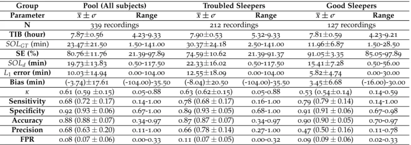
Table 6 General mean and standard deviation values over sleep statistics on
the complete pool, with emphasis on the troubled and good sleepers, as well as current classification performance measurements. For the kappa metric and conventional statistic performance measures the pooled value is given, followed by mean and standard deviation,
between brackets. 25
Table 7 General sleep statistics on different groups of troubled sleepers, as
well as some current classification performance measurements, which are presented by mean and standard deviation values. For the kappa metric the pooled value is given first, followed by the mean and
stan-dard deviation values between brackets. 28
Table 8 General sleep statistics on different groups of troubled sleepers, as
well as some current classification performance measurements, which are presented by mean and standard deviation values. For the kappa metric the pooled value is given first, followed by the mean and
stan-dard deviation values between brackets. 28
Table 9 Between brackets are the arithmetic mean and standard deviation
values obtained on κ metric, preceded by the pooled κ value. Also, means and standard deviations values obtained for SOL-detection performance measures are presented, and compared among groups of subjects, and methods of feature transformation (Norm indicates normalization and PP indicates post-processing). Significance of the difference between the results regarding L1 error and κ coefficient, obtained with different processing methods, for the same group of subjects, was calculated with a two-tailed Wilcoxon-signed rank test
[59]. ∗ p≤0.05;∗∗ p≤0.01;∗∗∗ p ≤0.001. 33
xvi List of Tables
Table 10 Mean and standard deviation values obtained for SOL-detection
per-formance over 339 recordings of mixed subjects, when varying the approach of sleep/wake classification. Significance of the difference between the results regarding L1error obtained with current classifi-cation and remaining methods calculated with a two-tailed
Wilcoxon-signed rank test. ∗ p≤0.05;∗∗ p≤0.01;∗∗∗ p≤0.001. 34
Table 11 Mean and standard deviation values obtained for SOL-detection
per-formance over 212 recordings of troubled sleepers, when varying the approach of sleep/wake classification. Significance of the difference between the results obtained with current classification and
remain-ing methods, regardremain-ing L1 error, was calculated with a two-tailed
Wilcoxon-signed rank test. ∗ p≤0.05;∗∗ p≤0.01;∗∗∗ p≤0.001. 35
Table 12 Mean and standard deviation values obtained for SOL-detection
per-formance over 127 recordings of good sleepers, when varying the approach of sleep/wake classification. Significance of the difference between the results obtained with current classification and
remain-ing methods, regardremain-ing L1 error, was calculated with a two-tailed
Wilcoxon-signed rank test. ∗ p≤0.05;∗∗ p≤0.01;∗∗∗ p≤0.001. 35
Table 13 Demographic and sleep measurement information regarding
sub-jects on the training and testing sets. 42
Table 14 List of features resultant from CFS FS on the training set, for model
M. It also contains the indication to the features which were included
to train the other models. E - Excluded. I - Included. 43
Table 15 Mean and standard deviation values obtained on the performance of
SOL-detection (L1error and estimated bias), with different classifica-tion models, on the testing set comprised of 170 recordings. Among them, are distinguished those who fit the criteria SOLGT ∈ [0, 30[ min and SOLGT ∈ [30, max]min. The significance of the differences between the results obtained with new approaches and current clas-sification, regarding L1error, within the same group of subjects, was
calculated with a two-tailed Wilcoxon-signed rank test. ∗ p ≤ 0.05;
List of Tables xvii
Table 16 Mean, standard deviation and range values regarding SOL-detection
and overall classification performance obtained with the new and current sleep/wake detection techniques, for recording of subjects with
delayed SOLGT(N=48). For some metrics, the pooled values are also
stated (before the mean and standard deviation values, which are between brackets). The significance of the difference between the re-sults obtained with new approaches andcurrent classificationmeth-ods, regarding L1 error, κ coefficient, sensitivity, specificity, accu-racy, precision and FPR, were calculated with a two-tailed
Wilcoxon-signed rank test. ∗ p ≤0.05;∗∗ p≤0.01;∗∗∗ p≤0.001. 49
Table 17 Mean, standard deviation and range values regarding SOL-detection
and overall classification performance obtained with the new and current sleep/wake detection techniques, for the complete heteroge-neous testing set, of 170 recordings. For some metrics, the pooled values are also stated (before the mean and standard deviation val-ues, which are between brackets). The significance of the difference between the results obtained with new approaches and current clas-sification methods, regarding L1error, κ coefficient, sensitivity, speci-ficity, accuracy, precision and FPR, were calculated with a two-tailed Wilcoxon-signed rank test. ∗ p≤0.05;∗∗ p≤0.01;∗∗∗ p≤0.001. 50
Table 18 Performance measures obtained for the first 31 min of recordings, on
the testing set, with models trained on the mixed (M), trouble (T) and good (G) groups of subjects, regarding the training set. The feature set for FR was altered between: CFS FS (std); union (U) and intersec-tion (I) sets. The metrics presented include pooled Cohen’s kappa for the time considered and mean and standard deviation values on SOL-detection L1 error, bias, SOLd and SOLGT. The significance of the differences between the results obtained with new approaches in comparison to current classification results (CS) calculated with a
two-tailed Wilcoxon-signed rank test. ∗ p ≤ 0.05; ∗∗ p ≤ 0.01; ∗∗∗
xviii List of Tables
Table 19 Performance measures obtained for the first 40 min of recordings, on
the testing set, with models trained on the mixed (M), trouble (T) and good (G) groups of subjects, regarding the training set. The feature set for FR was altered between: CFS (std) FS; union (U) and intersec-tion (I) sets. The metrics presented include pooled Cohen’s kappa for the time considered and mean and standard deviation values on SOL-detection L1 error, bias, SOLd and SOLGT. The significance of the differences between the results obtained with new approaches in comparison to current classification results (CS) calculated with a
two-tailed Wilcoxon-signed rank test. ∗ p ≤ 0.05; ∗∗ p ≤ 0.01; ∗∗∗
p≤0.001. 66
Table 20 Performance measures obtained for the first 50 min of recordings, on
the testing set, with models trained on the mixed (M), trouble (T) and good (G) groups of subjects, regarding the training set. The feature set for FR was altered between: CFS (std) FS; union (U) and intersec-tion (I) sets. The metrics presented include pooled Cohen’s kappa for the time considered and mean and standard deviation values on SOL-detection L1 error, bias, SOLd and SOLGT. The significance of the differences between the results obtained with new approaches in comparison to current classification results (CS) calculated with a
two-tailed Wilcoxon-signed rank test. ∗ p ≤ 0.05; ∗∗ p ≤ 0.01; ∗∗∗
p≤0.001. 67
Table 21 Performance measures obtained for the first 60 min of recordings, on
the testing set, with models trained on the mixed (M), trouble (T) and good (G) groups of subjects regarding the training set. The feature set for FR was altered between: CFS (std) FS; union (U) and intersec-tion (I) sets. The metrics presented include pooled Cohen’s kappa for the time considered and mean and standard deviation values on SOL-detection L1 error, bias, SOLd and SOLGT. The significance of the differences between the results obtained with new approaches in comparison to current classification results (CS) calculated with a
two-tailed Wilcoxon-signed rank test. ∗ p ≤ 0.05; ∗∗ p ≤ 0.01; ∗∗∗
List of Tables xix
Table 22 Performance measures obtained for the first 70 min of recordings,
on the testing set, with models trained on the mixed (M), trouble (T) and good (G) groups of subjects regarding the training set. The feature set for FR was altered between: standard (std) feature se-lection; union (U) and intersection (I) sets. The metrics presented include pooled Cohen’s kappa for the time considered and mean and standard deviation values on SOL-detection L1error, bias, SOLd
and SOLGT. The significance of the differences between the results
obtained with new approaches in comparison to current classifica-tion results (CS) calculated with a two-tailed Wilcoxon-signed rank
test. ∗ p≤0.05;∗∗ p≤0.01;∗∗∗ p≤0.001. 69
Table 23 Performance measures obtained for the first 80 min of recordings, on
the testing set, with models trained on the mixed (M), trouble (T) and good (G) groups of subjects regarding the training set. The feature set for FR was altered between: CFS (std) FS; union (U) and intersec-tion (I) sets. The metrics presented include pooled Cohen’s kappa for the time considered and mean and standard deviation values on SOL-detection L1 error, bias, SOLd and SOLGT. The significance of the differences between the results obtained with new approaches in comparison to current classification results (CS) calculated with a
two-tailed Wilcoxon-signed rank test. ∗ p ≤ 0.05; ∗∗ p ≤ 0.01; ∗∗∗
p≤0.001. 70
Table 24 Performance measures obtained for the first 90 min of recordings, on
the testing set, with models trained on the mixed (M), trouble (T) and good (G) groups of subjects regarding the training set. The feature set for FR was altered between: CFS (std) FS; union (U) and intersec-tion (I) sets. The metrics presented include pooled Cohen’s kappa for the time considered and mean and standard deviation values on SOL-detection L1 error, bias, SOLd and SOLGT. The significance of the differences between the results obtained with new approaches in comparison to current classification results (CS) calculated with a
two-tailed Wilcoxon-signed rank test. ∗ p ≤ 0.05; ∗∗ p ≤ 0.01; ∗∗∗
xx List of Tables
Table 25 Performance measures obtained for the first 100 min of recordings,
on the testing set, with models trained on the mixed (M), trouble (T) and good (G) groups of subjects regarding the training set. The feature set for FR was altered between: CFS (std) FS; union (U) and intersection (I) sets. The metrics presented include pooled Cohen’s kappa for the time considered and mean and standard deviation
values on SOL-detection L1 error, bias, SOLd and SOLGT. The
sig-nificance of the differences between the results obtained with new approaches in comparison to current classification results (CS) was
calculated with a two-tailed Wilcoxon-signed rank test. ∗ p ≤ 0.05;
∗∗ p≤0.01;∗∗∗ p≤0.001. 72
Table 26 Performance measures obtained for the first 110 min of recordings,
on the testing set, with models trained on the mixed (M), trouble (T) and good (G) groups of subjects regarding the training set. The feature set for FR was altered between: CFS (std) FS; union (U) and intersection (I) sets. The metrics presented include pooled Cohen’s kappa for the time considered and mean and standard deviation
values on SOL-detection L1 error, bias, SOLd and SOLGT. The
sig-nificance of the differences between the results obtained with new approaches in comparison to current classification results (CS)
cal-culated with a two-tailed Wilcoxon-signed rank test. ∗ p ≤ 0.05; ∗∗
p≤0.01;∗∗∗ p≤0.001. 73
Table 27 Performance measures obtained for the first 120 min of recordings,
on the testing set, with models trained on the mixed (M), trouble (T) and good (G) groups of subjects regarding the training set. The feature set for FR was altered between: CFS (std) FS; union (U) and intersection (I) sets. The metrics presented include pooled Cohen’s kappa for the time considered and mean and standard deviation
values on SOL-detection L1 error, bias, SOLd and SOLGT. The
sig-nificance of the differences between the results obtained with new approaches in comparison to current classification (CS) results
cal-culated with a two-tailed Wilcoxon-signed rank test. ∗ p ≤ 0.05; ∗∗
p≤0.01;∗∗∗ p≤0.001. 74
Table 28 List of features used with the second classifier, in the sleep/wake
clas-sification of subjects with delayed SOGT, with the new proposed
L I S T O F A B B R E V I AT I O N S
A
AASM American Academy of Sleep Medicine.
ANS Autonomic Nervous System.
B
BMI Body Mass Index.
BP Blood Pressure.
C
CFS Correlation Feature Selection.
D
DFA Detrended Fluctuation Analysis.
DS Deep Sleep. E ECG Electrocardiography. EEG Electroencephalogram. EMG Electromiography. EOG Electrooculography. F FN False Negative. FP False Positive.
FPR False Positive Rate.
FR Feature Restriction.
xxii List of Abbreviations FS Feature Selection. G GT Ground Truth. H HF High Frequency. HR Heart Rate. I
IQR Interquartile Range.
L
LD Linear Discriminant.
LF Low Frequency.
N
NREM Non-Rapid Eye Movement.
P
PPG Photoplethysmogram.
PPV Positive Predictive Value.
PSD Power Spectral Density.
PSG Polysomnography.
PSQI Pittsburg Sleep Quality Index.
R
R&K Rechtschaffen and Kales.
REM Rapid Eye Movement.
RIP Respiratory Inductance Plethysmography.
List of Abbreviations xxiii
SE Sleep Eficiency.
SO Sleep Onset.
SOL Sleep Onset Latency.
SWS Slow Wave Sleep.
T
TIB Time In Bed.
TN True Negative.
TNR True Negative Rate.
TP True Positive.
TPR True Positive Rate.
U
.
V
VLF Very Low Frequency.
W
1
I N T R O D U C T I O N
Sleep is a fundamental process that we perform with daily regularity. Even though the average human spends a third of its existence sleeping, very few people have basic knowl-edge of how sleep works. In fact, even though sleeping and dreaming have been subject of interest and inquiry since the time of the ancient Greek philosophers, it was not until the decade of 1920 that sleep was studied in terms of scientific understanding [2].
Nevertheless, from experience, and even without any scientific support, we know that a night well slept has the power to make us feel refreshed and ready to take on the world for the day ahead. On the other hand, the absence of sufficient hours of sleep can evoke terrible feelings. Based on this we can speculate on the importance of sleep: not only do we spend a big slice of our lives sleeping, but also, the quality of our sleep highly impacts the remaining time (two thirds) of our lives. This brings us to another paradoxical, however very realistic, panorama: regardless of sleep being a natural process, more than half of the adult population claims experiencing some kind of trouble or difficulty related to sleeping [3].
In the modern day, we find ourselves living as part of culture of jet lag, global travel, 24-hour cable TV, Internet addiction and shift working. Despite the advantages and infinite possibilities that our current way of living might bring, it is dramatically affecting the way we sleep. More and more people are currently suffering from sleep disorders: the World Association of Sleep Medicine (WASM) [4] has pointed out that, nowadays, up to 45% of the world population suffers from sleep-related pathologies, such as insomnia, obstructive sleep apnea, restless legs syndrome and sleep deprivation in general. These are extremely worrying numbers which situate sleep disorders among the most common illnesses of our time, even though sleep is one of the main cornerstones of good health, along with diet and exercise.
Polysomnography (PSG) is the gold standard to perform sleep detection over the length of a night of sleep [5, 6]. This is extremely important since the diagnose and treatment of sleep disorders implicate the analysis of the sleep patterns of the patient, which are accurately provided by this method. Even so, despite offering accurate physiological measurements during sleep, PSG is based on manual sleep staging, which is time-consuming, and involves high costs regarding laboratory facilities, equipment and qualified team. Automatic sleep
2 Chapter 1. introduction
stage classification, on the other hand, removes the human element from the equation and allows real-time sleep staging (useful for intervention studies) and remote monitoring (in-home sleep studies).
The electroencephalogram (EEG), as a method to measure sleep stages, has the major in-convenience of being uncomfortable for the patient and, therefore, obtrusive of sleep. Also, it requires the correct positioning of the sensors, performed by an expert.
These drawbacks have been motivating research regarding unobtrusive methods, such as sleep detection based on body movements (actigraphy) and cardiorespiratory activity [7]. Nevertheless, the performance associated with sleep staging using this technologies is still not as high as it would be desirable.
1.1 p r o b l e m d e s c r i p t i o n
One of the parameters of interest derived from sleep stages is the Sleep Onset Latency (SOL) period [8], which measures the amount of time elapsed from the instant when a per-son lies in bed with the intention to sleep until the moment when that perper-son eventually falls asleep. The SOL is a valuable indicator in the evaluation of sleep quality, sleep com-plaints and sleep disorders, such as insomnia and circadian rhythm disorders.
The problem with current unobtrusive approaches for sleep/wake classification is that they heavily rely on the idea that wake states usually coincide with periods of longer and/or more intense body movements. Actigraphy devices such as the Philips Actiwatch [9] actu-ally rely on the detection of body movements, measured with a wrist-worn accelerometer, to automatically distinguish wake from sleep. While this observation is certainly true for the majority of the night - brief periods of awakening during sleep often occur together with body movements (‘tossing and turning’ in bed) - this is not always valid at the beginning of the night, when one is trying to fall asleep. In fact, the longer it takes for a person to initiate sleep, the worse the performance of actigraphy-based sleep/wake classifiers typically is, in particular in the detection of SOL [10]. This is easily explained, given that, usually, a person will try to lie as still as possible during SOL. This is particularly common in subjects who frequently experience long SOL periods. As a result, actigraphy-based SOL estimators will very often underestimate this measure and overestimate sleep, potentially leading to an underestimation of symptoms associated with sleep disruptions or even sleep disorders. Even though introducing cardiorespiratory information has shown to improve the accuracy of sleep/wake detection [11, 7, 12], it has not completely solved the problem of the under-estimation of the SOL parameter. The main issue is that these classifiers are trained for this task with examples from the entire night and, therefore, fail to capture the particular characteristics of wake before SOL.
1.2. Objective 3
1.2 o b j e c t i v e
This work focuses on the improvement of the identification of SOL and overall sleep/wake detection based on unobtrusive cardiorespiratory signal modalities. It describes the meth-ods that proved to be most suitable for the task, as well as their application and evaluation. An increased reliability of the classification output consequently leads to the improvement of the quality of unobtrusive diagnosis/treatment equipments available for home monitor-ing and to sleep professionals. Hence, improvmonitor-ing the effectiveness rate of the treatments of sleep disorders, and, hopefully, contributing to an healthier society.
1.3 s o l u t i o n a p p r oa c h
A new classification scheme is proposed, with the intent of overcoming the limitations of the current classifier and achieving a more correct estimation of sleep/wake and SOL detection. The proposed approach includes the usage of two distinct classifiers, to be applied on subjects with delayed SOL. The first classifier is designed with the purpose of recognizing wake in the beginning of the recordings, and the other to recognize wake throughout the night. This scheme allows to compute an estimation of SOL from the scoring provided by the first classifier, and apply the second one from that moment on.
All tests performed in order investigate the topic and all results presented in this report were obtained by the development of computational routines/algorithms, using high-level
programming language and the environment MATLAB R.
1.4 o r g a n i z at i o n
The following chapter is entitled ‘Background’ and includes a theoretical description on sleep related knowledge, described in literature, which is indispensable prior to the read-ing of the remainread-ing contents of this report. Chapter 3, ‘Sleep and Wake Classification’, includes two sections. The first one, section 3.1 describes the guidelines followed to per-form sleep/wake detection, in this work. In section 3.2, ‘Current Perper-formance Assessment’, the performance of the current classifier is evaluated.
Chapter 4, ‘Experimental Study on the Performance of SOL Detection’, describes an inves-tigation on how certain aspects of the classification process influence the results on SOL detection, specifically: time of the analysis; usual quality of sleep; feature transformation methodologies and feature selection/restriction. It is organized in three sections: data set and methods; results and discussion. This is also the adopted structure for the follow-ing chapters. On chapter 5, ‘Impact of Actigraphy on the Performance of SOL Detection’, we evaluate the influence of the actigraphy feature (and correlated features) on the
per-4 Chapter 1. introduction
formance of SOL detection. Finally, on chapter 6, based on the discussions/conclusions obtained from the studies described on previously referenced chapters, a new method for sleep/wake and SOL detection is proposed and its performance is evaluated, in compari-son to currently used classifiers. Chapter 7 concludes the report with a summary of the achieved results of interest and suggestions for possible directions of feature research.
2
B A C K G R O U N D
The purpose of this chapter is to introduce the main concepts of human sleep physiology, architecture and mechanisms, which are critical to understand the approaches conducted in this research.
2.1 s l e e p h o m e o s ta s i s
In the early 1980’s, Alexander Borb´eli defined sleep homeostasis as the regulated balance between sleep and waking [13]. He presented the theory of the two-model process of sleep
regulation [13] which suggests that complex interactions between two independent physi-ological processes underlie sleep regulation. Those processes are:
• Process S, the homeostatic process (or sleep drive), which cumulatively increases during waking and decreases exponentially during sleep [13]. In other words, the longer the time we spend awake, the greater the pressure we will feel to go to sleep. By sleeping, sleep pressure is reduced and, gradually, propensity to wakefulness rises [14].
• Process C, the circadian process, is a sleep-independent mechanism that operates in cycles of approximately 24 hours, as a function of our biological clock, driven by the natural light-dark cycle of the day. The circadian process regulates distinct phys-iological rhythms, such as body temperature and hormone secretion (for example, melatonin and cortisol), which influence sleep [15]. Hence, by determining the alter-nation between cycles of high and low sleep propensity, process C is related to the regulation of sleep timing [14].
The two-process model interaction can be visualized graphically on figure 1.
As illustrated in figure 1, during a regular day of wakefulness, process S continuously builds up, inducing sleep drive. Simultaneously, process C increases its awareness effect, opposing to the latter. It is not until the alerting signal drops (usually during the evening), that sleep pressure becomes dominating enough to allow sleep to be initiated.
There are several factors that can impact the balance of our sleep-wake system [16]. For
6 Chapter 2. background
Figure 1.: The two-model process of sleep regulation: synchronized interaction between process S and C [2].
example, genetic information, stress and health conditions (such as pain and anxiety) can affect the initiation of sleep [2]. Also external factors, such as light exposure, arousal (noise), medication, caffeine and alcohol intake, among others, generally tend to increase the upper-threshold by which we fall asleep. Thus, due to the dis-synchronization between the envi-ronment and our internal biological clock, there is a fluctuation which results in a feeling of fatigue. This is why fatigue is so associated with jet lag and shift working [17].
On a cellular level, the transitioning process between the conditions of wake and sleep is controlled by brain cell interaction: some neurons are responsible for promoting wakeful-ness while others induce sleep [16]. When the alerting parts of the brain are more active they inhibit the sleep-promoting brain areas. Consequently, the state of wakefulness is present. Analogously, when the sleep-promoting areas are dominantly active, they have an inhibitory effect on the areas responsible for promoting wakefulness, resulting in sleep. This mutual inhibition can be explained by a flip-flop switch model [16], as in an electrical circuit, that either leads to the state of wakefulness or sleep, in rapid transitions. Typically, the transitions between the two states occur when the mechanism is triggered by factors related to the homeostatic sleep drive and the circadian rhythm, as explained above.
2.2 s l e e p a r c h i t e c t u r e
While sleeping, our brain exhibits distinct electrical activity, which can be measured by an Electroencephalogram (EEG) and used to characterize the process of sleep and to identify sleep stages [16].
The transition between stages occurs in a cyclic pattern which alternates between Rapid Eye Movement (REM) and Non-Rapid Eye Movement (NREM) sleep [18, 19]. The former occupies about 20 to 25% of the night, while the latter accounts for the remaining percentage. For the average healthy adult, during a typical night of sleep, approximately every 90
2.2. Sleep Architecture 7
minutes (min), the cycle repeats itself. One cycle can be discretized by order of stage
occurrence as: N1 → N2 → N3 → N2 → REM, where N1, N2 and N3 are, respectively,
the NREM stages 1, 2 and 3, which compose NREM sleep, according to the AASM [18, 19]. From 1968 to 2007, prior to establishment of the AASM rules [20], the Rechtschaffen and Kales (R&K) [21] scoring was used, and it further divided the N3 stage into stages III and IV.
Each stage will now be described, from an electroencephalographic point of view. The description is accompanied by figure 2, which reveals the typical EEG recording form for each stage.
Figure 2.: Human EEG recordings during wakefulness and sleep stages (∗sleep spindles; ∗∗slow
wave) [22]
During wakefulness, when there is a state of alertness and active mental concentration, the EEG form verified is the β-wave, which has the highest frequency and the lowest ampli-tude when compared to other sleep stages [23]. However, when a person is awake but with eyes closed, with the intention of falling asleep, as it is the case during the SOL period, the EEG records α-waves [23].
N1, often referred to as light sleep, is the first stage of sleep experienced in the cycle. It describes the transition from wakefulness (SOL period) to drowsy sleep. Hence, the EEG recordings display brain waves shifting from α-band activity toΘ-band activity (still accom-panied by brief bursts of α-activity) [23, 2]. This combination of brain activity often gives people the sensation of still being awake, when, in fact, they might already be experiencing N1 sleep. The length of this stage over an average night of sleep corresponds only to 2 to 5% of total sleep time.
8 Chapter 2. background
recordings reveal irregularities in the brain wave pattern, namely, sleep spindles (bursts of oscillatory brain activity) and K-complexes [23]. Both wave forms are illustrated, closely, in figure 3.
In comparison to the previous stage, N1, conscious awareness completely disappears [18] .
Figure 3.: EEG typical signal of the N2 stage, containing a sleep spindle, on the left, and a K-complex, on the right [16].
The succeeding stage, N3, is the deepest and most restorative stage of sleep, therefore it is known as Deep Sleep (DS) [2]. The EEG recordings reveal synchronized, low frequency
and high amplitude∆-wave activity, hence, DS is also known for the designation of Slow
Wave Sleep (SWS) [19]. During this stage, people will hardly respond to environmental stimulus and there is little (or none) muscle activity. Parasomnias, such as sleep-walking, sleep-talking and night terrors, occur during this stage [23]. It accounts for 15% to 20% of total sleep time.
Finally, the REM stage, often called paradoxical sleep [18], is characterized by a random and rapid movement of the eyes and simultaneous paralyzation of most of the body muscles [18, 19]. Despite the almost absence of movements, from an EEG point of view, REM resembles wakefulness because of the presence of desynchronized, low-amplitude and high-frequency β-waves [18, 19]. This fact makes REM sleep even more intriguing. This stage is also characterized by the ability to dream vividly; heart rate variability; irregular breathing; and Electromiography (EMG) activity [24].
The graphical representation of the sleep stages experienced by a person during the course of one night is entitled hypnogram [18]. On figure 4 there is an example of an hypnogram of an healthy adult.
As the pattern repetition proceeds, it is verified that N3 tends to diminish its length time, from each cycle to the next, while the opposite happens to REM sleep [18, 19], as observed on figure 4.
2.3. Polysomnography 9
Figure 4.: Example hypnogram of an healthy adult human over 8-hour sleep [25]. On the left side of the picture sleep stages are labeled according to the AASM rules. R stands for REM sleep. On the right side of the figure there is a description of typical predominant EEG activity associated to each stage.
2.3 p o ly s o m n o g r a p h y
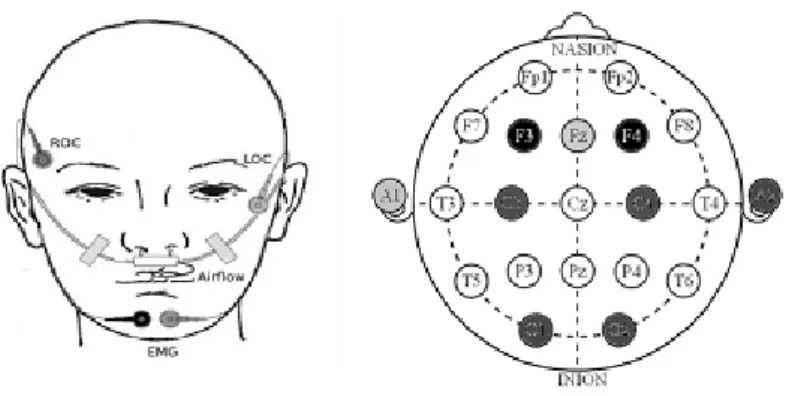
As mentioned on chapter 1, the gold standard technique to measure sleep is through PSG. It comprises monitoring of brain function, using EEG; eye movements, using Electrooculogra-phy (EOG); heart rhythm, using ElectrocardiograElectrooculogra-phy (ECG); body movements and skeletal muscle tone, using EMG; respiratory airflow, using nasal-oral thermistors and nasal pres-sure transducers; respiratory effort, using belts; and CO2 saturation, using pulse oximetry [26]. Figure 5 represents the montage of a standard PSG and figure 6 allows for a closer look into the positioning of some of the sensors, specifically those located on the face/head of the patient.
PSG recordings are performed in a sleep laboratory and the overnight sleep stages are manually scored on a 30 second epoch basis, by trained sleep experts [26, 21].
Even though the PSG provides a complete and reliable set of measurements that are of interest for sleep stage detection, the equipment is so uncomfortable, that it tends to be disruptive of sleep. Hence, a less obtrusive method is desired.
As mentioned in section 1.2 and suggested by the title of this work, the classification frame-work applied in this research makes use of only cardiorespiratory signals for the purpose of sleep stage detection, therefore being less unpleasant for the patient, and consequently less sleep disruptive of sleep.
The following section provides a description on how cardiovascular and respiratory pat-terns vary through sleep stages.
10 Chapter 2. background
Figure 5.: Drawing representing a standard PSG montage on a patient [27].
2.4 c a r d i o r e s p i r at o r y-based sleep stage classification
Cardiorespiratory activity is characterized differently on each sleep stage, hence, it is a good measure of sleep staging. The differences registered on cardiorespiratory signals during sleep are due to manifestations of the Autonomic Nervous System (ANS), which in-cludes in its structure sympathetic and parasympathetic (or vagal) activity. Between these two tones there is a balance (the sympathovagal balance) on which one activates an action while the other suppresses it [24]. For instance, a decrease on Heart Rate (HR) variability is usually linked to vagal activity, while an increase is, most likely, associated with the sym-pathetic nerves [24].
After SOL, vagal activity increases, while sympathetic activity decreases [24]. Vagal
pre-dominance during sleep is more accentuated during NREM stages. Therefore, as we
progress from wakefulness to NREM sleep there is a noticeable decrease in HR and Blood Pressure (BP), which gradually become more regular, reaching their smoothest state during N3 sleep. During periods of REM and brief awakenings, both BP and HR increase and become more variable [16].
When it comes to breathing, when we are awake, it is affected by several factors, such as: speech, emotions, exercise and posture. When we enter NREM sleep our breathing rate (BR) starts decreasing and becomes more regular, both in amplitude and frequency [30]. Also, as we progress from lighter to deeper sleep, our mean inspiratory flow decreases. On
2.4. Cardiorespiratory-based Sleep Stage Classification 11
Figure 6.: Example of a standard PSG montage sensors that are located on the head of the patient. On the panel on the left: right outer canthus and left outer canthus which, together, constitute the EOG; airflow sensors and submental EMG. At the right panel: EEG with the essential electrodes [28].
the other hand, during REM sleep, BR is irregular, with sudden changes both in amplitude and frequency, correspondent to the burst of the movement of the eyes [16].
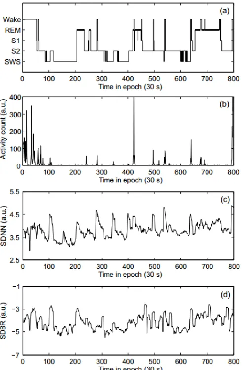
Figure 7 displays the hypnogram of an healthy subject, with correspondent activity counts and variations on BR and HR. Regarding BR and HR, there is an high correlation with the hypnogram. Regarding activity, after SOL, movements are almost absent during the course of the night, except for spontaneous peaks correlated to brief awakenings.
12 Chapter 2. background
Figure 7.: Example of sleep recordings of an healthy adult during the course of one night: (a) hypno-gram (S1 and S2 represent sleep stages N1 and N2); (b) movement counts; (c) standard de-viation of normal-to-normal heartbeat intervals (SDNN); (d) standard dede-viation of breath-ing rates (SBDR) [29].
3
S L E E P A N D WA K E C L A S S I F I C AT I O N
This chapter includes a description of the data utilized in this research and of the machine learning and statistic procedures applied. Furthermore, it addresses the status (performance-wise) of current classification methodologies available at the beginning of this work, for the task of sleep/wake detection.
3.1 d ata s e t a n d m e t h o d s
Sleep scoring is performed using supervised learning algorithms, which infer a classifica-tion output, based on examples of annotated training data. Accordingly, the data includes a set of important measurements which are assigned to a correspondent class (the label/an-notation).
3.1.1 Data Set
In this research, a data set comprising of night-recordings from 180 subjects, was used. Table 1 presents basic demographic information, such as age, gender and body mass index (BMI), and also sleep measurements acquired from the recordings, namely time spent in bed (TIB), as the amount of time elapsed from the moment of lights off until the moment of lights on; SOL time and sleep efficiency (SE), which is the proportion of sleep, during TIB, computed according to equation 1.
SE(%) = time asleep
T IB ×100; (1)
This is an adult healthy population, with a Pittsburg Sleep Quality Index (PSQI) [31] scored less than 6, that fits several criteria such as the absence of: sleep complaints; previ-ous diagnosis of sleep disorders; shift work and/or depressive symptoms.
On average, this is a population that sleeps the consensual number of hours, with reason-able SOL time, and relatively high SE [32]. Nevertheless, the standard deviation associated particularly to SOL time is high, and so is the maximum value encountered for it. This
14 Chapter 3. sleep and wake classification
Table 1.: Summary of subjects demographic information and sleep measurements
Parameter x±σ Range N 339recordings (180 subjects) Sex 98females (54.4%) Age (year) 50.10±19.68 20−95 BMI (kg/m2) 24.55±3.49 16.98-35.25 TIB (hour) 7.85±0.62 2.45-9.33 SOL (min) 23.47±21.50 1.50-141.00 SE (%) 80.76±11.76 21.39-97.89
indicates that, even though the mean values are considered ordinary and non-alerting [33], there are subjects among the population, that have experienced troubles in falling asleep, at the nights of the recordings. Considering that this an healthy population, the extended SOL times are probably due to the first night effect described in literature [34].
The information presented on table 1 refers to the grouping of recordings from 3 different data sets, namely: Boston and Eindhoven data sets, and part of the data set acquired in the SIESTA project [35].
Boston and Eindhoven data sets
The Boston and Eindhoven data sets include single-night PSG recordings and synchronized actigraphy recordings (acquired with a Philips Actiwatch [9]) of 15 healthy subjects (consid-ering the criteria mentioned above, in section 3.1.1). Nine subjects were monitored (Alice
5 PSG, Philips Respironics) in Boston, USA, during the year of 2009, at the Sleep Health
Center, while the remaining 6 were measured (Vitaport 3 PSG, TEMEC) in Eindhoven, the Netherlands, during 2010, at the High Tech Campus. Each subject provided an informed consent and the study protocol was approved by the Ethics Committee of the two sleep laboratories.
The PSG recordings are comprised of multi-channel signal modalities such as EEG chan-nels recommended by the AASM [20]; EMG; EOG; a 2-lead ECG; oxygen saturation; and thoracic respiratory effort.
Sleep stages were manually scored, on a 30-s epoch basis, by sleep experts, according to the AASM guidelines [20] as wake, REM sleep and N1-N3, for NREM sleep.
Demographic information considering subjects from the two data sets are presented on tables 2 and 3.
SIESTA regular data set
The SIESTA project [35] included sleep monitoring in seven different sleep centers, in five European locations, over a period of 3 years from 1997 to 2000. The SIESTA regular data set
3.1. Data Set and Methods 15
Table 2.: Demographics for subjects on the Boston data set.
Parameter x±σ Range N 9recordings (9 subjects) Sex 8females (88.9%) Age (year) 31.89±12.82 24−58 BMI (kg/m2) 25.31±3.81 21.00−31.20 TIB (hour) 7.09±0.48 6.56−7.69 SE (%) 91.50±3.75 86.02−97.89 SOL (min) 14.72±10.56 3.50−33.00
Table 3.: Demographics for subjects on the Eindhoven data set.
Parameter x±σ Range N 6recordings (6 subjects) Sex 2females (33.3%) Age (year) 29.67±5.92 23−36 BMI (kg/m2) 22.98±2.06 20.24−26.54 TIB (hour) 6.55±2.49 2.45−8.78 SE (%) 92.33±4.57 83.85−95.87 SOL (min) 9.83±4.83 4.00−16.50
includes only night recordings of healthy subjects, that fit the criteria mentioned in section 3.1.1. Most subjects spent two consecutive nights in the sleep laboratories. Sleep scoring was manually performed by sleep clinicians, based on all PSG channels, also on a 30-s epoch basis, according to the R&K rules [21]: wake, REM, and S1-S4 for NREM sleep. Table 4 presents demographic information regarding the subjects from the SIESTA regular data set, whose recordings were utilized in this research.
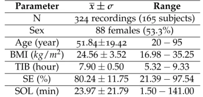
Table 4.: Demographics for subjects on the SIESTA regular data set.
Parameter x±σ Range N 324recordings (165 subjects) Sex 88females (53.3%) Age (year) 51.84±19.42 20−95 BMI (kg/m2) 24.56±3.52 16.98−35.25 TIB (hour) 7.90±0.50 5.32−9.33 SE (%) 80.24±11.75 21.39−97.54 SOL (min) 23.97±21.79 1.50−141.00
16 Chapter 3. sleep and wake classification
3.1.2 Sleep Scoring
All stages regarding sleep, either REM sleep and N1-N3 (or S1-S4) for NREM, were merged into a single class, labeled as sleep, and were labeled wake otherwise, since the purpose of this research is to distinguish sleep from wakefulness and not necessarily to distinguish between different stages of sleep. Thus, the output which results from classification, on a 30seconds epoch basis, is binary. Wake was identified as the positive class and sleep as the negative class.
In this work, SOL was recognized as the first epoch within the occurrence of three consec-utive sleep epochs (regardless of their sleep stage correspondence).
3.1.3 Framework for Sleep Stage Classification
This section presents a brief explanation of the steps involved in the automatic process of sleep classification, which was not developed during this work or by this author, but was, anyhow, utilized in this research.
Data Acquisition & Feature Extraction
As mentioned previously in section 3.1.1, the data was acquired from PSG data collection and actigraphy recordings. However, since the raw recordings are not enough to precisely characterize sleep, there is the need for a process of extracting more relevant characteristics from the recordings. Such a characteristic is named feature and such a process is referred to as feature extraction.
The feature set (collection of extracted features) used in this work comprises a total of
169features (which have all been previously described in literature and applied for sleep
staging in healthy subjects [36]), expressing information about the cardiac system; the res-piratory system; and the coupling interaction of both systems. There is an additional fea-ture which describes estimated actigraphy information from the body movement artifacts present in ECG and respiratory inductance plethysmography (RIP) [37], given that the SIESTA data set does not include actigraphy recordings.
CARDIAC FEATURES - Many based on statistics computed over R-R intervals calculated from
the QRS complexes of ECG recordings. The QRS complex is the designation of three typical waveforms of an ECG, as shown on figure 8, and the R-R interval is the time elapsed between two consecutive R waves [38].
Some features express the average HR per epoch; the nth percentile; the standard
3.1. Data Set and Methods 17
Figure 8.: Typical representation of a QRS complex of an ECG recording.
the power spectral density (PSD) analysis, regularly over three different frequency
bands: very low frequency (VLF), 0.005−0.04 Hz, low frequency (LF), 0.04−0.15
Hz, and high frequency (HF), 0.15−0.45 Hz, and from the modulus and the phase
of the pole in the HF band. Other features describe the regularity of the signal over different time scales. For instance, detrended fluctuation analysis (DFA) is used to identify longer-term correlations in the signal, and sample entropy to quantify the self-similarity of the signal over a given time period [7, 11, 12, 39, 40].
RESPIRATORY FEATURES - Based, mainly, on respiratory effort measured, for example with a
RIP belt around the thorax or around the abdomen. Several properties of respiration rate and amplitude have shown to be linked to different sleep stages [11, 41, 42]. Also, self-similarity measurements using dynamic warping have been described as useful for detecting wake states [43].
CARDIORESPIRATORY COUPLING FEATURES - Expressing the phase synchronization between
R-R intervals from ECG or beats from a photoplethysmogram (PPG), and the respiratory phase measured from RIP or from PPG during a number of breathing cycles [44, 45, 46, 47].
Feature Transformation
Following the feature extraction process, the features can be submitted to transformations in order to make them more optimized and adapted to the requirements of the classifiers. For better results, the transformation is done in two steps: normalization and post-processing.
FEATURE NORMALIZATION - Aims at reducing between-subject variability, i.e. features that
sig-nificantly vary between subjects, due to physiological or equipment-related variations. This is useful since the classifier expects a generalized model and, not having it would,
18 Chapter 3. sleep and wake classification
most likely, lead to a decrease in the accuracy of the classification. By normalizing features, they are brought to a common base line, making them more easily compara-ble between subjects.
There are different methods to normalize features which are included in the frame-work. However, they will not be described here, since exploring that is not the goal of this research.
FEATURE POST-PROCESSING - Allows the elimination of undesired components in the
fea-tures, such as long-term trends. This is extremely useful since these are components that can diminish the discriminative power of a feature over time. Again, there are several post-processing methods that can be applied, still, they will not be described in this work.
For each feature the best sets of normalizing and post-processing methods are chosen. This is a complex task which was not developed during this work and therefore will not be described in this document.
Feature Selection
Feature Selection (FS) consists in evaluating and selecting the most appropriate features for the classification task, with the goal to achieve higher classification performance. It allows faster computational time of the remaining steps to the classification process, and reduces its complexity.
The evaluation is based on attributes such as relevance, discriminatory power, redundancy and correlation between features.
Since the feature set available for this work is very wide, most likely, it will comprise redun-dant features. A feature is considered redunredun-dant if there is one or more features besides it that share its (or similar) information. By being highly correlated to other features, re-dundant features add no information to the classification. Moreover, by including more features than necessary in the training process it is likely that there will a problem of
over-fittingwhich will lower the capacity of the classifier on generalizing well to new data [48]. Therefore, redundant features should be removed from further participating in the analysis. As a result, at the end of this phase, from the complete feature set, there should be only a subset of features selected to proceed with in the classification.
In this work, the process of FS is performed by a Correlation Feature Selection (CFS) algo-rithm [49], which is based on a greedy forward search. This method starts with an empty set of features which is progressively adapted by greedily including the next best (most rel-evant) feature, according to an heuristic metric evaluation of its discriminative power and (lack of) correlation with already added features. The process stops when a desired amount of features is reached.
3.1. Data Set and Methods 19
Classification
Classification is the process of assigning each epoch to a specific class, based on the charac-teristics of that epoch, which are expressed by a feature vector. In this step, there are two desired goals: building a model that 1) provides the best possible fit and that 2) is robust against variability between subjects and performs well on unseen data.
As already referred, this work aims at investigating the binary problem of the identification of each epoch as sleep or wake. For this classification problem a Bayesian Linear Discrimi-nant (LD) classifier [50] was used. Previous sleep research has proved that the LD classifier is the most adequate for the task of sleep/wake detection [7]. The basic idea behind the LD algorithm, introduced by Fisher, is to find a linear discriminant that yields a maximum separation between two classes [50].
Classification requires a training phase, so that the classifier can be designed and modeled to available example data, and a testing phase, to estimate the error rate of the trained classifier. Training and testing samples must be different and statistically independent, in order to get reliable predictions in future classification [51].
Over time, more than one way of combining training and testing samples for error estimation has been proposed:
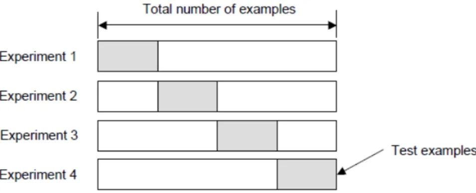
HOLD-OUT [51] - this method suggests that the available data should be split into two
disjoint subsets, as exemplified on figure 9, for a single train-test experiment. One group is used for the task of training including FS while the other is held for the task of testing.
Figure 9.: Exemplified distributions of examples as training and testing subsets.
One limitation of this method is that it is not appropriate if the data set available is small. Generally, in those conditions, the testing set is valuable for training and, by having set it aside, the performance of the prediction will be compromised, leading to biased results. Notwithstanding, in the case of not so small data sets, data will still be wasted.
Another drawback of this method is that, since the results are so dependent on the choice of the training/testing set of samples, they will be misleading in the event of an unfortunate division. For instance, it might be too easy/difficult to classify certain examples of data in the testing set, leading, again, to biased results.
20 Chapter 3. sleep and wake classification
CROSS-VALIDATION [52] - an alternative method that overcomes the difficulties associated to
the hold-out method, at the cost of more computations. It still consists in performing the training and testing on separate subsets of data, but the process is repeated several times.
One type of cross-validation is the K-fold cross-validation, according to which the data is partitioned in K bins of approximately equal size and the model is trained and validated K times in a loop. Figure 10 exemplifies a splitting of the data and training/testing according to this model.
Figure 10.: Sample K-fold cross-validation with K=4.
The idea is that, on each experiment, K−1 folds are used for training and the
re-maining one for testing. FS occurs on the data that is not left out, during each cross-validation loop.
The main advantage of this method is that, at the end of the process, all examples have been used for both training and testing. The overall performance is computed based on the average performance achieved in each fold. Hence, the result is less sensitive to the partitioning of the data set and more accurate.
3.1.4 Performance Assessment
On the next chapters of this report, several performance metrics will be referenced. Some will be related to SOL-detection performance while others to the overall epoch-by-epoch sleep scoring. To facilitate and avoid repetitions, all measures are listed and briefly ex-plained below.
3.1. Data Set and Methods 21
L1ERROR (MIN) - Taxicab or Manhattan distance, which represents the length between two vectors p and q in an n-dimensional real vector space:
L1(p, q) = N
∑
i=1
|pi−qi| (2)
In this work, this metric is applied to the vectors of the measurements of the
de-tected SOL moment (min) from classification, SOLd, for each recording, and the
computed SOL time (min) from ground truth (GT) labels, SOLGT, for the same
recordings.
BIAS (MIN) - Difference between SOLd and SOLGT, computed, for each recording, ac-cording to equation 3:
Bias= SOLd−SOLGT (3)
For a given group of recordings regarding L1error or bias values, the arithmetic mean (or just mean), x, and standard deviation, σ, are computed according to equations 4 and 5, respectively [53]. The arithmetic mean is a measure of central tendency which is used in this work with the intent of summarizing statistics on a certain metric. The standard deviation is computed with the goal of addressing how spread out the data is. x= 1 N N
∑
i=1 xi (4) σ= v u u t1 N N∑
i=1 (xi−x)2 (5)Where xi is either a value regarding L1error or bias, for a given recording i, in a group of recordings, of size N.
In order to visualize the comparison of SOL-detection performance between different approaches of classification, the Bland-Altman plot [54] will be used. It aims at pro-viding an answer on whether two methods are comparable enough to the point where one could replace the other. This kind of plot is more suitable for method comparison than the obvious plot of one method against the other, because with the latter, the
![Figure 1 .: The two-model process of sleep regulation: synchronized interaction between process S and C [ 2 ].](https://thumb-eu.123doks.com/thumbv2/123dok_br/17554356.816887/30.892.144.666.157.383/figure-model-process-sleep-regulation-synchronized-interaction-process.webp)
![Figure 2 .: Human EEG recordings during wakefulness and sleep stages ( ∗ sleep spindles; ∗∗ slow wave) [ 22 ]](https://thumb-eu.123doks.com/thumbv2/123dok_br/17554356.816887/31.892.248.695.400.708/figure-human-recordings-during-wakefulness-sleep-stages-spindles.webp)
![Figure 4 .: Example hypnogram of an healthy adult human over 8 -hour sleep [ 25 ]. On the left side of the picture sleep stages are labeled according to the AASM rules](https://thumb-eu.123doks.com/thumbv2/123dok_br/17554356.816887/33.892.162.795.153.371/figure-example-hypnogram-healthy-picture-stages-labeled-according.webp)
![Figure 5 .: Drawing representing a standard PSG montage on a patient [ 27 ].](https://thumb-eu.123doks.com/thumbv2/123dok_br/17554356.816887/34.892.151.665.155.548/figure-drawing-representing-standard-psg-montage-patient.webp)
![Figure 11 .: Sample Bland-Altman plot for method comparison [ 54 ].](https://thumb-eu.123doks.com/thumbv2/123dok_br/17554356.816887/46.892.224.591.325.663/figure-sample-bland-altman-plot-method-comparison.webp)