Stress Tests on European Banks:
Determinants of Banking Failure
Pedro Miguel dos Santos Silva
Dissertation submitted as partial requirement for the conferral of
Master in Finance
Supervisor:
Professor José Joaquim Dias Curto, Associate Professor
ISCTE Business School, Quantitative Methods Department
Co-supervisor:
Professor Paulo Viegas de Carvalho, Invited Assistant Professor
ISCTE Business School, Finance Department
Abstract
Banks are very unique entities essential to the actual society, since generally every single individual needs one at least once in his life. Besides being a rare event, banking failures consequences are quite dramatic do society. A bank failure is different from a non-financial corporation failure, since the impact to society is bigger. With a bank failure, arises the possibility of a contagion effects and the possibility of destruction of clients’ trust in the whole sector. Banks are also the main financing source of both families and companies.
Stress tests started to be executed by large financial institutions to trading books, in order to assess their potential losses under extremely adverse market conditions. The emergence of several crises, namely the recent sovereign debt crisis, changed stress tests from a small-scale exercise to a bigger-scale exercise and gave them an important role in policy.
This dissertation identifies the determinants of stress tests results in Europe. To achieve this goal, a Pooled Logit model was estimated with stress tests results as dependent variable and using as explanatory variables bank specific variables, like financial ratios, and macroeconomic variables of the bank’s home country.
The results showed that both financial and macroeconomic variables influence the probability of stress tests failure. However, with the overcoming of the economic crises that haunted Europe in the last decade, and with the growth of banking regulation/supervision, the probability of a European bank failing stress tests and consequently having problems that could cause bankruptcy, has decreased.
Key Words: Bank Distress; Risk; Stress Tests; Supervision JEL Codes: C23; G21
Resumo
Os bancos são entidades únicas e essenciais para a sociedade atual. Apesar de ser um evento raro, a falência de bancos tem um enorme impacto na sociedade. É este impacto que distingue a falência de um banco e a falência de uma empresa não financeira, uma vez que o impacto para a sociedade é maior no primeiro caso. Com a falência de um banco, surge a possibilidade de efeitos de contágio e de destruição da confiança dos clientes no setor, sendo os bancos a principal fonte de financiamento de particulares e empresas.
Os testes de stress começaram a ser desenvolvidos por grandes instituições financeiras, que os aplicavam a trading books. Com o surgir de várias crises, nomeadamente com a recente crise das dívidas soberanas, os testes de stress passaram de um exercício em pequena escala para um exercício de grande escala, começando ainda a ter um importante papel na política.
Para identificar os determinantes que explicam os resultados dos testes de stress à banca europeia, foi estimado um modelo Pooled Logit utilizando os resultados dos testes como variável binária dependente e como variáveis explicativas variáveis específicas dos bancos, como rácios financeiros, e variáveis macroeconómicas do país de cada banco.
Os resultados mostram que quer os rácios financeiros, quer as variáveis macroeconómicas, influenciam a probabilidade de falha nos testes de stresss. No entanto, com o ultrapassar das crises económicas e com o crescimento da supervisão bancária, a probabilidade de um banco falhar nos testes, e de poder vir a falir, diminuiu.
Palavras-Chave: Falência; Risco; Supervisão; Testes de Stress Códigos JEL: C23; G2
Acknowledgements
1To my supervisors, who help me and support me until the end of this journey.
To Banco de Portugal, especially to my co-workers and coordinators, whose personalities challenged me to research and learn more.
To André Dias, André Fernandes, Fábio Santos, Francisco Felisberto, José Soares, Rafael Figueira and Ricardo Correia for their precious help.
To my family, especially to my parents for their decision to not invest in financial markets but in their son and for their eternal support and patience.
To my girlfriend, who never gave up on me and whose love, support and affection kept me in the right way.
To my friends, a particular group of individuals whose fantastic support and unbelievable personalities made me stronger.
1 The opinions and arguments contained in this report are the sole responsibility and not of ISCTE-IUL or of the
I
Table of Contens
1. Introduction ... 3
2. Literature Review ... 5
2.1 A brief stress tests history ... 5
2.2 Classification ... 6
2.3 Methodologies ... 7
2.4 Limitations ... 8
2.5 European Banking Authority Stress Tests ... 9
2.6 Models ... 12 3. Database ... 19 4. Methodology ... 22 4.1 Model Type ... 22 4.2 Model Variables ... 24 4.3 Initial Model ... 35 5. Estimation Results ... 36 5.1 Data Description ... 36
5.2 Final Model Development ... 37
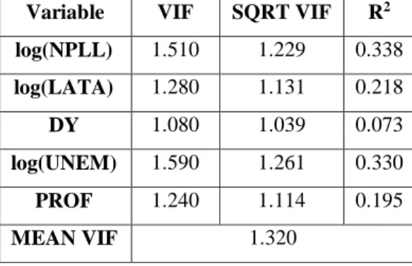
5.3 Final Model Quality ... 46
5.4 Coefficients Analysis ... 50
5.5 Marginal Effects Analysis ... 51
6. Projection ... 53
7. Conclusion ... 55
8. References ... 58
9. APPENDIX ... 63
A. Stress tests classification ... 63
B. Significant macroeconomic drivers ... 64
C. Significant banking drivers ... 65
II
E. Unemployment rate of the bank’s country ... 67
F. Banks stressed ... 68
G. Intermediate Pooled Models ... 77
H. Intermediate Random Effects Models ... 81
Table of Figures
Figure 1 Banks Funding - Source: Beau, 2014 ... 11Figure 2 Model Variables - Source: Betz et al. 2013 ... 17
Figure 3 Percentage of banks countries to total banks analyzed each year - Source: EBA ... 21
Figure 4 Real GDP growth rate in volume (%) - Source: Eurostat ... 28
Figure 5 2016 Non-performing loans across countries (%) - Source: WorldBank ... 29
Figure 6 Amount outstanding of debt securities issued by banks in EU [28] - Source: ECB ... 31
Figure 7 Portuguese and German 10 years yield curve - Source: Bloomberg ... 33
Figure 8 Area under the ROC curve ... 49
Figure 9 Stress Testing of Financial Systems: Overview of Issues, Methodologies, and FSAP Experiences - Source: Blaschke et al. ... 63
Figure 10 Inflation rate - Source: Eurostat ... 66
Figure 11 Unemployment rate by country - Source: Eurostat ... 67
Table of Tables
Table 1 Bank percentiles for 2014 ... 34Table 2 Bank percentiles for 2016 ... 34
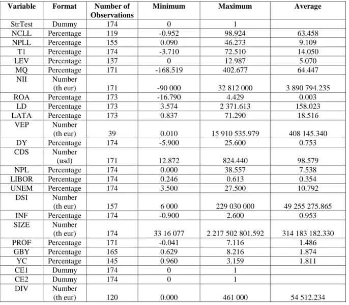
Table 3 Descriptive Statistics ... 36
Table 4 Pooled Final Models ... 38
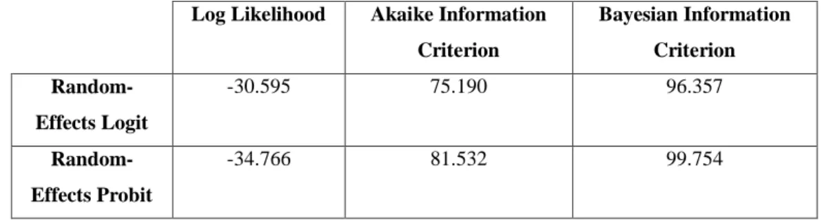
Table 5 Random Effects Final Models ... 39
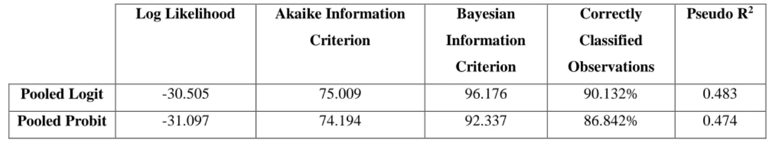
Table 6 Comparative statistics between Pooled Logit and Pooled Probit Models ... 40
Table 7 Comparative statistics between Pooled Logit and Pooled Probit Models ... 41
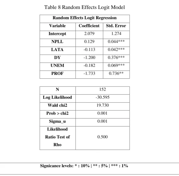
Table 8 Random Effects Logit Model ... 42
Table 9 Comparative statistics between Pooled and Random Effects Model ... 44
Table 10 Final Model with logarithmic forms ... 45
III
Table 12 Variance Inflation Factors (VIF) of Final Model ... 47
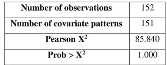
Table 13 Person chi-square goodness-of-fit Test ... 49
Table 14 Hosmer-Lemeshow goodness-of-fit Test ... 49
Table 15 Marginal Effects ... 51
Table 16 Banks stressed in 2018 ... 53
Table 17 Significant macroeconomic drivers - Source: Kapinos et al. ... 64
Table 18 Significant banking drivers - Source: Kapinos et al. ... 65
Table 19 Re-estimated initial models - Pooled ... 77
Table 20 Table 19 re-estimated models without DSI, GBY and CDS ... 78
Table 21 Table 20 re-estimated models without DSI, GBY and CDS ... 79
Table 22 Re-estimated initial models – Random Effects ... 81
Table 23 Table 21 re-estimated Models ... 82
“Science is the great antidote to the poison of enthusiasm and superstition.” Adam Smith (1776:418)
3
1. Introduction
The theme of this thesis is stress tests, a theme barely developed in Portugal and an important theme regarding the financial sector of the economy. Alexander (2008:378) refers that “If estimating VaR is like playing a pianola then stress testing is like performing on a
concert grand.”, so it can be demonstrated that stress tests are a large scale and a spotlight event
in which the performance of regulators will be analyzed.
Banks are crucial entities in the current society, and a banking failure2 is a striking event. Banking failures are different from non-financial corporations’ failures, since a unique bank failure can put at risk the clients trust and trigger the collapse of the entire banking system. This is the reason why banks are more supervised and controlled by authorities (Kick and Koetter, 2007).
Stress tests at a regulatory level started to be developed in the 1990’s, when financial institutions encouraged risk managers to go beyond the standard risk metrics and to imagine circumstances that could create extreme losses (Alexander, 2008). They jumped into the spotlight with the 2007’s tremendous financial crisis. The crisis peaked with the Lehman Brothers bankruptcy in the United States and continued in Europe with the sovereign debt crisis (Kouretas and Vlamis, 2010). Regulatory entities decided subsequently that is of extremely importance to supervise more clearly and efficiently the banking system, to prevent this type of events, because during crisis the potential losses that stress tests predicted were less than the losses that really occurred (Dent et al., 2016).
In the field of stress tests, the focus are the European banks, mainly the biggest and most important of the region. In Europe, stress tests are conducted by the European Bank Authority (EBA), but they were originally directed by the Committee of European Banking Supervisors (CEBS) in 2009, immediately after the beginning of the crisis in an attempt to prevent more losses and to control the financial system.
Since 2009, Europe suffered lots of transformations, namely in the economic conditions of the region. So, one point to analyze is the evolution of the methodology applied by EBA. We
4
also want to compare this methodology with other alternatives applied in different countries or regions and by different authorities.
The main objective of this thesis is to discovery the determinants that influence the result of stress testing. Using an econometric model, we intend to answer the question why banks fail stress tests and then discuss the consequences of the failure to the financial sector.
The possible relevant variables are specific bank variables, like financial ratios, and macroeconomic variables and were mainly based in the CAMELS3 Rating System.
However, stress tests are not a concept widely known by the population, even for people specialized in finance, so it is also important to explain the concept, focusing in their origin, purpose and importance.
Having all this in mind, the research questions are presented below:
Why there is a specific methodology applied to stress tests in Europe? And why there is not a different one?
What determines the banks performance in stress testing and why? (key question) What are the consequences for the banks that fail this kind of tests?
At the end, attempting to show that reality can be explained by this dissertation and to check the robustness of our model, we will test its predictive accuracy by projecting 2018 stress tests results.
5
2. Literature Review
The starting point of this essay is the concept of stress tests. In Finance, stress testing is a method used to access the risk associated to a portfolio. However to calculate the risk associated to a portfolio there are risk measures, like value-at-risk (VaR).
The key usefulness of stress tests comes from the usage that financial regulators give to them. Supervision authorities use stress tests to evaluate the fragilities of the financial system. The main difference between stress test applied to portfolios and the ones applied by the regulators to the entire financial system are the objectives. In stress tests regulators want to identify the main vulnerabilities of the financial system and the overall risks, while stress tests applied to portfolios want to examine if there is an efficient allocation of capital according to risks (Blaschke et al, 2001).
For Oura and Schumacher (2012) stress testing is defined as a technique that measures vulnerability of a portfolio based on hypothetical scenarios relatively to institutions or to an entire financial system. According to Jorion (2006), the same concept is used to identify and manage extreme unusual situations that can cause huge losses. Also based on Jorion (2006) statements, the main differences between the two referred risk measures (value-at-risk and stress testing) are the conditions under which the losses occur. Value-at-risk calculates the potential losses under normal market conditions, while stress testing quantifies it for extreme market conditions, like a crisis.
Focusing more in the regulatory framework, Dent et al. (2016) state that stress testing is mainly used to assess the resilience of a bank, when it faces rare, but plausible, shocks that can cause huge losses. Stress tests can also be used to access if the bank management is performing a good job, testing the future of the bank under the natural evolution of the economy.
2.1 A brief stress tests history
Stress tests started to be used in the 1980’s, as a tool of primordial risk management used to specific large risks (Kapinos et al., 2015). In the early 1990’s, financial institutions, like banks, started to apply stress tests focused in the trading books (Blaschke et al., 2001; McGee and Khaykin, 2014), being this measure formalized in 1996 with an amendment to the international regulatory capital regime for market risk.
After the emergence of stress tests conducted by banks, policymakers started to use them to evaluate the resilience of the financial sector of the economy. This kind of tests became a crucial component of the Financial Sector Assessment Program (FSAP) created in 1999 due to the Asian Financial Crisis (Independent Evaluation Office of International Monetary Fund,
6
2004) and were performed by all countries that belong to the program. With this program, banks have taken more initiative, starting to develop and produce their own stress tests (Dent et al., 2016). Until the financial crisis of 2007, stress tests in Europe were only limited to banks following the Internal Rating-Based Approach for Capital Requirements for Credit Risk (Basel Committee on Banking Supervision - Bank for International Settlements, 2001). In 2007, the collapse of Lehman Brothers triggered the so-called US subprime crisis. According to Kouretas and Vlamis (2010), this crisis led indirectly to the origin of the sovereign debt crisis in the Eurozone.
With the recession, it was proved that deficiencies in risk measurement exist, since stress tests showed a better scenario than it actually occurred, being the real losses bigger than the estimated ones (Basel Committee on Banking Supervision - Bank for International Settlements, 2009). The financial crisis implied the largest financial reform since the 30’s Great Depression, and changed the way stress tests were performed with regulation purpose, transforming stress tests from an isolated exercise with small-scale to a more general and large-scaled exercise (Dent et al., 2016).
The first example of this new regulation stress tests was the US Supervisory Capital Assessment Program (SCAP), conducted by the Federal Reserve in early 2009. In Europe, the first tests of this kind were conducted in late 2009 under the direction of the Committee of European Banking Supervisors (CEBS). After this and since the beginning of 2011, the European Banking Authority (EBA) started to conduct these tests.
To conclude, we can say that before the crisis stress tests had none or little direct impact in policy, but this situation changed after the 2007’s crisis (Dent et al., 2016).
2.2 Classification
In 2001, Blaschke et al.4 define several criteria to classify stress tests at the portfolio level, namely the type of the risk model, analyses, shock or scenario.
Regarding the type of risk model, stress tests can be applied in order to check the vulnerabilities of the institutions against credit risk, operational risk or market risk. Credit risk is defined as the risk that a counter-party will default its obligations (Blaschke et al., 2001). Operational risk is the risk resulting from losses related with failed internal processes, people and from external events (Basel Committee on Banking Supervision - Bank for International
7
Settlements, 2001). Market risk is the risk associated with losses coming from changes in the market prices (Blaschke et al., 2001).
Focusing on the type of analyses, three classifications arise. The first one is the sensitivity analyses (single-factor) stress tests, which consist in a sensitivity test that only varies a single factor without considering the relations of this factor with other factors (International Actuarial Association, 2013). It is commonly used to assess potential hedging strategies. The second stress test analysis is the multi-dimensional/scenario that, according to Jorion (2006) is process that based on a plausible event varies several risk factors. This analysis reflects several individual risk factors and the interaction between them, and it is generally used to assess particular situations. The third and final type of analysis is the extreme value or loss, used to quantify the losses of an extreme event (Embrechts et al., 1999).
Stress tests can also be classified depending on the type of shock, and so, in relation to this subject they can be allocated in three categories: underlying volatilities, underlying correlations or individual market variables. The first two categories, make stress tests scenarios designed to include changes in relationships between market variables, while the last one only makes stress tests scenarios designed to only take into consideration individual market variables, like prices.
Finally, stress tests can weight different type of scenarios, namely historical, hypothetical and Monte Carlo simulation scenarios. According to Alexander (2008) historical scenarios are based on events that occurred in the past and whose data is applicable to the present, in order to obtain the potential losses if that event occurs again. For hypothetical scenarios, the same author states that this type of tests does not need historical precedent, since they are scenarios created with the only purpose of stress testing. The last type of scenario is Monte Carlo simulation, which according to Allen (2013) consists in identifying plausibility with some type of probability measure and applying it to the different possible events, making regulators to consider only the losses caused by a few events that have at least a certain probability of happening.
2.3 Methodologies
According to Dent et al. (2016) stress tests carried out by regulators that affected simultaneously several financial institutions are called concurrent stress tests. This kind of tests can be performed through several approaches, being balance sheet, market price-based models
8
and macro financial models the main ones (Jobst et al., 2013). Jobst et al. (2013) also explain in more detail the three main approaches.
The balance sheet approach is the oldest, the simplest, the most widely used and it has the advantage of producing direct results in terms of regulatory variables.
The market price-based models approach was developed based on risk management techniques and defines “systematic risk measures” based on dependencies between different risk factors. Unlike the balance sheet approach, market price-based models take into consideration the possibility of institutions fail simultaneously (joint default risk) and the sensitivity of stress test results to the historical volatility of risk factors when they defined the capital adequacy under stressful conditions. The main disadvantages of this approach are the fact that it does not produce direct results in terms of regulatory variables, needing additional steps and the fact that this approach is likely to include valuation methods and so tends to be less tractable.
Lastly, macro financial models are used to examine systemic risks that arise from the relations between the macroeconomic and financial environments. This approach can be implemented simultaneously with one of the two previous models.
The topic of this essay is related with concurrent stress tests of European banks, which as it was previously referred are conducted by EBA. The approach used by EBA is a balance sheet, more specific a static one, meaning that the bank balance sheets do not change through the forecast horizon. EBA run a joined-up adverse macro scenario with a three-year horizon, which is developed by the European Central Bank and European Systemic Risk Board (ESRB) with the purpose of capturing the systemic risks that represent the biggest threats to the stability of the European financial sector (Dent et al., 2016).
2.4 Limitations
Stress testing is an important and revolutionary technique, however as other techniques it is not perfect, and so it has limitations. According to the Committee on the Global Financial System - Bank for International Settlement (2000) the main limitation of stress tests is the fact that they depend a lot from the regulator choices in for example, what risk factors to stress or how to combine factors stressed.
9
Regulators choice have also an important role in analyzing the results of stress testing and identifying the implications that those results have in the bank, making the strategy of the bank to manage risk dependent of their interpretation.
For the Committee on the Global Financial System (2000), another important limitation is the fact that the main stress tests processes can determine the possible loss but cannot associate a probability to this loss.
Based on Dent et al. (2016) the limitations of stress tests are derived from the fact that stress tests are only a tool and consequently cannot be a substitute for the entire robust capital framework, they can only complement it. Another limitation that these authors refer is related with the robustness of stress testing, since stress tests are more or less robust depending on the robustness of the data and methodologies used.
2.5 European Banking Authority Stress Tests
EBA is one of the three entities that are part of European System of Financial Supervision (ESFS), being the other two entities the European Securities and Markets Authorities (ESMA) and the European Insurance and Occupational Pensions Authority (EIOPA). The date of foundation of EBA is 1st of January of 2011.
The two main functions of EBA are the promotion of equal supervisory practices, to achieve a harmonized prudential system and to evaluate the main risks and vulnerabilities of the European banking sector. It is in the framework of this last function that stress tests were performed by EBA, in close cooperation with the European Systemic Risk Board (ESRB).
Stress tests are considered one of the most important tools to assess the resistance of European financial institutions to adverse shocks, contributing also to assess the systematic risk of European financial system.
Since 2011, year of its foundation, EBA concluded three series of stress tests. The first one was performed in 2011, the second in 2014 and the last one in 2016. This type of tests is performed in a bank-by-bank basis and the sampled banks should have at least have a minimum of 30 thousand million euros in assets or the total sample of banks from a specific country should cover at least 50% of the country banking sector.
The type of adverse shocks that European financial institutions hypothetically face are adverse macro-economic scenarios, like crisis. The impact of such shock is measured in terms
10
of the Common Equity Tier l Ratio5 (CET1). A bank passes or fails stress tests depending on the value of Tier 1 capital. The choice of CET1 comes mainly from the decision of EBA to select a simple measure and a measure that can be issued directly by the bank.
EBA defines capital hurdle rates for both baseline (obtained from economic forecasts regarding the main macroeconomic variables) and adverse scenarios. If the Transitional Common Equity Tier 1 Ratio6 of the bank is below the defined threshold under the baseline or adverse scenario, the bank fail stress tests. Otherwise, if the bank has a Transitional Common Equity Tier 1 Ratio over the defined threshold, he passes the stress tests with success, being resilient against the adverse scenario shock and meaning that management is performing a good job under normal conditions (baseline).
EBA stress tests assume a static balance sheet, a zero-growth assumption. This assumption should be applied to both assets and liabilities. The Profit and Losses, the revenues and the costs, should also admit the zero-growth assumption. Another assumption is that banks maintain the same business mix and model throughout the time horizon.
The main risks that EBA stress tests intend to assess are: Credit risk
Market risk Sovereign risk Securitization Cost of funding
Credit risk is the risk that a borrower may not pay a loan, with banks losing the principal of the loan or the interest associated.
Market risk is the risk associated to the possibility that a bank, as investor, suffers losses due to factors that affected negatively the performance of the financial markets. This type of risk is also called systematic.
5 Ratio of the bank’s common equity tier 1 (primarily consists of ordinary shares, retained earnings and certain
reserves) to its total risk-weighted assets.
6 CET1 ratio with the application of transitional arrangements, such as phase-in of deductions and grandfathering
11
Sovereign risk is related with possibility that a foreign central bank changes its regulations, leading to a reduction or completely nullifying the value of its foreign exchange contracts. In this type of risk is also included the default in debt repayments by a foreign nation. Securitization is a complex process that uses financial engineering to transform an illiquid asset or group of illiquid assets into securities. The risks associated to this process increase when the complexity of the instruments increase, making harder the analysis of the future security performance. With instruments complexity increases the lack of transparency, making even worst the forecast of the security performance (Sabarwal, 2009).
Cost of funds is the interest rate paid by banks to obtain money to finance their activities. The spread between the cost of funds and the
interest rate charged is one of the most important sources of profit of the financial institutions. The risk in this type of process comes when the cost of funding increases. If the cost of funding increases, the bank has three options. First, charge a bigger rate on loans, finding new costumers and making profit in these new loans. Second, keep the same rate, finding
new costumers and losing money in this new loans. Third, charge a bigger rate on loans, but did not find new costumers, losing also money (Beau et al., 2014).
Figure 1, show us that must exist a balance between the assets held by the banks and the cost of the funds. If this balance is not achieved problems may rise and consequently banks can fall in distress.
For the 2016 stress tests results, EBA changed its approach and do not classify stress tests results as failures or successes, deciding only to communicate the banks risks to the country supervisors and doing efforts in the sense of keeping the capital in the banking system and repairing the unbalanced balance sheets. For the 2018 stress tests series, currently in course, EBA uses a similar approach.
12
2.6 Models
2.6.1 CAMELS Rating System
The CAMELS Rating System, officially Uniform Financial Institutions Rating System (UFIRS), was implemented in 1979 in the US banking institutions. This rating system analyses the banking sector through the balance sheets and profit and loss statements of the banks. Until 1997, the system abbreviation was CAMEL, reflecting the five assessment areas: capital, asset quality, management, earnings and liquidity ratios. In 1997, a sixth area was added (sensitivity to market risk), and the system abbreviation stated to be CAMELS.
For each assessment area there is a rating, leading to an overall rating of the bank’s financial condition. The ratings are from 1 to 5; the bigger the rating, the higher the supervisory concern.
The ratios used to evaluate the financial situation of the banks are the following: Capital Adequacy Ratio
It is the ratio of Tier I (common and preferred stocks, convertible bonds and bank’s minority rights in Subsidiary companies) and Tier II (bank supplementary capital) capital to risk-weighted assets, being the Tier I at least 50% of the risk-risk-weighted assets value.
The higher the ratio, the better is the bank’s capital adequacy, meaning that the bank can benefit from self-financing and be more profitable than other banks.
Asset Quality Ratio
It is the ratio of non-performing loans over 90 days less provisions (capital held by the bank to compensate delays in loans payments) to total loans.
A lower ratio value, means that the quality of the assets is higher. Management Quality Ratio
It is the ratio of total operating expenses to sales.
13
Earnings Ratio
The earnings and profitability of the bank can be assessed by two ratios: Return on Equity (ROE) and Return on Assets (ROA).
ROE is the ratio of net profits to own capital and ROA is the ratio of net profits to total assets.
The higher the value of each one of the ratio, the more efficient is the bank. Liquidity Ratio
To assess the liquidity of the bank there are two ratios: L1 and L2.
L1 is the ratio of total deposits to total loans, while L2 is the ratio of circulating assets (cash in hand, investment portfolios, etc.) to total assets.
The higher the ratios, the higher the bank’s liquidity. Sensitivity to Market Risk Ratio
It is the ratio of total securities to total assets. This ratio relates a bank’s total securities portfolio with its assets and gives us the percentage change of its portfolio based on changes on the issuers of the securities or on the interest rates, for example. A smaller ratio value indicates that the bank portfolios are less susceptible to market risk.
2.6.2 Kick and Koetter (2007)
In 2007, Kick and Koetter developed a model to estimate the probabilities of financial distress in German banks.
The data was collected from the records of Bundesbank about distress events in German universal banks for the period of 1997 to 2004. The non-distress bank observations were included in one group. Then the distress events were categorized in four categories, according to their severity. In the first category were inserted the events that cause a reduction of annual operational profits of more than 25% or events that cause losses amounting to 25% of liable capital or events that may put at risk the existence of the bank as a going concern. In the second category, were introduced events that capture actions taken by the Federal Financial Supervisory Authority (BaFin) representing official warnings or disagreement. The third category includes events that caused the bank to receive support in the form of capital from his head association or events that cause bank operations to be limited by the BaFin. Finally, in the
14
last category were included the events that caused a forced closure of the bank by the BaFin or events that caused takeovers of the bank by other banks, denominated restructured mergers.
The model developed by Kick and Koetter was a logit model: 𝑃(𝑌𝑖> 1) = 𝑔(𝛽𝑗𝑋𝑖) 𝑒𝑥𝑝(𝛼𝑗+𝛽𝑗𝑋𝑖)
1+𝑒𝑥𝑝(𝛼𝑗+𝛽𝑗𝑋𝑖), 𝑓𝑜𝑟 𝑗 = 1,2, 𝑀 − 1 (1) M number of event classes
𝑋𝑖 vector of explanatory variables 𝑎; 𝛽 parameters to estimate
The vector of explanatory variables includes financial variables, macroeconomic variables of the bank’s country and a dummy variable that equals one if the bank had a distress in the past.
The main deductions were that loan quality, cost efficiency and capitalization7 have big status to explain distress, but cost efficiency and capitalization are only explanations for events of small distress8. Another main conclusion is that banks with past situations of distress will have a higher probability of facing a new distress in the future. It was also concluded that it is difficult to prevent a bank failure, when a certain level of distress has been achieved.
2.6.3 Čihak and Poghosyan (2011)
In 2011, Čihak and Poghosyan, developed a model to find the determinants of bank distress in Europe. The data was compiled based on two different sources, the Bureau Van Dijk’s BankScope database and the NewsPlus database.
BankScope provided financial data for 5 708 banks in the EU-25 countries for the period of 1996 to 2007, and The NewsPlus database provided information to discover failing banks. Due to this last search, it was discovered 79 distress events in 54 banks.
In order to assess the impact of financial indicators in the probability of a bank distress, several versions of a Logistic (Logit) probability model were used, following Shumway (2001).
7 An increase in the capitalization ratio reduces the effect of category I and II of banks distress events
15
The principal model can be represented in the form of a log odd’s ratio: 𝑙𝑜𝑔 𝑃𝑖𝑗
1−𝑃𝑖𝑗
= 𝛽0 + ∑𝐾𝑘=1𝛽𝑘𝑋𝑘,𝑖𝑗𝑡−1 (2)
𝑃𝑖𝑗 probability that bank i located in country j will experience distress in period t X vector of K explanatory variables
𝑙𝑜𝑔 𝑃𝑖𝑗 1−𝑃𝑖𝑗
log odd’s ratio, measuring the probability of bank distress relative to the probability of no distress
Two different approaches can be applied to this model. The simplest one assumes independence of errors across individual banks, countries, and time, and estimates a logit. The second approach, is also to estimate a logit model, but including random effects9. The explanatory variables used in the models are financial indicators, namely capitalization, asset quality, managerial skills, earnings, and liquidity, macroeconomic variables of the bank’s country residence, a measure of market concentration and stock market indicators.
The main conclusions are that capitalization has an important role on bank distress, but asset quality and earnings have even a bigger impact. Also, contingency effects have an important role in banks distress, with results showing that banks that perform their activity in a more concentrated market have more probability to suffer a distress. Lastly, another variable that increases the probability of a bank distress is the higher share of wholesale funding.
2.6.4 Apergis and Payne (2013)
Apergis and Payne (2013) create a Probit model to identify the impact of credit risk and macroeconomic factors in the prediction of European bank failures. In order to control for heteroscedasticity problems, they decide to apply robust estimation, which consist in a robust “sandwich” estimator for the asymptotic covariance matrix of the quasi-maximum likelihood.
The model consists in the following:
𝑦𝑖 = 𝑥𝑖𝛽 + 𝛼𝑖 + 𝜀𝑖 (3)
εi = 1
y binary variable with 1.0 for failure to pass the stress test, and 0.0 otherwise α individual country-specific effect
9 Random effects assumes that the variation across the banks is random and uncorrelated with the independent
16
β vector of parameters, it is estimated by using the cluster corrected covariance matrix method of maximum likelihood and Newton’s method
i bank i
The study includes data from 90 banks across 21 countries, for the years of 2010 and 2011. The type of variables were both macroeconomic variables, related with the country of the bank, and banking variables.
The main conclusions were that both type of variables are significant when we are talking about bank failures. Contributing to a higher probability of bank failure are greater ratios of non-performing loans to total loans and non-current loans to loans, lower capital adequacy ratios based on the Tier I capital, a higher leverage ratio, lower management quality, and a lower net interest income ratio. The same pressure to the risk of failure derives from lower returns on assets, a higher loans to deposits ratio, a lower ratio for liquid assets to total assets, greater variance of a bank’s equity price, lower GDP growth, higher CDS, spreads, bigger overall banking non-performing loans ratio in the country of the bank and a higher LIBOR.
Another conclusion is that supervisory authorities have access to signals that can indicate a possible bank failure. Also, bank risk managers can detect those signals when looking into the intrinsic variables.
2.6.5 Betz et al (2013)
Betz et al. (2013) developed a model to predict distress in European banks using macroeconomic variables and bank specific variables. Behind their selection of variables is the CAMEL rating system, created in 1979 by the US regulators (section 2.6.1). The sample used consisted of quarterly data for 546 banks with at least EUR 1bn in total assets, and, since 2000Q1 until 2013Q2, corresponding to a total of 28 832 observations.
Since bank distress is a rare event when we are talking about European banks, a proxy was necessary and so, Betz et al. (2013) define as distress events bankruptcies, liquidations, defaults, forced mergers and state intervention.
The model used was a pooled logit model with bank distress as a dependent and dummy variable and the following variables tested as explanatory:
17
Figure 2 Model Variables - Source: Betz et al. 2013
The main results are that both bank specific variables and macroeconomic variables for economic imbalance and banking sector vulnerabilities are relevant for banking distress prediction. The inclusion of both type of variables improves the model performance.
2.6.6 Kapinos et al. (2015)
Kapinos et al. (2015) use a top-down approach to create a method to stress testing banks. The method assesses the impact of several macroeconomics shocks on banks capitalization, and is based on a variable selection that identifies the main macroeconomic drivers that influence specific bank variables.
The approach also allows to identify the financial statement variables that contribute to bank heterogeneity, due to the response to macroeconomic shocks. The sample is composed by 156 US banks with assets at least of $10 billion for at least one quarter during the period from 2000Q1 to 2013Q3. For these banks, the data used was public quarterly data.
The model was estimated using two different dependent variables, pre-provision net revenue (PPNR) and net charge-offs (NCO) on all loans and leases, being PPNR = (interest income + noninterest income) - (interest expense + noninterest expense).
In order to recognize the relevant macroeconomic drivers, they use a least absolute shrinkage and selection operator (LASSO) approach (Tibshirani, 1996). This approach was used first to find the significant macroeconomic drivers for each of the banking variables of
18
interest, and then, in a second step, using the set of variables discovered by LASSO as significant, an index of macroeconomic conditions was generated (Appendix B).
The same method was applied concerning the income statement and balance sheet variables, to find the relevant variables (Appendix C).
For each of the dependent variables, several specifications of the following model were estimated: 𝑌𝑖𝑡 = 𝛼𝑖+ 𝛽𝑗𝑌𝑖𝑡−1+ ∑ 𝛾𝑗,𝑝𝑓𝑡 𝑝 + 𝑣𝑖𝑡 𝑃 𝑝=1 (4) P = 1,3 number of different situations tested
j associated with the coefficients β and γ reflects three alternative empirical strategies
β and γ coefficients i bank i
t period
α specific effects
The first empirical strategy, standard-fixed effects, is an approach where only the vertical intercepts differ from one bank to another, 𝛽(𝑗) = 𝛽 and 𝛾(𝑗) = 𝛾. The second is the time series, which is an approach where the all coefficients are estimated for individual banks, 𝛽(𝑗) = 𝛽𝑖 and 𝛾(𝑗) = 𝛾𝑖, for i = 1,…,n. The third is the estimation of fixed-effects models which permits coefficients to vary for groups of banks based on their income statement and balance sheet characteristics, 𝛽(𝑗) = 𝛽𝑔 and 𝛾(𝑗) = 𝛾𝑔, for g = 1,…, G.
The main results point to an improvement in banking capitalization10 in the recent years, however this type of shocks still have a significant impact in the deterioration of banks capital positions. Other conclusion was that macroeconomic variables can be drivers of banking variables.
19
3. Database
The main purpose of this dissertation is to find the key determinants of stress testing, namely which factors or variables can define if a bank fails or passes in the tests.
The model has a dummy depended variable that assumes the value 1 if the bank fails stress tests and 0 otherwise. In relation to the explanatory variables, we use bank specific variables, like financial ratios, macroeconomic variables and two variables to assess contagion effects.
According to Wooldridge (2012), data used to estimate models can be of three types, namely cross-section, time series and panel data. Cross-section data is collected at the same time for several different individuals or institutions. Time series data is collected for the same individual or institution, but at different points in time. Finally, panel data is the combination of both, consisting in a time series for each cross-sectional data presented in the sample. In stress tests, there are several banks analyzed in each series, which is the cross-sectional part of the data, but since in this dissertation we want to analyze more than one stress tests series (several years), we also have a time series component as part of the data, classifying our data as panel data.
Also based on Wooldridge (2012), panel data can be balanced or unbalanced. In this case our data is unbalanced, since one bank can be analyzed in the 2011 stress tests series, but there is no obligation that the same bank needs to be analyzed in another stress tests series. The banks selected to the stress tests are only defined by the regulators criterions, which can change the sampled banks for each stress tests series.
The focus is in the data of the banks submitted to the stress tests of 2011, 2014 and 2016 in Europe. To collect this type of information, we used Bloomberg, European Central Bank (ECB), WorldBank and Eurostat for the macroeconomic variables and EBA, Yahoo Finance
20
and Orbis for the specific bank variables. Being Orbis, a Bureau Van Dijk database, the main source of data.
Since EBA assumes a static balance sheet for the banks, the information of the variables were collected for the year before the stress tests series. For example for the 2016 stress tests series the information collected for the variables relates to 2015.
To identify banks that failed the stress tests and obtain their information, we used the specialized financial media and the results published by EBA.
Next, we describe briefly the stress tests of 2011, 2014 and 2016. In 2011, EBA conducted stress tests over 90 banks, and 8 of them failed the stress tests, since their CET1 were smaller than 5% under the baseline or under the adverse scenario. The 8 (9.00% of the total banks analyzed) banks that failed were: Oesterreichische Volksbank AG (Austria), EFG Eurobank and Agricultural Bank (Greece), and Caja de Ahorros del Mediterráneo, Catalunya Caixa, Banco Pastor, Unnim and Caja 3 (Spain). Due to the lack of data and to the high number of banks that no longer exist, this year was excluded from the database, except the information regarding the banks who failed, which will influence the dummy variable CE211.
In 2014, 123 banks were assessed by stress tests, from which 25 failed (20.00% of the total banks analyzed), since their CET1 under baseline scenario were smaller than 8.00% or their CET1 under adverse scenario were inferior to 5.50%. These 25 banks were: Oesterreichische Volksbank AG (Austria), Dexia and Axa (Belgium), Hellenic Bank and Bank of Cyprus (Cyprus), C.H.R. (France), Münchener Hypothekenbank eG (Germany), Eurobank, National bank of Greece and Piraeus Bank (Greece), Permanent tsb plc. (Ireland), Banca Carige S.P.A., Banca Piccolo Credito Valtellinese, Banca Popolare Dell'Emilia Romagna, Banca Popolare Di Milano, Banca Popolare di Sondrio, Banca Popolare di Vicenza, Veneto Banca S.C.P.A., Banca Monte dei Paschi di Siena S.p.A. and Banco Popolare (Italy), Coöperatieve Centrale Raiffeisen-Boerenleenbank B.A. (Netherlands), Banco Comercial Português Portugal), Nova Ljubljanska banka and Nova Kreditna Banka Maribor (Slovenia) and Liberbank (Spain). From the previous banks, 16 were below the defined thresholds for both
11 Dummy variable used to access if a bank fail in a previous stress tests series affects the behavior/result in another
21
baseline and adverse scenario, 8 were only below the threshold defined for the adverse scenario and only one was below the baseline scenario and above the adverse scenario.
In 2016, the stress tests were performed to about 51 banks. One limitation regarding the stress tests results in this year is that it wasn’t defined a threshold to analyze if a bank fails or passes the stress tests. However, assuming the 2014 stress tests thresholds (transitional CET1 below 8.00% under the baseline scenario and 5.50% under the adverse scenario) the only bank that would fail the stress tests in 2016 is Banca Monte dei Paschi di Siena S.p.A., which presented a CET1 under adverse scenario of -2.23%.
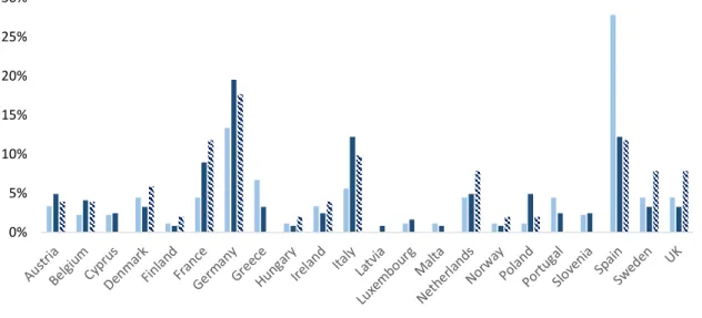
Based on figure 3, we can conclude that Spain, Germany and Italy were the countries that had a higher percentage of banks analyzed in each stress tests series.
Figure 3 Percentage of banks countries to total banks analyzed each year - Source: EBA
0% 5% 10% 15% 20% 25% 30% 2011 2014 2016
22
4. Methodology
4.1 Model Type
The main objective of this dissertation is to find the main determinants of stress tests results for banking institutions.
To achieve this objective, the econometric model should present as dependent variable the stress tests results (pass or fail). Since this type of variable has clearly restricted values, this model is considered a limited dependent variable model (Wooldrigde, 2012).
𝑃(𝑦 = 1|𝑥) = 𝐺(𝛽0 + 𝛽1𝑥1+ ⋯ + 𝛽𝑘𝑥𝑘) = 𝐺(𝛽0+ 𝑥𝛽) (5) G function taking on values strictly between zero and one
In the category of limited dependent variable model, logit and probit are the most commonly used. The main difference between both is related with the type of G function used. In the probit model the function used is the standard normal cumulative distribution function:
𝐺(𝑧) = 𝛷(𝑧) = ∫−∞𝑧 𝛷(𝑣)𝑑𝑣 (6) In the logit model the function used is the logistic cumulative distribution function:
𝐺(𝑧) = exp(𝑧) /[1 + exp(𝑧)] = ⋀(𝑧) (7) The dataset that serves this dissertation is considered panel data. The panel data
regressions, can have cross section effects, time effects or both.
For this type of data, three subtype of models can be estimated, namely Pooled Ordinary Least Squares, Random-Effects Model and Fixed-Effects Model.
Regarding the first one, a Pooled Ordinary Least Squares is simply an Ordinary Least Squares technique to estimate panel data, in which individual-specific and time effects are totally ignored.
𝑦𝑖𝑡 = 𝑥𝑖𝑡𝛽 + 𝑣𝑖𝑡′ (8) i bank i
t period where
23
𝑣𝑖𝑡 = 𝑐𝑖+ 𝑢𝑖𝑡
This regression is only consistent if the error term is not correlated with the regressors. 𝑐𝑜𝑣(𝑥𝑖𝑡, 𝑣𝑖𝑡) = 0
x regressors v error
However, even if the covariance between the regressors and the error is zero, composite error are serially correlated.
So, to estimate sing this kind of model, it is necessary a robust variance matrix estimator and robust test statistics.
About Random Effects Model, the situation is different. In this kind of model, individual-specific effects are taken into account and are considered a random variable, which is not correlated with explanatory variables. The model also assumes that the cross-section part of the data was chosen as a random sample.
𝑦𝑖𝑡 = 𝑥𝑖𝑡𝛽 + 𝑐𝑖𝑡+ 𝑢𝑖𝑡 (9) where 𝐸(𝑢𝑖𝑡| 𝑥𝑖1, 𝑥𝑖2, … , 𝑥𝑖𝑇, 𝑐𝑖) = 0 𝐸(𝑐𝑖𝑡| 𝑥𝑖1, 𝑥𝑖2, … , 𝑥𝑖𝑇) = 0 𝑣𝑎𝑟(𝑢𝑖𝑡| 𝑥𝑖, 𝑐𝑖 ) = 𝑣𝑎𝑟(𝑢𝑖𝑡) = 𝜎𝑢′2 𝑣𝑎𝑟(𝑐𝑖| 𝑥𝑖) == 𝜎𝑐′2 𝑐𝑜𝑣(𝑢𝑖𝑡, 𝑢𝑖𝑠| 𝑥𝑖, 𝑐𝑖) = 0
Finally, the Fixed Effects Model. In this type of model, individual-specific effects is a random variable that is allowed to be correlated with the explanatory variables. The model also assumes that the cross-section part of the data was chosen as a random sample.
𝑦𝑖𝑡 = 𝑥𝑖𝑡𝛽 + 𝑐𝑖𝑡+ 𝑢𝑖𝑡 (10) where
24
𝑣𝑎𝑟(𝑢𝑖𝑡| 𝑥𝑖, 𝑐𝑖 ) = 𝑣𝑎𝑟(𝑢𝑖𝑡) = 𝜎𝑢′2 𝑐𝑜𝑣(𝑢𝑖𝑡, 𝑢𝑖𝑠| 𝑥𝑖, 𝑐𝑖) = 0
The idea for estimate the coefficients is to transform the equations in order to eliminate the unobserved effect 𝑐𝑖.
The Fixed Effects transformation is obtained by first averaging the 10 equation:
𝑦̅𝑖𝑡 = 𝑥̅𝑖𝑡𝛽 + 𝑐𝑖𝑡+ 𝑢̅𝑖𝑡 (11) 𝑦𝑖𝑡 − 𝑦̅𝑖𝑡 = (𝑥𝑖𝑡− 𝑥̅𝑖𝑡)𝛽 + 𝑐𝑖𝑡+ 𝑢𝑖𝑡 − 𝑢̅𝑖𝑡 (12) The independent variables or explanatory variables used are bank specific variables, like ratios, macroeconomic variables regarding the bank’s country and two variables measuring the possible contagion effects. Most of these variables are based on the CAMEL rating system and in the presented in the literature review.
4.2 Model Variables
4.2.1 Stress Tests (StrTest)
The dependent variable of the model is the stress tests results, pass or fail. It is a dummy variable that equals 1 if bank i fails the stress test in period t and 0 if bank i does not fail the stress test in period t.
4.2.2 Non-Current Loans to Total Loans ratio (NCLL)
Non-Current Loans to Total Loans ratio is defined as the ratio of loans that will not mature in the next 12 months and the total loans.
According to Spong and Sullivan (1999), non-current loans to total loans ratio provides a clear measure to analyze the loan quality. A high ratio indicates a worse credit risk management, and so a bigger probability of a bank distress. So, it is expected that 𝛽̂2 presents a positive sign, since non-current loans to total loans ratio is positively correlated with the dependent variable.
4.2.3 Non-Performing Loans to Total Loans ratio (NPLL)
Non-performing loans to total loans ratio is the ratio of the non-performing loans to total loans, being non-performing loans defined as a loan in default or quasi in default. According to Čihak and Poghosyan (2011), the data on non-performing loans is not available for a use amount
25
of banks, so can be used a proxy by the ratio of loan loss provisions to total loans, being loan loss provision the amount of money that banks have to cover losses from bad banks.
Bigger non-performing loans to total loans ratio leads to bigger vulnerability and increases the probability of bank failure, a conclusion stated by Apergis and Payne (2013). It is also one variable used in the CAMELS Rating System (section 2.6.1). So, it is expected that 𝛽̂3 presents a positive sign, since non-performing loans to total loans ratio is positively correlated with the dependent variable.
4.2.4 Tier 1 Capital ratio (T1)
Tier 1 capital is the ratio of banks core capital to its total risk-weighted assets, is the mandatory capital that banks are required to hold in addition to other minimum capital requirements. According to Apergis and Payne (2013), increases in Tier 1 capital reduce the probability of bank failure in the stress tests, because a higher Tier 1 means that the is more capital to absorb possible losses. So, it is expected that 𝛽̂4 presents a negative sign, since Tier 1 capital ratio is negatively correlated with the dependent variable.
When we are trying to collect data for T1 ratio, some of the banks (around 13% of the observations) do not have available this variable. However Common Equity Tier 1 (CET1), a component of this ratio is available for the entire set of observations.
CET1 plus Additional Tier 1 (AT1) are equal to Tier 1, being CET1 compose mostly by common stocks. Besides losing the AT1 effect (mostly composed by preferable shares and other high convertible instruments, like securities) a bigger CET1 also indicates that the bank has more capital to absorb possible losses, so it is expected that 𝛽̂4 still presents a negative sign.
4.2.5 Leverage ratio (LEV)
T1 Leverage ratio is the ratio of Tier 1 Capital (CET1) to total assets, it is also the inverse of the capitalization ratio. According to Čihak and Poghosyan (2011), leverage is one of the most discussed topics as an indicator of bank security. Čihak and Poghosyan also state that a higher leverage ratio makes the bank more sensitive to shocks. So, it is expected that 𝛽̂5 presents a positive sign, since leverage ratio is positively correlated with the dependent variable.
26
4.2.6 Management Quality ratio (MQ)
Management Quality ratio, is the aptitude of the bank managers to minimize expenses, it is the ratio of operating expenses to total revenues. According to Čihak and Poghosyan (2011) and Apergis and Payne (2013), a higher management quality ratio denotes a greater aptitude of managers to reduce expenses, decreasing the probability of bank failure. It is also one variable used in the CAMELS Rating System (section 2.6.1). So, it is expected that 𝛽̂6 presents a negative sign, since management quality ratio is negatively correlated with the dependent variable.
4.2.7 Net Interest Income (NII)
Net Interest Income is the difference between revenues generated by interest-bearing assets and the cost of servicing (interest-burdened) liabilities, it is the lending margin charged.
Since a loan is priced in accordance to its risk, a more risky loan will have a bigger price. A bigger lending margin charge is due to riskier loans, which present a high probability of default, consequently increase the probability of a bank failure (Apergis and Payne, 2013). However, according to Schmieder et al. (2011), net interest income is the most important source of income for banks. So, assuming that the income effect is greater than the risk effect associated to a higher net interest income, it is expected that 𝛽̂7 presents a negative sign, since net interest income is negatively correlated with the dependent variable.
4.2.8 Return on Assets (ROA)
Return on assets is measured as the ratio of net profit to average total assets and it measures the profitability of a bank. According to Apergis and Payne (2013), a higher return on assets denotes a higher prospection of banks growth, reducing the probability of a bank failure. It is also one variable used in the CAMELS Rating System (section 2.6.1). So, it is expected that 𝛽̂8 presents a negative sign, since return on assets is negatively correlated with the dependent variable.
4.2.9 Loans to Deposits ratio (LD)
Loans to deposits ratio is the ratio between the total loans and the total deposits of the bank. Deposits, as debt issuance and shareholders’ equity are main sources of funds of a bank, being deposits the most stable source of funding. Bigger loans to deposits ratio, means that banks prioritize as source of funds other sources than deposits, increasing the credit risk
27
(Apergis and Payne, 2013). It is also one variable used in the CAMELS Rating System (section 2.6.1). So, it is expected that 𝛽̂9 presents a positive sign, since loans to deposits ratio is positively correlated with the dependent variable.
4.2.10 Liquid Assets to Total Assets ratio (LATA)
Liquid Assets to Total Assets ratio is the ratio between the total of liquid assets held by a bank and the total of its assets. Liquid assets are assets that can be changed for money quickly. The faster and more easily they can be converted into cash, the more liquid they are. They can be measured as the difference between equity and deposits plus loans, according to a classical microeconomic theory (Alger and Alger, 1999).
According to Alger and Alger (1999), the interbank market is one important source of funding, however it is very expose to credit risk, which can collapse the market. When a bank seeks for more liquidity in the interbank market, it will find difficulties if the respective probability of insolvency is high. Banks invest in liquid assets to prevent a collapse in the interbank market, and in order to cover large deposits withdrawals as a consequence of that collapse.
According to Apergis and Payne (2013), a bigger liquidity ratio makes the bank more resilient to liquidity crises, reducing the probability of a bank failure. So, it is expected that 𝛽̂10 presents a negative sign, since liquidity assets to total assets ratio is negatively correlated with the dependent variable.
4.2.11 Variance of Bank’s Equity price (VEP)
12For measuring the market risk, it is used the variance of bank’s equity price during a certain year. According to Ötker-Robe and Podpiera (2010), equity volatility measures the uncertainty of risk associated to an investment in the bank’s equity. Apergis and Payne (2013) based in this analysis, conclude that a bigger equity volatility is associated to a bigger market risk, which increases the perspective of a bank failure.
Not all the banks presented listed shares, moreover most of them have unlisted shares. For the banks without unlisted shares, there is no way of estimate the variance of equity price based in the shares quotes, so VEP will not have value for these banks. In practice, this variable also works as a dummy, which is 1 for the listed banks and 0 for the unlisted banks. So, it is
28
expected that 𝛽̂11 presents a positive sign, since variance of bank’s equity price is positively correlated with the dependent variable.
To cover events that do not change the market cap of the bank, but that affect the bank’s stock price, like a stock split, the variance is calculated based on the adjusted closing price.
4.2.12 GDP Growth of the Bank’s country (DY)
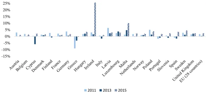
GDP growth is one of the key indicators of economic health. If the economy is growing, there is less risk of a bank failure (Apergis and Payne, 2013). In Europe the countries that presented the worse GDP growth were the peripheral countries, with the exception of Ireland (table 4).
In 2013, Mayes and Stremmel find that GDP growth has good predictive power and a negative effect when predicting banks distress. So, it is expected that 𝛽̂12 presents a negative sign, since GDP growth is negatively correlated with the dependent variable.
Figure 4 Real GDP growth rate in volume (%) - Source: Eurostat
4.2.13 Credit Default Swap Spread of the Bank’s country (CDS)
Credit default swap is the most liquid of credit derivatives currently traded, being a derivative that transfers the credit risk from one investor (protection buyer), who is exposed to the risk, to another investor (protection seller), who is willing to accept that risk. The protection seller charges a fee (CDS spread) to the protection buyer, in exchange of his commitment to
-15% -10% -5% 0% 5% 10% 15% 20% 25% 30% 2011 2013 2015
29
compensate the protection buyer if a default event occurs before maturity of the contract (Blanco et al., 2005).
When the risk of default increases, the CDS spread also increases, leading the protection seller to ask for a higher fee to assume the risk. According to Apergis and Payne (2013), a higher CDS spread implies a greater underlying risk, increasing the probability of a bank failure. So, it is expected that 𝛽̂13 presents a positive sign, since credit default swaps spreads are positively correlated with the dependent variable.
4.2.14 Non-Performing Loan ratio of the Bank’s country (NPL)
The same variable as the one stated at point 4.2.3, but applied at the bank’s country level. So it is expected that 𝛽̂14 presents a positive sign, since non-performing loans to total loans ratio is positively correlated with the dependent variable.
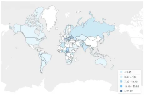
From the countries analyzed in this dissertation the one that stands out is Italy with NPL loans in the range of 14.40% to 20.92% (Figure 5).
Figure 5 2016 Non-performing loans across countries (%) - Source: WorldBank
4.2.15 Libor– OIS
13Spread (LIBOR)
Libor-OIS spread is the difference between Libor interest rate and the overnight indexed swap rate. The Libor interest rate is the London interbank offer rate, which is the rate that bank
13 Overnight Index Swap, which are an interest rate swap involving the overnight rate being exchanged for a
30
specify to lend to other banks. The OIS rate, designated overnight index swap, is the rate on a derivative contract on the overnight rate (Thornton, 2009).
The Libor-OIS spread started to have an important role in measuring the health of banks with the 2007 crisis, since until then the spread was close to zero. This spread reflects the risk to lend to other banks, so the higher the spread, the higher is the risk of lending, and consequently the bigger the probability of a bank failure (Apergis and Payne, 2013). So, it is expected that 𝛽̂15 presents a positive sign, since Libor-OIS spread is positively correlated with the dependent variable.
4.2.16 Unemployment rate of the Bank’s country (UNEM) (appendix D)
The unemployment rate is the percentage of the total labor force that is unemployed but actively seeking employment and willing to work. According to Makri et al. (2013) the unemployment rate is one of the determinants of the non-performing loans, because households’ unemployed present less income and the probability of defaulting their loan payments increases, and consequently increasing the probability of a bank failure.
Also based on Klein (2013) from the International Monetary Fund, the level of non-performing loans tends to increase when the unemployment rate increases, at least in the Central and Eastern and Southeastern European countries.
The bigger the unemployment rate, the bigger the percentage of defaulting costumers, so it is expected that 𝛽̂16 presents a positive sign, since the unemployment rate is positively correlated with the dependent variable.
4.2.17 Debt Securities issued (DSI)
Banks can finance themselves through deposits, shareholders’ equity or debt issuance. An issue of debt securities increases the total debt, making the responsibilities of the bank increase. A debt securities issuance is a source of founding that as to be repaid, and sometimes include regular payments, for example like bond coupons. If, the bank present already a fragile situation this source of financing will increase this fragility of the bank, making more probable a bank failure. So it is expected that 𝛽̂17 presents a positive sign, since debt securities issued are positively correlated with the dependent variable.
31
Figure 6 Amount outstanding of debt securities issued by banks in EU [28] - Source: ECB
Analyzing the amount outstanding of short-term and long-term debt securities issued by banks of European Union [28], we can conclude that the amount of long-term debt securities is much superior to the amount outstanding of short-term debt securities (Figure 6), in mean the amount outstanding of the short-term debt securities correspond to 13.26% of the amount outstanding of the long-term debt securities. It means that banks preferred to finance themselves with long-term securities. In this model the total debt securities issued corresponds to the sum of short-term and long-term debt securities issued.
4.2.18 Inflation rate of the Bank’s country (INF) (appendix E)
The inflation rate measures how fast prices of goods and services rise over time and it is a major concept in macroeconomics. According to Demirguc-Kunt and Huizinga (2000) banks generally profit in environments of inflation, so the probability of a bank failure decreases. It is expected that 𝛽̂18 presents a negative sign, since the inflation rate is negatively correlated with the dependent variable.
4.2.19 Banks Size (SIZE)
One way of measuring a bank size is to analyze the value of its assets. The bigger the assets owned, the greater is the size (Laeven et al., 2014).
According to Laeven et al. (2014), usually large size banks present a higher systematic and individual risk than smaller banks. The risk of a large bank increases when it has insufficient capital or when it presents unsustainable funding. Also, large banks, being a complex corporation structure have more probabilities to fail. From the social welfare perspective banks are too large to operate.
1 000.00 2 000.00 3 000.00 4 000.00 5 000.00 6 000.00 7 000.00 8 000.00 2017 2016 2015 2014 2013 2012 2011 2010 2009 2008 2007 2006 2005 2004 2003 2002 AO of Short-term deb securities AO of Long-term deb securities
Th o u san d mi lli o n e u ro s
32
There are banks considered too big to fail, which assets growth at a higher rate than their country’s economy, even in crisis. The number of these banks decreases, but the remaining ones became even bigger. However, recent results showed that these banks are not immune to failure. Deutsche Bank, one of the biggest 2000’s banks, is facing huge problems, mainly due their poor management performance, demonstrating that even the too big to fail banks have risk of collapse. So, it is expected that 𝛽̂19 presents a positive sign, since banks size is positively correlated with the dependent variable.
4.2.20 Banks profitability (PROF)
Net interest margin can be calculated as the difference between the investment returns and the investment expenses, divided by the average earning assets. It is considered a better measure of profitability of banks than for example return on assets, since studies show that the net interest margin of banks start to decline before a crisis, while the return on assets stayed more stable in those situations (Saksonova, 2014).
A bigger bank profitability measured by the net interest margin decreases the probability of a bank failure, and so, it is expected that 𝛽̂20 presents a negative sign.
4.2.21 Government Bond Yields (GBY)
Government bonds are bonds issued by a government. The government bond yield is the rate that governments pay to borrow money for different lengths of time. The higher the yield, the greater the possibility of government default, since investors demand a higher rate to compensate the higher risk.
A bigger probability of a government default denotes problems in the economy, namely a recession, increasing the probability of a bank failure. So it is expected that 𝛽̂21 presents a positive sign, since government bond yields are positively correlated with the dependent variable.