Stationary Black Holes: Uniqueness and Beyond
Piotr T. Chru´sciel
University of Vienna email: [email protected] http://homepage.univie.ac.at/piotr.chrusciel
Jo˜ao Lopes Costa
Instituto Universit´ario de Lisboa (ISCTE-IUL), Lisboa, Portugal Centro de An´alise Matem´atica, Geometria e Sistemas Din^amicos, Instituto Superior T´ecnico, Universidade T´ecnica de Lisboa, Portugal
email: [email protected]
Markus Heusler
ITP, University of Zurich, CH-8057 Zurich (at the time of writing original 1998 version)
email: [email protected]
Accepted on 29 March 2012 Published on 29 May 2012
Abstract
The spectrum of known black-hole solutions to the stationary Einstein equations has been steadily increasing, sometimes in unexpected ways. In particular, it has turned out that not all black-hole–equilibrium configurations are characterized by their mass, angular momentum and global charges. Moreover, the high degree of symmetry displayed by vacuum and electro-vacuum black-hole spacetimes ceases to exist in self-gravitating non-linear field theories. This text aims to review some developments in the subject and to discuss them in light of the uniqueness theorem for the Einstein–Maxwell system.
This review is licensed under a Creative Commons
Attribution-Non-Commercial-NoDerivs 3.0 Germany License. http://creativecommons.org/licenses/by-nc-nd/3.0/de/
Institute for Gravitational Physics, Am M¨uhlenberg 1, 14476 Potsdam, Germany. ISSN 1433-8351. This review is licensed under a Creative Commons Attribution-Non-Commercial-NoDerivs 3.0 Germany License: http://creativecommons.org/licenses/by-nc-nd/3.0/de/. Figures that have been previously published elsewhere may not be reproduced without consent of the original copyright holders.
Because a Living Reviews article can evolve over time, we recommend to cite the article as follows:
Piotr T. Chru´sciel, Jo˜ao Lopes Costa and Markus Heusler, “Stationary Black Holes: Uniqueness and Beyond”,
Living Rev. Relativity, 15, (2012), 7. [Online Article]: cited [<date>], http://www.livingreviews.org/lrr-2012-7
Fast-track revision A fast-track revision provides the author with the opportunity to add short notices of current research results, trends and developments, or important publications to the article. A fast-track revision is refereed by the responsible subject editor. If an article has undergone a fast-track revision, a summary of changes will be listed here.
Major update A major update will include substantial changes and additions and is subject to full external refereeing. It is published with a new publication number.
For detailed documentation of an article’s evolution, please refer to the history document of the article’s online version at http://www.livingreviews.org/lrr-2012-7.
29 May 2012: Major update of the original version by Markus Heusler from 1998. Piotr T. Chru´sciel and Jo˜ao Lopes Costa succeeded to this review’s authorship. Significantly restructured and updated all sections; changes are too numerous to be usefully described here. The number of references increased from 186 to 329.
1.1 General remarks . . . 7
1.2 Organization . . . 8
2 Definitions 9 2.1 Asymptotic flatness . . . 9
2.2 Kaluza–Klein asymptotic flatness . . . 9
2.3 Stationary metrics . . . 9
2.4 Domains of outer communications, event horizons . . . 10
2.5 Killing horizons . . . 11
2.5.1 Bifurcate Killing horizons . . . 11
2.5.2 Killing prehorizons . . . 12
2.5.3 Surface gravity: degenerate, non-degenerate and mean-non-degenerate horizons 12 2.6 I+-regularity . . . 15
3 Towards a classification of stationary electrovacuum black hole spacetimes 16 3.1 Static solutions . . . 16
3.2 Stationary-axisymmetric solutions . . . 17
3.2.1 Topology . . . 17
3.2.2 Candidate metrics . . . 17
3.2.3 The reduction . . . 18
3.2.4 The Robinson–Mazur proof . . . 19
3.2.5 The Bunting–Weinstein harmonic-map argument . . . 19
3.2.6 The Varzugin–Neugebauer–Meinel argument . . . 19
3.2.7 The axisymmetric uniqueness theorem . . . 19
3.3 The no-hair theorem . . . 20
3.3.1 The rigidity theorem . . . 20
3.3.2 The uniqueness theorem . . . 20
3.3.3 A uniqueness theorem for near-Kerrian smooth vacuum stationary spacetimes 22 3.4 Summary of open problems . . . 22
3.4.1 Degenerate horizons . . . 22
3.4.2 Rigidity without analyticity . . . 24
3.4.3 Many components? . . . 24
4 Classification of stationary toroidal Kaluza–Klein black holes 26 4.1 Black holes in higher dimensions . . . 26
4.2 Stationary toroidal Kaluza–Klein black holes . . . 27
4.3 Topology of the event horizon . . . 27
4.4 Orbit space structure . . . 28
4.5 KK topological censorship . . . 28
4.6 Classification theorems for KK -black holes . . . 28
5 Beyond Einstein–Maxwell 31 5.1 Spherically symmetric black holes with hair . . . 31
5.2 Static black holes without spherical symmetry . . . 32
5.3 The Birkhoff theorem . . . 32
5.4 The staticity problem . . . 33
6.3 Stationary gauge fields . . . 37
6.4 The stationary Einstein–Maxwell system . . . 39
7 Some Applications 41 7.1 The Mazur identity . . . 41
7.2 Mass formulae . . . 42
7.3 The Israel–Wilson–Perj´es class . . . 44
8 Stationary and Axisymmetric Spacetimes 46 8.1 Integrability properties of Killing fields . . . 46
8.2 Two-dimensional elliptic equations . . . 47
8.3 The Ernst equations . . . 49
8.3.1 A derivation of the Kerr–Newman metric . . . 49
8.4 The uniqueness theorem for the Kerr–Newman solution . . . 50
8.4.1 Divergence identities . . . 50
8.4.2 The distance function argument . . . 51
9 Acknowledgments 53
1
Introduction
1.1
General remarks
Our conception of black holes has experienced several dramatic changes during the last two hun-dred years: While the “dark stars” of Michell [235] and Laplace [210] were merely regarded as peculiarities of Newton’s law of gravity and his corpuscular theory of light, black holes are nowa-days widely believed to exist in our universe (for a review on the evolution of the subject the reader is referred to Israel’s comprehensive account [178]; see also [52, 51]). Although the observations are necessarily indirect, the evidence for both stellar and galactic black holes has become com-pelling [275, 232, 233, 247, 242, 231]. There seems to be consensus [276, 197, 234, 248] that the two most convincing supermassive black-hole candidates are the galactic nuclei of NGC 4258 and of our own Milky Way [123].
The theory of black holes was initiated by the pioneering work of Chandrasekhar [53, 54] in the early 1930s. (However, the geometry of the Schwarzschild solution [290, 291] was misunderstood for almost half a century; the misconception of the “Schwarzschild singularity” was retained until the late 1950s.) Computing the Chandrasekhar limit for neutron stars [8], Oppenheimer and Snyder [257], and Oppenheimer and Volkoff [258] were able to demonstrate that black holes present the ultimate fate of sufficiently-massive stars. Modern black-hole physics started with the advent of relativistic astrophysics, in particular with the discovery of pulsars in 1967.
One of the most intriguing outcomes of the mathematical theory of black holes is the uniqueness theorem, applying to a class of stationary solutions of the Einstein–Maxwell equations. Strikingly enough, its consequences can be made into a test of general relativity [285]. The assertion, that all (four-dimensional) electrovacuum black-hole spacetimes are characterized by their mass, angular momentum and electric charge, is strangely reminiscent of the fact that a statistical system in thermal equilibrium is described by a small set of state variables as well, whereas considerably more information is required to understand its dynamical behavior. The similarity is reinforced by the black-hole–mass-variation formula [9] and the area-increase theorem [143, 69], which are analogous to the corresponding laws of ordinary thermodynamics. These mathematical relation-ships are given physical significance by the observation that the temperature of the black body spectrum of the Hawking radiation [142] is equal to the surface gravity of the black hole. There has been steady interest in the relationship between the laws of black hole mechanics and the laws of thermodynamics. In particular, computations within string theory seem to offer a promising interpretation of black-hole entropy [171]. The reader interested in the thermodynamic properties of black holes is referred to the review by Wald [316].
There has been substantial progress towards a proof of the celebrated uniqueness theorem, conjectured by Israel, Penrose and Wheeler in the late sixties [76, 79, 217] during the last four decades (see, e.g., [58] and [59] for previous reviews). Some open gaps, notably the electrovacuum staticity theorem [302, 303] and the topology theorems [109, 110, 85], have been closed (see [59, 73, 65] for related new results). Early on, the theorem led to the expectation that the stationary– black-hole solutions of other self-gravitating matter fields might also be parameterized by their mass, angular momentum and a set of charges (generalized no-hair conjecture). However, ever since Bartnik and McKinnon discovered the first self-gravitating Yang–Mills soliton in 1988 [14], a variety of new black hole configurations have been found, which violate the generalized no-hair conjecture, that suitably regular black-hole spacetimes are classified by a finite set of asymptotically-defined global charges. These solutions include non-Abelian black holes [310, 208, 24], as well as black holes with Skyrme [94, 161], Higgs [28, 254, 140] or dilaton fields [212, 132].
In fact, black-hole solutions with hair were already known before 1989: in 1982, Gibbons found a black-hole solution with a non-trivial dilaton field, within a model occurring in the low energy limit of 𝑁 = 4 supergravity [126].
While the above counterexamples to the no-hair conjecture consist of static, spherically-symmetric configurations, there exists numerical evidence that static black holes are not necessarily spheri-cally symmetric [192, 93]; in fact, they might not even need to be axisymmetric [278]. Moreover, some studies also indicate that non-rotating black holes need not be static [38]. The rich spec-trum of stationary–black-hole configurations demonstrates that the matter fields are by far more critical to the properties of black-hole solutions than expected for a long time. In fact, the proof of the uniqueness theorem is, at least in the axisymmetric case, heavily based on the fact that the Einstein–Maxwell equations in the presence of a Killing symmetry form a 𝜎-model, effectively coupled to three-dimensional gravity [250]. (𝜎-models are a special case of harmonic maps, and we will use both terminologies interchangeably in our context.) Since this property is not shared by models with non-Abelian gauge fields [35], it is, with hindsight, not too surprising that the Einstein–Yang–Mills system admits black holes with hair.
However, there exist other black hole solutions, which are likely to be subject to a generalized version of the uniqueness theorem. These solutions appear in theories with self-gravitating massless scalar fields (moduli) coupled to Abelian gauge fields. The expectation that uniqueness results apply to a variety of these models arises from the observation that their dimensional reduction (with respect to a Killing symmetry) yields a 𝜎-model with symmetric target space (see, e.g., [31, 86, 120], and references therein).
1.2
Organization
The purpose of this text is to review some features of four-dimensional stationary asymptotically-flat black-hole spacetimes. Some black-hole solutions with non-zero cosmological constant can be found in [313, 36, 323, 286, 271, 15]. It should be noted that the discovery of five-dimensional black rings by Emparan and Reall [99] has given new life to the overall subject (see [100, 101] and references therein) but here we concentrate on four-dimensional spacetimes with mostly classical matter fields.
For detailed introductions into the subject we refer to Chandrasekhar’s book on the mathemat-ical theory of black holes [56], the classic textbook by Hawking and Ellis [143], Carter’s review [50], Chapter 12 of Wald’s book [314], the overview [63] and the monograph [151].
The first part of this report is intended to provide a guide to the literature, and to present some of the main issues, without going into technical details. We start by collecting the significant definitions in Section 2. We continue, in Section 3, by recalling the main steps leading to the uniqueness theorem for electro-vacuum black-hole spacetimes. The classification scheme obtained in this way is then reexamined in the light of solutions, which are not covered by no-hair theorems, such as stationary Kaluza–Klein black holes (Section 4) and the Einstein–Yang–Mills black holes (Section 5).
The second part reviews the main structural properties of stationary black-hole spacetimes. In particular, we discuss the dimensional reduction of the field equations in the presence of a Killing symmetry in more detail (Section 6). For a variety of matter models, such as self-gravitating Abelian gauge fields, the reduction yields a 𝜎-model, with symmetric target manifold, coupled to three-dimensional gravity. In Section 7 we discuss some aspects of this structure, namely the Mazur identity and the quadratic mass formulae, and we present the Israel–Wilson class of metrics. The third part is devoted to stationary and axisymmetric black-hole spacetimes (Section 8). We start by recalling the circularity problem for non-Abelian gauge fields and for scalar mappings. The dimensional reduction with respect to the second Killing field leads to a boundary value problem on a fixed, two-dimensional background. As an application, we outline the uniqueness proof for the Kerr–Newman metric.
2
Definitions
It is convenient to start with definitions, which will be grouped together in separate sections.
2.1
Asymptotic flatness
We will mostly be concerned with asymptotically-flat black holes. A spacetime (𝑀, g) will be said to possess an asymptotically-flat end if 𝑀 contains a spacelike hypersurface Sext diffeomorphic
to R𝑛
∖ 𝐵(𝑅), where 𝐵(𝑅) is an open coordinate ball of radius 𝑅, with the following properties: there exists a constant 𝛼 > 0 such that, in local coordinates on Sext obtained fromR𝑛∖ 𝐵(𝑅), the
metric 𝛾 induced by g on Sext, the extrinsic curvature tensor 𝐾𝑖𝑗of Sext, and the electromagnetic
potential 𝐴𝜇 satisfy the fall-off conditions
𝛾𝑖𝑗− 𝛿𝑖𝑗 = 𝑂𝑑(𝑟−𝛼) , 𝐾𝑖𝑗= 𝑂𝑑−1(𝑟−1−𝛼) , (2.1)
and
𝐴𝜇= 𝑂𝑑(𝑟−𝛼) , (2.2)
for some 𝑑 > 1, where we write 𝑓 = 𝑂𝑑(𝑟𝛼) if 𝑓 satisfies
𝜕𝑖1. . . 𝜕𝑖ℓ𝑓 = 𝑂(𝑟
𝛼−ℓ) , 0
≤ ℓ ≤ 𝑑 . (2.3)
2.2
Kaluza–Klein asymptotic flatness
There exists a generalization of the notion of asymptotic flatness, which is relevant to both four-and higher-dimensional gravitation. We shall say that S𝑒𝑥𝑡 is a Kaluza–Klein asymptotic end if
Sext is diffeomorphic to (︀R𝑁∖ ¯𝐵(𝑅))︀ × 𝑄, where ¯𝐵(𝑅) is a closed coordinate ball of radius 𝑅
and 𝑄 is a compact manifold of dimension 𝑠≥ 0; a spacetime containing such an end is said to have 𝑁 + 1 asymptotically-large dimensions. Let ˚ℎ be a fixed Riemaniann metric on 𝑄, and let ˚𝑔 = 𝛿⊕˚ℎ, where 𝛿 is the Euclidean metric onR𝑁. A spacetime (𝑀, g) containing such an end will
be said to be Kaluza–Klein asymptotically flat, or 𝐾𝐾-asymptotically flat if, for some 𝛼 > 0, the metric 𝛾 induced by g on Sext and the extrinsic curvature tensor 𝐾𝑖𝑗 of Sext, satisfy the fall-off
conditions
𝛾𝑖𝑗− ˚𝑔𝑖𝑗 = 𝑂𝑑(𝑟−𝛼−𝑙) , 𝐾𝑖𝑗= 𝑂𝑑−1(𝑟−1−𝛼−𝑙) , (2.4)
where, in this context, 𝑟 is the radius inR𝑁 and we write 𝑓 = 𝑂
𝑑(𝑟𝛼) if 𝑓 satisfies
˚
𝐷𝑖1. . . ˚𝐷𝑖𝑙𝑓 = 𝑂(𝑟
𝛼−𝑙) , 0
≤ ℓ ≤ 𝑑 , (2.5) with ˚𝐷 the Levi-Civita connection of ˚𝑔.
2.3
Stationary metrics
An asymptotically-flat, or 𝐾𝐾-asymptotically-flat, spacetime (𝑀, g) will be called stationary if there exists on 𝑀 a complete Killing vector field 𝑘, which is timelike in the asymptotic region Sext;
such a Killing vector will be sometimes called stationary as well. In fact, in most of the literature it is implicitly assumed that stationary Killing vectors satisfy g(𝑘, 𝑘) <−𝜖 < 0 for some 𝜖 and for all 𝑟 large enough. This uniformity condition excludes the possibility of a timelike vector, which asymptotes to a null one. This involves no loss of generality in well-behaved asymptotically-flat spacetimes: indeed, this uniform timelikeness condition always holds for Killing vectors, which are timelike for all large distances if the conditions of the positive energy theorem are met [17, 77].
In electrovacuum, as part of the definition of stationarity it is also required that the Maxwell field be invariant with respect to 𝑘, that is
𝐿𝑘𝐹 ≡ 0 . (2.6)
Note that this definition assumes that the Killing vector 𝑘 is complete, which means that for every 𝑝 ∈ 𝑀 the orbit 𝜑𝑡[𝑘](𝑝) of 𝑘 is defined for all 𝑡 ∈ R. The question of completeness
of Killing vectors is an important issue, which needs justifying in some steps of the uniqueness arguments [57, 59].
In regions where 𝑘 is timelike, there exist local coordinates in which the metric takes the form g=−𝑉2(𝑑𝑡 + 𝜃 𝑖𝑑𝑥𝑖 ⏟ ⏞ =:𝜃 )2+ 𝛾𝑖𝑗𝑑𝑥𝑖𝑑𝑥𝑗 ⏟ ⏞ =:𝛾 , (2.7) with 𝑘 = 𝜕𝑡 =⇒ 𝜕𝑡𝑉 = 𝜕𝑡𝜃𝑖= 𝜕𝑡𝛾𝑖𝑗 = 0 . (2.8)
Such coordinates exist globally on asymptotically-flat ends, and if the Einstein–Maxwell equations hold, one can also obtain there [58, Section 1.3], in dimension 3+1,
𝛾𝑖𝑗− 𝛿𝑖𝑗 = 𝑂∞(𝑟−1) , 𝜃𝑖 = 𝑂∞(𝑟−1) , 𝑉 − 1 = 𝑂∞(𝑟−1) , (2.9)
and
𝐴𝜇= 𝑂∞(𝑟−1) , (2.10)
where the infinity symbol means that (2.3) holds for arbitrary 𝑑.
2.4
Domains of outer communications, event horizons
For 𝑡∈ R let 𝜑𝑡[𝑘] : 𝑀 → 𝑀 denote the one-parameter group of diffeomorphisms generated by 𝑘;
we will write 𝜑𝑡for 𝜑𝑡[𝑘] whenever ambiguities are unlikely to occur.
Recall that 𝐼−(Ω), respectively 𝐽−(Ω), is the set covered by past-directed timelike, respectively
causal, curves originating from Ω, while ˙𝐼− denotes the boundary of 𝐼−, etc. The sets 𝐼+, etc., are
defined as 𝐼−, etc., after changing time-orientation. See [143, 16, 256, 236, 266, 66] and references
therein for details of causality theory.
Consider an asymptotically-flat, or 𝐾𝐾-asymptotically-flat, spacetime with a Killing vector 𝑘, which is timelike on the asymptotic end Sext. The exterior region 𝑀ext and the domain of outer
communications ⟨⟨𝑀ext⟩⟩, for which we will also use the abbreviation d.o.c., are then defined as
(see Figure 1) 00000000000 00000000000 00000000000 00000000000 00000000000 00000000000 00000000000 00000000000 11111111111 11111111111 11111111111 11111111111 11111111111 11111111111 11111111111 11111111111M ext Sext I−(M ext) ∂I−(Mext) 000000000000 000000000000 000000000000 000000000000 000000000000 000000000000 000000000000 111111111111 111111111111 111111111111 111111111111 111111111111 111111111111 111111111111Mext ∂I+(M ext) Sext I+(M ext)
Figure 1: Sext, 𝑀ext, together with the future and the past of 𝑀ext. One has 𝑀ext⊂ 𝐼±(𝑀ext), even
though this is not immediately apparent from the figure. The domain of outer communications is the intersection 𝐼+(𝑀ext) ∩ 𝐼−(𝑀ext); compare with Figure 2.
⟨⟨𝑀ext⟩⟩ = 𝐼+(∪𝑡𝜑𝑡(Sext)
⏟ ⏞
=:𝑀ext
)∩ 𝐼−(
∪𝑡𝜑𝑡(Sext)) . (2.11)
The black-hole region B and the black-hole event horizon H+ are defined as
B = 𝑀∖ 𝐼−(𝑀ext) , H+= 𝜕B .
The white-hole region W and the white-hole event horizon H− are defined as above after
changing time orientation:
W = 𝑀∖ 𝐼+(𝑀ext) , H− = 𝜕W , H = H+∪ H−.
It follows that the boundaries of⟨⟨𝑀ext⟩⟩ are included in the event horizons. We set
E±= 𝜕⟨⟨𝑀ext⟩⟩ ∩ 𝐼±(𝑀ext) , E = E+∪ E−. (2.12)
There is considerable freedom in choosing the asymptotic region Sext. However, it is not too
difficult to show that 𝐼±(𝑀
ext), and hence⟨⟨𝑀ext⟩⟩, H± and E±, are independent of the choice
of Sext whenever the associated 𝑀ext’s overlap.
By standard causality theory, an event horizon is the union of Lipschitz null hypersurfaces. It turns out that event horizons in stationary spacetimes satisfying energy conditions are as smooth as the metric allows [76, 69]; thus, smooth if the metric is smooth, analytic if the metric is.
2.5
Killing horizons
A null embedded hypersurface, invariant under the flow of a Killing vector 𝑘, which coincides with a connected component of the set
N [𝑘] :={g(𝑘, 𝑘) = 0 , 𝑘 ̸= 0} ,
is called a Killing horizon associated to 𝑘. We will often write 𝐻[𝑘] for N [𝑘], whenever N [𝑘] is a Killing horizon.
2.5.1 Bifurcate Killing horizons
The Schwarzschild black hole has an event horizon with a specific structure, which is captured by the following definition: A set is called a bifurcate Killing horizon if it is the union of a a smooth spacelike submanifold 𝑆 of co-dimension two, called the bifurcation surface, on which a Killing vector field 𝑘 vanishes, and of four smooth null embedded hypersurfaces obtained by following null geodesics in the four distinct null directions normal to 𝑆.
For example, the Killing vector 𝑥𝜕𝑡+𝑡𝜕𝑥in Minkowski spacetime has a bifurcate Killing horizon,
with the bifurcation surface{𝑡 = 𝑥 = 0}. As already mentioned, another example is given by the set{𝑟 = 2𝑚} in Schwarzschild–Kruskal–Szekeres spacetime with positive mass parameter 𝑚.
In the spirit of the previous definition, we will refer to the union of two null hypersurfaces, which intersect transversally on a 2-dimensional spacelike surface as a bifurcate null surface.
The reader is warned that a bifurcate Killing horizon is not a Killing horizon, as defined in Section 2.5, since the Killing vector vanishes on 𝑆. If one thinks of 𝑆 as not being part of the bifurcate Killing horizon, then the resulting set is again not a Killing horizon, since it has more than one component.
2.5.2 Killing prehorizons
One of the key steps of the uniqueness theory, as described in Section 3, forces one to consider “horizon candidates” with local properties similar to those of a proper event horizon, but with global behavior possibly worse: A connected, not necessarily embedded, null hypersurface 𝐻0 ⊂
N [𝑘] to which 𝑘 is tangent is called a Killing prehorizon. In this terminology, a Killing horizon is a Killing prehorizon, which forms a embedded hypersurface, which coincides with a connected component of N [𝑘]. The Minkowskian Killing vector 𝜕𝑡− 𝜕𝑥provides an example where N is not
a hypersurface, with every hyperplane 𝑡 + 𝑥 = const being a prehorizon.
The Killing vector 𝑘 = 𝜕𝑡+ 𝑌 on R × T𝑛, equipped with the flat metric, where T𝑛 is an
𝑛-dimensional torus, and where 𝑌 is a unit Killing vector onT𝑛with dense orbits, admits prehorizons,
which are not embedded. This last example is globally hyperbolic, which shows that causality conditions are not sufficient to eliminate this kind of behavior.
Of crucial importance to the zeroth law of black-hole physics (to be discussed shortly) is the fact that the (𝑘, 𝑘)-component of the Ricci tensor vanishes on horizons or prehorizons,
𝑅(𝑘, 𝑘) = 0 on 𝐻[𝑘] . (2.13) This is a simple consequence of the Raychaudhuri equation.
The following two properties of Killing horizons and prehorizons play a role in the theory of stationary black holes:
∙ A theorem due to Vishveshwara [308] gives a characterization of the Killing horizon 𝐻[𝑘] in terms of the twist 𝜔 of 𝑘:1 A connected component of the set N :={ 𝑔(𝑘, 𝑘) = 0 , 𝑘 ̸= 0} is a (non-degenerate) Killing horizon whenever
𝜔 = 0 and 𝑖𝑘d𝑘̸= 0 on N . (2.14)
∙ The following characterization of Killing prehorizons is often referred to as the Vishveshwara– Carter Lemma [46, 43] (compare [61, Addendum]): Let (𝑀, g) be a smooth spacetime with complete, static Killing vector 𝑘. Then the set{𝑝 ∈ 𝑀 | 𝑔(𝑘, 𝑘)|𝑝= 0 , 𝑘(𝑝)̸= 0} is the union
of integral leaves of the distribution 𝑘⊥, which are totally geodesic within 𝑀
∖ {𝑘 = 0}. 2.5.3 Surface gravity: degenerate, non-degenerate and mean-non-degenerate
hori-zons
An immediate consequence of the definition of a Killing horizon or prehorizon is the proportionality of 𝑘 and d𝑁 on 𝐻[𝑘], where
𝑁 := g(𝑘, 𝑘) .
This follows, e.g., from 𝑔(𝑘, d𝑁 ) = 0, since 𝐿𝑘𝑁 = 0, and from the fact that two orthogonal null
vectors are proportional. The observation motivates the definition of the surface gravity 𝜅 of a Killing horizon or prehorizon 𝐻[𝑘], through the formula
𝑑 (g(𝑘, 𝑘))|𝐻 =−2𝜅𝑘 , (2.15)
where we use the same symbol 𝑘 for the covector g𝜇𝜈𝑘𝜈𝑑𝑥𝜇 appearing in the right-hand side as
for the vector 𝑘𝜇𝜕 𝜇.
The Killing equation implies d𝑁 =−2∇𝑘𝑘; we see that the surface gravity measures the extent
to which the parametrization of the geodesic congruence generated by 𝑘 is not affine. 1See, e.g., [89], p. 239 or [151], p. 92 for the proof.
A fundamental property is that the surface gravity 𝜅 is constant over horizons or prehorizons in several situations of interest. This leads to the intriguing fact that the surface gravity plays a similar role in the theory of stationary black holes as the temperature does in ordinary thermodynamics. Since the latter is constant for a body in thermal equilibrium, the result
𝜅 = constant on 𝐻[𝑘] (2.16) is usually called the zeroth law of black-hole physics [9].
The constancy of 𝜅 holds in vacuum, or for matter fields satisfying the dominant-energy con-dition, see, e.g., [151, Theorem 7.1]. The original proof of the zeroth law [9] proceeds as follows: First, Einstein’s equations and the fact that 𝑅(𝑘, 𝑘) vanishes on the horizon imply that 𝑇 (𝑘, 𝑘) = 0 on 𝐻[𝑘]. Hence, the vector field 𝑇 (𝑘) := 𝑇𝜇
𝜈𝑘𝜈𝜕𝑥𝜇 is perpendicular to 𝑘 and, therefore, space-like
(possibly zero) or null on 𝐻[𝑘]. On the other hand, the dominant energy condition requires that 𝑇 (𝑘) is zero, time-like or null. Thus, 𝑇 (𝑘) vanishes or is null on the horizon. Since two orthogonal null vectors are proportional, one has, using Einstein’s equations again, 𝑘∧ 𝑅(𝑘) = 0 on 𝐻[𝑘], where 𝑅(𝑘) = 𝑅𝜇𝜈𝑘𝜇𝑑𝑥𝜈. The result that 𝜅 is constant over each horizon follows now from the
general property (see, e.g., [314])
𝑘∧ d𝜅 = −𝑘 ∧ 𝑅(𝑘) on 𝐻[𝑘] . (2.17) The proof of (2.16) given in [314] generalizes to all spacetime dimensions 𝑛 + 1≥ 4; the result also follows in all dimensions from the analysis in [165] when the horizon has compact spacelike sections.
By virtue of Eq. (2.17) and the identity d𝜔 = *[𝑘 ∧ 𝑅(𝑘)], the zeroth law follows if one can show that the twist one-form is closed on the horizon [270]:
[d𝜔]𝐻[𝑘]= 0 =⇒ 𝜅 = constant on 𝐻[𝑘]. (2.18) While the original proof of the zeroth law takes advantage of Einstein’s equations and the dominant energy condition to conclude that the twist is closed, one may also achieve this by requiring that 𝜔 vanishes identically, which then proves the zeroth law under the second set of hypotheses listed below. This is obvious for static configurations, since then 𝑘 has vanishing twist by definition.
Yet another situation of interest is a spacetime with two commuting Killing vector fields 𝑘 and 𝑚, with a Killing horizon 𝐻[𝜉] associated to a Killing vector 𝜉 = 𝑘 + Ω𝑚. Such a spacetime is said to be circular if the distribution of planes spanned by 𝑘 and 𝑚 is hypersurface-orthogonal. Equivalently, the metric can be locally written in a 2+2 block-diagonal form, with one of the blocks defined by the orbits of 𝑘 and 𝑚. In the circular case one shows that 𝑔(𝑚, 𝜔𝜉) = 𝑔(𝜉, 𝜔𝑚) = 0
implies d𝜔𝜉 = 0 on the horizon generated by 𝜉; see [151], Chapter 7 for details.
A significant observation is that of Kay and Wald [184], that 𝜅 must be constant on bifurcate Killing horizons, regardless of the matter content. This is proven by showing that the derivative of the surface gravity in directions tangent to the bifurcation surface vanishes. Hence, 𝜅 cannot vary between the null-generators. But it is clear that 𝜅 is constant along the generators.
Summarizing, each of the following hypotheses is sufficient to prove that 𝜅 is constant over a Killing horizon defined by 𝑘:
(i) The dominant energy condition holds;
(ii) the domain of outer communications is static; (iii) the domain of outer communications is circular; (iv) 𝐻[𝑘] is a bifurcate Killing horizon.
See [270] for some further observations concerning (2.16).
A Killing horizon is called degenerate if 𝜅 vanishes, and non-degenerate otherwise.
As an example, in Minkowski spacetime, consider the Killing vector 𝜉 = 𝑥𝜕𝑡+ 𝑡𝜕𝑥. We have
𝑑(g(𝜉, 𝜉)) = 𝑑(−𝑥2+ 𝑡2) = 2(−𝑥𝑑𝑥 + 𝑡𝑑𝑡) , which equals twice 𝜉♭:= g
𝜇𝜈𝜉𝜇𝑑𝑥𝜈 on each of the four Killing horizons
𝐻(𝜉)𝜖𝛿 :={𝑡 = 𝜖𝑥 , 𝛿𝑡 > 0} , 𝜖, 𝛿 ∈ {±1} .
On the other hand, for the Killing vector
𝑘 = 𝑦𝜕𝑡+ 𝑡𝜕𝑦+ 𝑥𝜕𝑦− 𝑦𝜕𝑥= 𝑦𝜕𝑡+ (𝑡 + 𝑥)𝜕𝑦− 𝑦𝜕𝑥 (2.19)
one obtains
𝑑(g(𝑘, 𝑘)) = 2(𝑡 + 𝑥)(𝑑𝑡 + 𝑑𝑥) ,
which vanishes on each of the Killing horizons {𝑡 = −𝑥 , 𝑦 ̸= 0}. This shows that the same null surface can have zero or non-zero values of surface gravity, depending upon which Killing vector has been chosen to calculate 𝜅.
A key theorem of R´acz and Wald [270] asserts that non-degenerate horizons (with a compact cross section and constant surface gravity) are “essentially bifurcate”, in the following sense: Given a spacetime with such a non-degenerate Killing horizon, one can find another spacetime, which is locally isometric to the original one in a one-sided neighborhood of a subset of the horizon, and which contains a bifurcate Killing horizon. The result can be made global under suitable conditions.
The notion of average surface gravity can be defined for null hypersurfaces, which are not necessarily Killing horizons: Following [238], near a smooth null hypersurface N one can introduce Gaussian null coordinates, in which the metric takes the form
g= 𝑟𝜙𝑑𝑣2+ 2𝑑𝑣𝑑𝑟 + 2𝑟ℎ𝑎𝑑𝑥𝑎𝑑𝑣 + ℎ𝑎𝑏𝑑𝑥𝑎𝑑𝑥𝑏. (2.20)
The null hypersurface N is given by the equation {𝑟 = 0}; when it corresponds to an event horizon, by replacing 𝑟 by−𝑟 if necessary we can, without loss of generality, assume that 𝑟 > 0 in the domain of outer communications. Assuming that N admits a smooth compact cross-section 𝑆, the average surface gravity ⟨𝜅⟩𝑆 is defined as
⟨𝜅⟩𝑆 =− 1 |𝑆| ∫︁ 𝑆 𝜙𝑑𝜇ℎ, (2.21)
where 𝑑𝜇ℎ is the measure induced by the metric ℎ on 𝑆, and|𝑆| is the area of 𝑆. We emphasize
that this is defined regardless of whether or not the hypersurface is a Killing horizon; but if it is with respect to a vector 𝑘, and if the surface gravity 𝜅 of 𝑘 is constant on 𝑆, then⟨𝜅⟩𝑆 equals 𝜅.
A smooth null hypersurface, not necessarily a Killing horizon, with a smooth compact cross-section 𝑆 such that⟨𝜅⟩𝑆̸= 0 is said to be mean non-degenerate.
Using general identities for Killing fields (see, e.g., [151], Chapter 2) one can derive the following explicit expressions for 𝜅:
𝜅2=− lim 𝑁 →0 [︂ 1 𝑁 𝑔(∇𝑘𝑘,∇𝑘𝑘) ]︂ =−[︂ 14Δg𝑁 ]︂ 𝐻[𝑘] , (2.22) where Δg denotes the Laplace–Beltrami operator of the metric g. Introducing the four velocity
𝑢 = 𝑘/√−𝑁 for a time-like 𝑘, the first expression shows that the surface gravity is the limiting value of the force applied at infinity to keep a unit mass at 𝐻[𝑘] in place: 𝜅 = lim(√−𝑁|𝑎|), where 𝑎 =∇𝑢𝑢 (see, e.g., [314]).
2.6
I
+-regularity
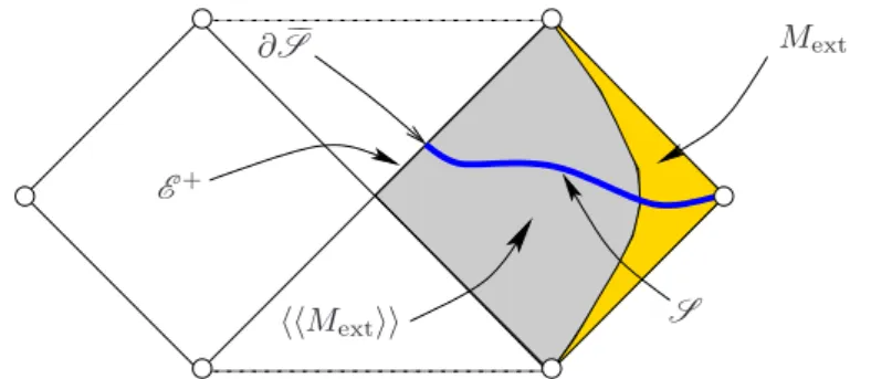
The classification theory of stationary black holes requires that the spacetime under consideration satisfies various global regularity conditions. These are captured by the following definition: Definition 2.1 Let (𝑀, g) be a spacetime containing an asymptotically-flat end, or a 𝐾𝐾-asymp-totically-flat end Sext, and let 𝑘 be a stationary Killing vector field on 𝑀 . We will say that
(𝑀, g, 𝑘) is 𝐼+-regular if𝑘 is complete, if the domain of outer communications⟨⟨𝑀ext⟩⟩ is globally
hyperbolic, and if ⟨⟨𝑀ext⟩⟩ contains a spacelike, connected, acausal hypersurface S ⊃ Sext, the
closureS of which is a topological manifold with boundary, consisting of the union of a compact set and of a finite number of asymptotic ends, such that the boundary𝜕S := S∖S is a topological manifold satisfying
𝜕S ⊂ E+:= 𝜕⟨⟨𝑀ext⟩⟩ ∩ 𝐼+(𝑀ext) , (2.23)
with𝜕S meeting every generator of E+ precisely once. (See Figure 2.)
Mext
∂S
S hhMextii
E+
Figure 2: The hypersurfaceS from the definition of 𝐼+-regularity. The “𝐼+” of the name is due to the 𝐼+ appearing in (2.23).
Some comments about the definition are in order. First, one requires completeness of the orbits of the stationary Killing vector to have an action of R on 𝑀 by isometries. Next, global hyperbolicity of the domain of outer communications is used to guarantee its simple connectedness, to make sure that the area theorem holds, and to avoid causality violations as well as certain kinds of naked singularities in⟨⟨𝑀ext⟩⟩. Further, the existence of a well-behaved spacelike hypersurface
is a prerequisite to any elliptic PDEs analysis, as is extensively needed for the problem at hand. The existence of compact cross-sections of the future event horizon prevents singularities on the future part of the boundary of the domain of outer communications, and eventually guarantees the smoothness of that boundary. The requirement Eq. (2.23) might appear somewhat unnatural, as there are perfectly well-behaved hypersurfaces in, e.g., the Schwarzschild spacetime, which do not satisfy this condition, but there arise various technical difficulties without this condition. Needless to say, all those conditions are satisfied by the Kerr–Newman and the Majumdar–Papapetrou (MP) solutions.
3
Towards a classification of stationary electrovacuum black
hole spacetimes
While the uniqueness theory for black-hole solutions of Einstein’s vacuum equations and the Einstein–Maxwell (EM) equations has seen deep successes, the complete picture is nowhere settled at the time of revising of this work. We know now that, under reasonable global conditions (see Definition 2.1), the domains of dependence of analytic, stationary, asymptotically-flat electrovac-uum black-hole spacetimes with a connected non-degenerate horizon belong to the Kerr–Newman family. The purpose of this section is to review the various steps involved in the classification of electrovacuum spacetimes (see Figure 3). In Section 5, we shall then comment on the validity of the partial results in the presence of non-linear matter fields.
For definiteness, from now on we assume that all spacetimes are 𝐼+-regular. We note that the slightly weaker global conditions spelled-out in Theorem 3.1 suffice for the analysis of static spacetimes, or for various intermediate steps of the uniqueness theory, but those weaker conditions are not known to suffice for the Uniqueness Theorem 3.3.
The main task of the uniqueness program is to show that the domains of outer communications of sufficiently regular stationary electrovacuum black-hole spacetimes are exhausted by the Kerr– Newman or the MP spacetimes.
The starting point is the smoothness of the event horizon; this is proven in [76, Theorem 4.11], drawing heavily on the results in [69].
One proves, next, that connected components of the event horizon are diffeomorphic toR × 𝑆2.
This was established in [85], taking advantage of the topological censorship theorem of Friedman, Schleich and Witt [106]; compare [141] for a previous partial result. (Related versions of the topology theorem, applying to globally-hyperbolic, not-necessarily-stationary, spacetimes, have been established by Jacobson and Venkataramani [180], and by Galloway [108, 109, 110, 112]; the strongest-to-date version, with very general asymptotic hypotheses, can be found in [73].)
3.1
Static solutions
A stationary spacetime is called static if the Killing vector 𝑘 is hypersurface-orthogonal: this means that the distribution of the hyperplanes orthogonal to 𝑘 is integrable. Equivalently,
𝑘∧ 𝑑𝑘 = 0 .
Here and elsewhere, by a common abuse of notation, we also write 𝑘 for the one-form associated with 𝑘.
The results concerning static black holes are stronger than the general stationary case, and so this case deserves separate discussion. In any case, the proof of uniqueness for stationary black holes branches out at some point and one needs to consider separately uniqueness for static configurations.
In pioneering work, Israel showed that both static vacuum [176] and electrovacuum [177] black-hole spacetimes satisfying a set of restrictive conditions are spherically symmetric. Israel’s ingenious method, based on differential identities and Stokes’ theorem, triggered a series of investigations devoted to the static uniqueness problem (see, e.g., [244, 245, 279, 281, 294]). A breakthrough was made by Bunting and Masood-ul-Alam [42], who showed how to use the positive energy theorem2
2 This theorem was first proven by Schoen and Yau [288, 289] and somewhat later, using spinor techniques, by Witten [325] (compare [265]). See [12] for a version relevant to the uniqueness problem, which allows degenerate components of the event horizon.
to exclude non-connected configurations (compare [61]).3
The annoying hypothesis of analyticity, which was implicitly assumed in the above treatments, has been removed in [72]. The issue here is to show that the Killing vector field cannot become null on the domain of outer communications. The first step to prove this is the Vishveshwara–Carter lemma (see Section 2.5.2 and [308, 43]), which shows that null orbits of static Killing vectors form a prehorizon, as defined in Section 2.5.2. To finish the proof one needs to show that prehorizons cannot occur within the d.o.c. This presents no difficulty when analyticity is assumed. Now, analyticity of stationary electrovacuum metrics is a standard property [245, 243] when the Killing vector is timelike, but timelikeness throughout the d.o.c. is not known yet at this stage of the argument. The nonexistence of prehorizons within the d.o.c. for smooth metrics requires more work, and is the main result in [72].
In the static vacuum case the remainder of the argument can be simplified by noting that there are no static solutions with degenerate horizons, which have spherical cross-sections [81]. This is not true anymore in the electrovacuum case, where an intricate argument to handle non-degenerate horizons is needed [83] (compare [284, 295, 225, 62] for previous partial results).
All this can be summarized in the following classification theorem:
Theorem 3.1 Let (𝑀, g) be an electrovacuum, four-dimensional spacetime containing a spacelike, connected, acausal hypersurfaceS , such that S is a topological manifold with boundary consisting of the union of a compact set and of a finite number of asymptotically-flat ends. Suppose that there exists on 𝑀 a complete hypersurface-orthogonal Killing vector, that the domain of outer communication ⟨⟨𝑀ext⟩⟩ is globally hyperbolic, and that 𝜕S ⊂ 𝑀 ∖ ⟨⟨𝑀ext⟩⟩. Then ⟨⟨𝑀ext⟩⟩ is
isometric to the domain of outer communications of a Reissner–Nordstr¨om or a MP spacetime.
3.2
Stationary-axisymmetric solutions
3.2.1 TopologyA second class of spacetimes where reasonably satisfactory statements can be made is provided by stationary-axisymmetric solutions. Here one assumes from the outset that, in addition to the stationary Killing vector, there exists a second Killing vector field. Assuming 𝐼+-regularity, one can invoke the positive energy theorem to show [18, 19] that some linear combination of the Killing vectors, say 𝑚, must have periodic orbits, and an axis of rotation, i.e., a two-dimensional totally-geodesic submanifold of 𝑀 on which the Killing vector 𝑚 vanishes. The description of the quotient manifold is provided by the deep mathematical results concerning actions of isometry groups of [259, 273], together with the simple-connectedness and structure theorems [76]. The bottom line is that the spacetime is the product ofR with R3from which a finite number of aligned
balls, each corresponding to a black hole, has been removed. Moreover, the 𝑈 (1) component of the group of isometries acts by rotations of R3. Equivalently, the quotient space is a half-plane
from which one has removed a finite number of disjoint half-discs centered on points lying on the boundary of the half-plane.
3.2.2 Candidate metrics
The only known 𝐼+-regular stationary and axisymmetric solutions of the Einstein–Maxwell
equa-tions are the Kerr–Newman metrics and the MP metrics. However, it should be kept in mind that candidate solutions for non-connected black-hole configurations exist:
3 Non-existence of certain static 𝑛-body configurations (possibly, but not necessarily, black holes) was estab-lished in [21, 20]). These results rely on the positive energy theorem and exclude, in particular, suitably regular configurations with a reflection symmetry across a noncompact surface, which is disjoint from the matter regions.
First, there are the multi-soliton metrics constructed using inverse scattering methods [23, 22] (compare [268]). Closely related (and possibly identical, see [148]), are the multi-Kerr solutions constructed by successive B¨acklund transformations starting from Minkowski spacetime; a special case is provided by the Neugebauer–Kramer double-Kerr solutions [198]. These are explicit solu-tions, with the metric functions being rational functions of coordinates and of many parameters. It is known that some subsets of those parameters lead to metrics, which are smooth at the axis of rotation, but one suspects that those metrics will be nakedly singular away from the axis. We will return to that question in Section 3.4.3.
Next, there are the solutions constructed by Weinstein [322], obtained from an abstract exis-tence theorem for suitable harmonic maps. The resulting metrics are smooth everywhere except perhaps at some components of the axis of rotation. It is known that some Weinstein solutions have conical singularities [319, 216, 249, 70] on the axis, but the general case remains open.
Finally, the Israel–Wilson–Perj´es (IWP) metrics [267, 179], discussed in more detail in Sec-tion 7.3, provide candidates for rotating generalizaSec-tions of the MP black holes. Those metrics are remarkable because they admit nontrivial Killing spinors. The Killing vector obtained from the Killing spinor is causal everywhere, so the horizons are necessarily non-rotating and degenerate. It has been shown in [80] that the only regular IWP metrics with a Killing vector timelike throughout the d.o.c. are the MP metrics. A strategy for a proof of timelikeness has been given in [80], but the details have yet to be provided. In any case, one expects that the only regular IWP metrics are the MP ones.
Some more information concerning candidate solutions with non-connected horizons can be found in Section 3.4.3.
3.2.3 The reduction
Returning to the classification question, the analysis continues with the circularity theorem of Papapetrou [264] and Kundt and Tr¨umper [201] (compare [43]), which asserts that, locally and away from null orbits, the metric of a vacuum or electrovacuum spacetime can be written in a 2+2 block-diagonal form.
The next key observation of Carter is that the stationary and axisymmetric EM equations can be reduced to a two-dimensional boundary value problem [45] (see Sections 6.1 and 8.2 for more details), provided that the area density of the orbits of the isometry group can be used as a global spacelike coordinate on the quotient manifold. (See also [47] and [50].) Prehorizons intersecting the d.o.c. provide one of the obstructions to this, and a heavy-duty proof that such prehorizons do not arise was given in [76]; a simpler argument has been provided in [72].
In essence, Carter’s reduction proceeds through a global manifestly–conformally-flat (“isother-mal”) coordinate system (𝜌, 𝑧) on the quotient manifold. One also needs to carefully monitor the boundary conditions satisfied by the fields of interest. The proof of existence of the (𝜌, 𝑧) coordi-nates, with sufficient control of the boundary conditions so that the uniqueness proof goes through, has been given in [76], drawing heavily on [64], assuming that all horizons are non-degenerate. A streamlined argument has been presented in [79], where the analysis has also been extended to cover configurations with degenerate components.
So, at this stage one has reduced the problem to the study of solutions of harmonic-type equations onR3
∖ A , where A is the rotation axis {𝑥 = 𝑦 = 0}, with precise boundary conditions at the axis. Moreover, the solution is supposed to be invariant under rotations. Equivalently, one has to study a set of harmonic-type equations on a half-plane with specific singularity structure on the boundary.
There exist today at least three arguments that finish the proof, to be described in the following subsections.
3.2.4 The Robinson–Mazur proof
In the vacuum case, Robinson was able to construct an amazing identity, by virtue of which the uniqueness of the Kerr metric followed [280]. The uniqueness problem with electro-magnetic fields remained open until Mazur [228] obtained a generalization of the Robinson identity in a systematic way: The Mazur identity (see also [229, 230, 48, 31, 168, 167]) is based on the observation that the EM equations in the presence of a Killing field describe a non-linear 𝜎-model with coset space 𝐺/𝐻 = 𝑆𝑈 (1, 2)/𝑆(𝑈 (1)× 𝑈(2)). The key to the success is Carter’s idea to carry out the dimensional reduction of the EM action with respect to the axial Killing field. Within this approach, the Robinson identity loses its enigmatic status – it turns out to be the explicit form of the Mazur identity for the vacuum case, 𝐺/𝐻 = 𝑆𝑈 (1, 1)/𝑈 (1).
Reduction of the EM action with respect to the time-like Killing field yields, instead, 𝐻 = 𝑆(𝑈 (1, 1)× 𝑈(1)), but the resulting equations become singular on the ergosurface, where the Killing vector becomes null.
More information on this subject is provided in Sections 7.1 and 8.4.1. 3.2.5 The Bunting–Weinstein harmonic-map argument
At about the same time, and independently of Mazur, Bunting [41] gave a proof of uniqueness of the relevant harmonic-map equations exploiting the fact that the target space for the problem at hand is negatively curved. A further systematic PDE study of the associated harmonic maps has been carried out by Weinstein: as already mentioned, Weinstein provided existence results for multi-horizon configurations, as well as uniqueness results [322].
All the uniqueness results presented above require precise asymptotic control of the harmonic map and its derivatives at the singular set A . This is an annoying technicality, as no detailed study of the behavior of the derivatives has been presented in the literature. The approach in [75, Appendix C] avoids this problem, by showing that a pointwise control of the harmonic map is enough to reach the desired conclusion.
For more information on this subject consult Section 8.4.2. 3.2.6 The Varzugin–Neugebauer–Meinel argument
The third strategy to conclude the uniqueness proof has been advocated by Varzugin [306, 307] and, independently, by Neugebauer and Meinel [251]. The idea is to exploit the properties of the linear problemassociated with the harmonic map equations, discovered by Belinski and Zakharov [23, 22] (see also [268]). This proceeds by showing that a regular black-hole solution must necessarily be one of the multi-soliton solutions constructed by the inverse-scattering methods, providing an argument for uniqueness of the Kerr solution within the class. Thus, one obtains an explicit form of the candidate metric for solutions with more components, as well as an argument for the non-existence of two-component configurations [249] (compare [70]).
3.2.7 The axisymmetric uniqueness theorem What has been said so far can be summarized as follows:
Theorem 3.2 Let (𝑀, g) be a stationary, axisymmetric asymptotically-flat, 𝐼+-regular, electrovac-uum four-dimensional spacetime. Then the domain of outer communications⟨⟨𝑀ext⟩⟩ is isometric
to one of the Weinstein solutions. In particular, if the event horizon is connected, then ⟨⟨𝑀ext⟩⟩
3.3
The no-hair theorem
3.3.1 The rigidity theoremThroughout this section we will assume that the spacetime is 𝐼+-regular, as made precise by
Definition 2.1.
To prove uniqueness of connected, analytic, non-degenerate configurations, it remains to show that every such black hole is either static or axially symmetric. The first step for this is provided by Hawking’s strong rigidity theorem (SRT) [143, 238, 60, 107], which relates the global concept of the event horizon to the independently-defined, and logically-distinct, local notion of the Killing horizon. Assuming analyticity, SRT asserts that the event horizon of a stationary black-hole spacetime is a Killing horizon. (In this terminology [151], the weak rigidity theorem is the existence, already discussed above, of prehorizons for static or stationary and axisymmetric configurations.) A Killing horizon is called non-rotating if it is generated by the stationary Killing field, and rotating otherwise. At this stage the argument branches-off, according to whether at least one of the horizons is rotating, or not.
In the rotating case, Hawking’s theorem actually provides only a second Killing vector field defined near the Killing horizon, and to continue one needs to globalize the Killing vector field, to prove that its orbits are complete, and to show that there exists a linear combination of Killing vector fields with periodic orbits and an axis of rotation. This is done in [60], assuming analyticity, drawing heavily on the results in [253, 57, 18].
The existing attempts in the literature to construct a second Killing vector field without assum-ing analyticity have only had limited success. One knows now how to construct a second Killassum-ing vector in a neighborhood of non-degenerate horizons for electrovacuum black holes [2, 174, 327], but the construction of a second Killing vector throughout the d.o.c. has only been carried out for vacuum near-Kerr non-degenerate configurations so far [3] (compare [326]).
In any case, sufficiently regular analytic stationary electro-vacuum spacetimes containing a rotating component of the event horizon are axially symmetric as well, regardless of degeneracy and connectedness assumptions (for more on this subject see Section 3.4.2). One can then finish the uniqueness proof using Theorem 3.2. Note that the last theorem requires neither analyticity nor connectedness, but leaves open the question of the existence of naked singularities in non-connected candidate solutions.
In the non-rotating case, one continues by showing [84] that the domain of outer communications contains a maximal Cauchy surface. This has been proven so far only for non-degenerate horizons, and this is the only missing step to include situations with degenerate components of the horizon. This allows one to prove the staticity theorem [302, 303], that the stationary Killing field of a non-rotating, electrovacuum black-hole spacetime is hypersurface orthogonal. (Compare [134, 136, 143, 141] for previous partial results.) One can then finish the argument using Theorem 3.1. 3.3.2 The uniqueness theorem
All this leads to the following precise statement, as proven in [76, 79] in vacuum and in [217, 79] in electrovacuum:
Theorem 3.3 Let (𝑀, g) be a stationary, asymptotically-flat, 𝐼+-regular, electrovacuum, four-dimensional analytic spacetime. If the event horizon is connected and either mean non-degenerate or rotating, then ⟨⟨𝑀ext⟩⟩ is isometric to the domain of outer communications of a Kerr–Newman
spacetime.
The structure of the proof can be summarized in the flow chart of Figure 3. This is to be compared with Figure 4, which presents in more detail the weaker hypotheses needed for various parts of the argument.
Stationary, analytic, connected, mean non-degenerate, 𝐼+-regular electrovacuum black-hole spacetime
[asymptotically time-like Killing field 𝑘𝜇]
Smoothness and topology theorems
STRONG RIGIDITY THM (1st part)
Event horizon = Killing horizon 𝐻[𝜉] [null generator Killing field 𝜉𝜇]
𝐻[𝜉] non-rotating: 𝑘𝜇𝑘𝜇|𝐻[𝜉]≡ 0 𝐻[𝜉] rotating: 𝑘𝜇𝑘𝜇|𝐻[𝜉]̸≡ 0
STATICITY THM STRONG RIGIDITY THM (2nd part)
d.o.c. static d.o.c. axisymmetric
[𝑘[𝛼∇𝛽𝑘𝛾]= 0] [∃ Killing field 𝑚𝜇]
STATICITY THM (2nd part) CIRCULARITY THM
d.o.c. static and strictly stationary d.o.c. circular [𝑘𝜇𝑘𝜇< 0] ∃ coordinates 𝑡, 𝜙: 𝑘𝜇= 𝜕𝑡and
∃ coordinate 𝑡: 𝑘𝜇
= 𝜕𝑡 is hypersurface orthogonal 𝑚𝜇= 𝜕𝜙are hypersurface orthogonal
STATIC UNIQUENESS THM CIRCULAR UNIQUENESS THM [originally by means of Israel’s thm, [originally by means of Robinson’s thm, later by the positive energy thm] later by 𝜎-model/harmonic map identities or by inverse scattering techniques]
Schwarzschild (Reissner–Nordstr¨om or MP) Kerr (Kerr–Newman) metric
Figure 3: Classification of analytic, connected, mean non-degenerate, asymptotically-flat, 𝐼+-regular, stationary electrovacuum black holes.
The hypotheses of analyticity and non-degeneracy are highly unsatisfactory, and one believes that they are not needed for the conclusion. One also believes that, in vacuum, the hypothesis of connectedness is spurious, and that all black holes with more than one component of the event horizon are singular, but no proof is available except for some special cases [216, 319, 249]. Indeed, Theorem 3.3 should be compared with the following conjecture, it being understood that both the Minkowski and the Reissner–Nordstr¨om spacetimes are members of the Kerr–Newman family: Conjecture 3.4 Let (𝑀, g) be an electrovacuum, four-dimensional spacetime containing a space-like, connected, acausal hypersurfaceS , such that S is a topological manifold with boundary, con-sisting of the union of a compact set and of a finite number of asymptotically-flat ends. Suppose that there exists on 𝑀 a complete stationary Killing vector 𝑘, that⟨⟨𝑀ext⟩⟩ is globally hyperbolic,
and that 𝜕S ⊂ 𝑀 ∖ ⟨⟨𝑀ext⟩⟩. Then ⟨⟨𝑀ext⟩⟩ is isometric to the domain of outer communications
of a Kerr–Newman or MP spacetime.
3.3.3 A uniqueness theorem for near-Kerrian smooth vacuum stationary spacetimes The existing results on rigidity without analyticity require one to assume either staticity, or a near-Kerr condition on the spacetime geometry (see Section 3.3.1), which is quantified in terms of a smallness condition of the Mars–Simon tensor [223, 293]. The results in [3] together with Theorems 3.1 – 3.2, and a version of the R´acz–Wald Theorem [107, Proposition 4.1], lead to: Theorem 3.5 Let (𝑀, g) be a stationary asymptotically-flat, 𝐼+-regular, smooth, vacuum four-dimensional spacetime. Assume that the event horizon is connected and mean non-degenerate. If the Mars–Simon tensor𝑆 and the Ernst potential E of the spacetime satisfy
∑︁
𝑖𝑗𝑘𝑙
|(1 − E)𝑆𝑖𝑗𝑘𝑙| < 𝜖
for a small enough𝜖 > 0, then ⟨⟨𝑀ext⟩⟩ is isometric to the domain of outer communications of a
Kerr spacetime.
3.4
Summary of open problems
For the convenience of the reader, we summarize here the main open problems left in the no-hair theorem.
3.4.1 Degenerate horizons
We recall that there exist no vacuum static spacetimes containing degenerate horizons with compact spherical sections [81]. On the other hand, MP [220, 262] black holes provide the only electro-vacuum static examples with non-connected degenerate horizons. See [78, 154] and references therein for a discussion of the geometry of MP black holes.
Under the remaining hypotheses of Theorem 3.3, the only step where the hypothesis of non-degeneracy enters is the proof of existence of a maximal hypersurface S in the black-hole spacetime under consideration, such that S is Cauchy for the domain of outer communications. The geometry of Cauchy surfaces in the case of degenerate horizons is well understood by now [62, 79], and has dramatically different properties when compared to the non-degenerate case. A proof of existence of maximal hypersurfaces in this case would solve the problem, but requires new insights. A key missing element is an equivalent of Bartnik’s a priori height estimate [10], established for asymptotically-flat ends, that would apply to asymptotically-cylindrical ends.
(𝑀, g) Stationary, asymptotically flat, electrovacuum, 𝐼+-regular black-hole spacetime [asymptotically time-like Killing field 𝑘; classification of isometry groups and actions]
Regularity and topology theorems
[horizons smooth/analytic with spherical sections; d.o.c. simply connected; structure theorem; nonexistence of prehorizons meeting the d.o.c.]
STRONG RIGIDITY THM (1st part)
Assume moreover that (𝑀, g) is either a) analytic, or b) vacuum and near-Kerrian with connected and mean non-degenerate event horizon (⟨𝜅⟩ ̸= 0).
Event horizon = Killing horizon 𝐻[𝜉]
𝐻[𝜉] non-rotating: g(𝑘, 𝑘)|𝐻(𝜉)≡ 0 𝐻[𝜉] rotating: g(𝑘, 𝑘)|𝐻(𝜉)̸≡ 0
If non-degenerate (𝜅 ̸= 0): ∙ Horizon essentially bifurcate ∙ Existence of maximal hypersurfaces
STATICITY THM STRONG RIGIDITY THM (2nd part)
d.o.c. static d.o.c. axisymmetric
𝑑𝑘♭∧ 𝑘♭
= 0 If (𝑀, g) analytic or near-Kerrian: ∃ periodic Killing field 𝑚 s.t. [𝑘, 𝑚] = 0 𝑀 ≈R × (︀R3∖ ∪𝑖𝐵𝑖)︀
𝜌2:= g2(𝑘, 𝑚) − g(𝑘, 𝑘)g(𝑚, 𝑚) ≥ 0 in d.o.c.
STATICITY THM (2nd part) CIRCULARITY THM
d.o.c. static and strictly stationary d.o.c. circular d.o.c. strictly stationary: g(𝑘, 𝑘) < 0 ∃ global Weyl coordinates (𝑡, 𝜙, 𝜌, 𝑧): ∃ coordinate 𝑡: 𝑘 = 𝜕𝑡 is 𝑘 = 𝜕𝑡, 𝑚 = 𝜕𝜙
hypersurface orthogonal g = −𝜌2𝑒2𝜆𝑑𝑡2+ 𝑒−2𝜆
(𝑑𝜙 − 𝑣𝑑𝑡)2+ 𝑒2 𝑢(𝑑𝜌2+ 𝑑𝑧2)
g = −𝑉2𝑑𝑡2+ 𝛾𝑖𝑗𝑑𝑥𝑖𝑑𝑥𝑗 (with controlled asymptotic behavior)
STATIC UNIQUENESS THM CIRCULAR UNIQUENESS THM ∙ originally by means of Israel’s thm, ∙ originally by means of Robinson’s thm, later by the positive energy thm later by 𝜎-model/harmonic map identities ∙ No analyticity, degeneracy or or by inverse scattering techniques connectedness needed ∙ multi-black holes?
Reissner–Nordstr¨om or MP Kerr–Newman metric
3.4.2 Rigidity without analyticity
Analyticity enters the current argument at two places: First, one needs to construct the second Killing vector near the horizon. This can be done by first constructing a candidate at the horizon, and then using analyticity to extend the candidate to a neighborhood of the horizon. Next, the Killing vector has to be extended to the whole domain of outer communications. This can be done using analyticity and a theorem by Nomizu [253], together with the fact that 𝐼+-regular domains
of outer communications are simply connected. Finally, analyticity can be used to provide a simple argument that prehorizons do not intersect⟨⟨𝑀ext⟩⟩ (but this is not critical, as a proof is available
now within the smooth category of metrics [72]).
A partially-successful strategy to remove the analyticity condition has been invented by Alex-akis, Ionescu and Klainerman in [2]. Their argument applies to non-degenerate near-Kerrian configurations, but the general case remains open.
The key to the approach in [2] is a unique continuation theorem near bifurcate Killing horizons proven in [174], which implies the existence of a second Killing vector field, say 𝑚, in a neigh-borhood of the horizon. One then needs to prove that 𝑚 extends to the whole domain of outer communications. This is established via another unique continuation theorem [175] with specific convexity conditions. These lead to non-trivial restrictions, and so far the argument has only been shown to apply to near-Kerrian configurations.
A unique continuation theorem across more general timelike surfaces would be needed to obtain the result without smallness restrictions.
It follows from what has been said in [72] that the boundary of the set where two Killing vector fields are defined cannot become null within a domain of outer communications; this fact might be helpful in solving the full problem.
3.4.3 Many components?
The only known examples of singularity-free stationary electrovacuum black holes with more than one component are provided by the MP family. (Axisymmetric MP solutions are possible, but MP metrics only have one Killing vector in general.) It has been suspected for a very long time that these are the only such solutions, and that there are thus no such vacuum configurations. This should be contrasted with the five-dimensional case, where the Black Saturn solutions of Elvang and Figueras [97] (compare [71, 305]) provide non-trivial two-component examples.
It might be convenient to summarize the general facts known about four-dimensional multi-component solutions.4 In case of doubts, 𝐼+-regularity should be assumed.
We start by noting that the static solutions, whether connected or not, have already been covered in Section 3.1.
A multi-component electro-vacuum configuration with all components degenerate and non-rotating would be, by what has been said, static, but then no such solutions exist (all components of an MP black hole are degenerate). On the other hand, the question of existence of a multi– black-hole configuration with components of mixed type, none of which rotates, is open; what’s missing is the proof of existence of maximal hypersurfaces in such a case. Neither axisymmetry nor staticity is known for such configurations.
Analytic multi–black-hole solutions with at least one rotating component are necessarily ax-isymmetric; this leads one to study the corresponding harmonic-map equations, with candidate solutions provided by Weinstein or by inverse scattering techniques [198, 322, 23, 22]. The Wein-stein solutions have no singularities away from the axes, but they are not known in
4 Here we are interested in stationary multi–black-hole configurations; nonexistence of some suitably regular stationary 𝑛-body configurations was established, under different symmetry conditions, in [20, 21].
explicit form, which makes difficult the analysis of their behavior on the axis of rotation. The multi–black-hole metrics constructed by multi-soliton superpositions or by B¨acklund transforma-tion techniques are obtained as ratransforma-tional functransforma-tions with several parameters, with explicit constraints on the parameters that lead to a regular axis [222], but the analysis of the zeros of their denom-inators has proved intractable so far. It is perplexing that the five dimensional solutions, which are constructed by similar methods [268], can be completely analyzed with some effort and lead to regular solutions for some choices of parameters, but the four-dimensional case remains to be understood.
In any case, according to Varzugin [306, 307] and, independently, to Neugebauer and Meinel [251] (a more detailed exposition can be found in [249, 147]), the multi-soliton solutions provide the only candidates for stationary axisymmetric electrovacuum solutions. A breakthrough in the understanding of vacuum two-component configurations has been made by Hennig and Neuge-bauer [147, 249], based on the area-angular momentum inequalities of Ansorg, Cederbaum and Hennig [145] as follows: Hennig and Neugebauer exclude many of the solutions by verifying that they have negative total ADM mass. Next, configurations where two horizons have vanishing surface gravity are shown to have zeros in the denominators of some geometric invariants. For the remaining ones, the authors impose a non-degeneracy condition introduced by Booth and Fairhurst [25]: a black hole is said to be sub-extremal if any neighborhood of the event horizon contains trapped surfaces. The key of the analysis is the angular momentum - area inequality of Hennig, Ansorg, and Cederbaum [145], that on every sub-extremal component of the horizon it holds that
8𝜋|𝐽| < 𝐴 , (3.1) where 𝐽 is the Komar angular-momentum and 𝐴 the area of a section. (It is shown in [7] and [146, Appendix] that 𝜅 = 0 leads to equality in (3.1) under conditions relevant to the problem at hand.) Hennig and Neugebauer show that all remaining candidate solutions violate the inequality; this is their precise non-existence statement.
The problem with the argument so far is the lack of justification of the sub-extremality con-dition. Fortunately, this condition can be avoided altogether using ideas of [88] concerning the inequality (3.1) and appealing to the results in [96, 6, 73] concerning marginally–outer-trapped surfaces (MOTS): Using existence results of weakly stable MOTS together with various aspects of the candidate Weyl metrics, one can adapt the argument of [145] to show [70] that the area inequality (3.1), with “less than” there replaced by “less than or equal to”, would hold for those components of the horizon, which have non-zero surface gravity, assuming an 𝐼+-regular metric of
the Weyl form, if any existed. The calculations of Hennig and Neugebauer [249] together with a contradiction argument lead then to
Theorem 3.6 𝐼+-regular two-Kerr black holes do not exist. The case of more than two horizons is widely open.
4
Classification of stationary toroidal Kaluza–Klein black
holes
In this work we are mostly interested in uniqueness results for four-dimensional black holes. This leads us naturally to consider those vacuum Kaluza–Klein spacetimes with enough symmetries to lead to dimensional spacetimes after dimensional reduction, providing henceforth four-dimensional black holes. It is convenient to start with a very short overview of the subject; the reader is referred to [101, 172] and references therein for more information. Standard examples of Kaluza–Klein black holes are provided by the Schwarzschild metric multiplied by any spatially flat homogeneous space (e.g., a torus). Non-trivial examples can be found in [272, 211]; see also [200, 172] and reference therein.
4.1
Black holes in higher dimensions
The study of spacetimes with dimension greater then four is almost as old as general relativity it-self [183, 195]. Concerning black holes, while in dimension four all explicitly-known asymptomatically-flat and regular solutions of the vacuum Einstein equations are exhausted by the Kerr family, in spacetime dimension five the landscape of known solutions is richer. The following 𝐼+-regular,
stationary, asymptotically-flat, vacuum solutions are known in closed form: the Myers–Perry black holes, which are higher-dimensional generalizations of the Kerr metric with spherical-horizon topology [246]; the celebrated Emparan–Reall black rings with 𝑆2× 𝑆1 horizon topology [99];
the Pomeransky–Senkov black rings generalizing the previous by allowing for a second angular-momentum parameter [269]; and the “Black Saturn” solutions discovered by Elvang and Figueras, which provide examples of regular multi-component black holes where a spherical horizon is sur-rounded by a black ring [97].5
Inspection of the basic features of these solutions challenges any naive attempt to generalize the classification scheme developed for spacetime dimension four: One can find black rings and Myers– Perry black holes with the same mass and angular momentum, which must necessarily fail to be isometric since the horizon topologies do not coincide. In fact there are non-isometric black rings with the same Poincar´e charges; consequently a classification in terms of mass, angular momenta and horizon topology also fails. Moreover, the Black Saturns provide examples of regular vacuum multi–black-hole solutions, which are widely believed not to exist in dimension four; interestingly, there exist Black Saturns with vanishing total angular momentum, a feature that presumably distinguishes the Schwarzschild metric in four dimensions.
Nonetheless, results concerning 4-dimensional black holes either generalize or serve as inspi-ration in higher dimensions. This is true for landmark results concerning black-hole uniqueness and, in fact, classification schemes exist for classes of higher dimensional black-hole spacetimes, which mimic the symmetry properties of the “static or axisymmetric” alternative, upon which the uniqueness theory in four-dimensions is built.
For instance, staticity of 𝐼+-regular, vacuum, asymptotically-flat, non-rotating, non-degenerate
black holes remains true in higher dimensions6. Also, Theorem 3.1 remains valid for vacuum
space-times of dimension 𝑛 + 1, 𝑛≥ 3, whenever the positive energy theorem applies to an appropriate doubling of S (see [72], Section 3.1 and references therein). Moreover, the discussion in Section 3.1 together with the results in [282, 283] suggest that an analogous generalization to electrovacuum spacetimes exists, which would lead to uniqueness of the higher-dimensional Reissner–Nordstr¨om metrics within the class of static solutions of the Einstein–Maxwell equations, for all 𝑛 ≥ 3 (see also [101, Section 8.2], [173] and references therein).
5Studies of regularity and causal structure of black rings and Saturns can be found in [82, 67, 68, 305, 71]. 6 It should be noted that, although formulated for 4-dimensional spacetimes, the results in [84] remain valid without changes in higher-dimensional spacetimes.