How important is adapting regional climatic projections to the local environment? A procedure for microclimatic corrections makes the difference for crop growth in a virtual experiment

(1)

141 4th European Agroforestry Conference Agroforestry as Sustainable Land Use

HOW IMPORTANT IS ADAPTING REGIONAL CLIMATIC

PROJECTIONS TO THE LOCAL ENVIRONMENT? A

PROCEDURE FOR MICROCLIMATIC CORRECTIONS

MAKES THE DIFFERENCE FOR CROP GROWTH IN A

VIRTUAL EXPERIMENT

Reyes F1_{*, Gosme M}1_{, Blanchet G}1_{, Dupraz C}1

(1) INRA, System, University of Montpellier, Montpellier, France *Corresponding author: reyes.francesco@protonmail.com

Abstract

Climatic conditions drive plant metabolism and growth and their projections are used as drivers in modelling experiments for the prediction of crop yields. However, these are generally issued at regional scale, and do not consider microclimatic variations. In this study we question the impact of taking into account microclimate adjustments on simulated crop yield. A procedure for the correction of temperature and humidity to the local microclimate is proposed and applied on climatic predictions for a site, resulting in modifications of about 2% in mean daily relative -based agroforestry model, for the pure crop and in the alley-cropping system, using both climatic series. Predicted crop yield differed by up to 58% in individual years and overall by 22% (CV RMSE) across climatic series. A significant trend in crop yield disappeared after corrections. This study highlights the importance of taking into account microclimatic corrections when using climatic projections to predict crop growth on realistic sites.

Keywords: microclimate; model; Hi-sAFe; temperature; climatic series; alleycropping

Introduction

Temperature is the primary driver of plant metabolic processes and phenology, and its variations lead the plant closer or further from its optimal growth conditions. As such, microclimatic variation might have important impact on crop yields, no matter if they are the result of spatial heterogeneity or temporal dynamics, such as in climate change. Climate change projections at regional scale are important tools to develop adaptation strategies in agriculture (e.g. development of new varieties). Conversely, knowledge of the microclimatic conditions at local scale is essential in parcel design (e.g. species selection), especially in areas with high morphological heterogeneity. Given the long lifetime of the trees, agroforestry parcel design might need to take into account both the temporal scale relevant in climate change projections and the microclimatic effects of a particular location on the plants. In this regard, we question the need to adapt regional scale climatic projections to the microclimatic conditions present in the specific site, for which a virtual experiment is performed. First, we present a procedure to adapt climatic series, provided at regional scale, to specific field sites. Then, the impact of this procedure is assessed by adjusting a climatic projection issued at regional scale to the microclimate of a given site. Both climatic series are used to drive crop development in monoculture and alley-cropping in a processed-based crop model. Crop growth results are compared and the impact of the different climatic series is discussed.

(2)

Materials and methods Data extraction

We used the the Clipick website (Palma 2017) to extract three climatic projections issued by two Global Climate Models (HadCM3Q0 and RACMO22E-KNMI models, Assessment Reports 4 and 5 respectively, of the Intergovernmental Panel on Climate Change) and downscaled via Regional Climate Models. The climatic series were extracted for an experimental plot present in Restinclieres (Montpellier, Southern France, lat: 43.7, long: 3.5, 62m ASL). Two of them represented historical (hist scenario, years 1951 to 2005) and predicted (RCP8.5 scenario, years 2006 to 2070) climatic conditions according to the RACMO22E-KNMI Global Climate Model (Assessment Report 5, IPPC). These were later adjusted to the local microclimate, and used in a virtual experiment to drive crop growth. The third series represented the whole period from 1951 to 2070, according to the HadCM3Q0 Global Climate Model, A1B scenario (Riahi et al. 2011; Palma 2017) (Assessment Report 4, IPPC) and was used to indirectly estimate two meteorological variables (minimum and maximum relative humidity) necessary to run simulations with our crop growth model (see Simulations), but missing in the hist and RCP 8.5. All series had a daily time resolution. Spatial resolution was of 11 km for hist and RCP 8.5, and of 25km for A1B (Palma 2017).

Data adjustments: temperature and relative humidity

The area surrounding the study site is characterized by a high morphological heterogeneity, suggesting that relevant temperature (T) and relative humidity (RH) differences could be present between the retrieved datasets at regional scale (hist and RCP 8.5) and measurements performed in the field (data available from year 1995 to 2014). Beside them, also other meteorological variables, such as the incoming radiation and precipitation, might be influenced by local microclimate but, we suppose, at a relatively larger spatial scale, and are not included in the presented procedure for meteorological corrections.

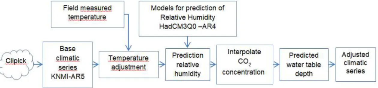
First step of the proposed method (Figure 1) is the correction of maximum (Tmax) and minimum (Tmin) daily temperatures, and is based on the periods of overlap between field measured and downloaded data series. For each period of overlap between measured and projected data:

i) the mean monthly differences (biases) between Tmin and Tmax of the two data series were calculated;

ii) the calculated biases were used to adjust Tmin and Tmax of the projected daily temperatures by subtraction.

Corrections in RH were then necessary in order to: i) take into account temperature adjustment and ii) provide maximum and minimum RH (RHmin and RHmax), available in A1B, but not in RCP 8.5 (in RCP 8.5 only the mean RH is provided). Therefore, mean daily RH was computed in A1B as the mean of max and min RH. Two multiple linear models were then built to predict RHmin and RHmax from mean RH, Tmax, Tmin, precipitation and global shortwave radiation on A1B. The same models were then used to predict RHmin and RHmax for the RCP 8.5 temperature adjusted data series.

Completion of climatic series: CO2 and water table depth

In order to be able to run simulations with the Hi-sAFe model, carbon dioxide concentration and the depth of the water table needed to be added to dataset. Carbon dioxide concentration were added by linear interpolation between historical and predicted values in years 1950 and 2100 (Meinshausen et al. 2011), without taking into account seasonal variations. An empirical model calibrated on the same parcel (Talbot 2011) was then used to predict the fluctuation in the depth of the water table from the climatic data.

Simulations

In order to estimate the impact of the climatic adjustments on simulated crop yields for an alley-cropping (AF) and a monoculture (A) parcel, we simulated crop growth under both the base and the adjusted climatic series, for the historical period between years 1951-1990. Simulations

(3)

were run with the Hi-sAFe model, a process based, purely deterministic, spatially explicit agroforestry model. This represents the three dimensional development of an alley-cropping system including tree and/or crop species, their synchronous use light, water and nitrogen resources (Talbot 2011).

Parcel description

The simulated AF parcel included a 9 m deep, mixed clay-limestone soil, with a high maximum water holding capacity (about 3400 mm) and a water table fluctuating between 6.8 and 1.3 m below ground surface (mean -4.88 +- 1.05 m). Hybrid walnut (Juglans nigra) trees were spaced 9 meters along the tree row and 13 meters between tree rows in alley-cropping parcels, while durum-allur-wheat was sown (at DOY 300) in the alley. The A parcel was described and managed identically, but did not contain trees.

Figure 1: Adjustment and completion of climatic series.

Results and discussion

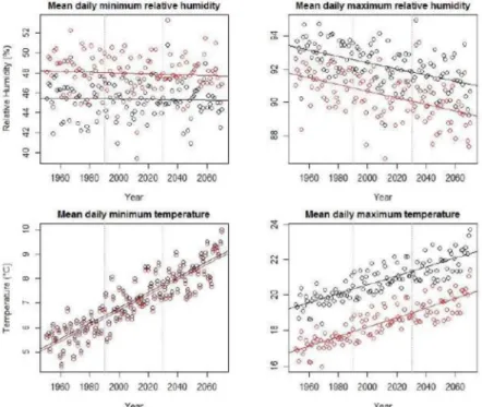
min and Tmax across the projected period (Figure 2). Differences between the base and the adjusted mean daily temperatures were negligible for Tmin max. The linear models used to estimate min and max mean daily RH were quite robust (R2RHmin = 0.90, R2RHmax = 0.85). The predicted mean daily RHmin remained approximately stable across time, while RHmax decreased by 2.5%. Differences between the base and adjusted RH, were of about 2.5% for RHmin and of about 2% in RHmax.

(4)

Figure 2: Base (red) and adjusted (black) climatic series with linear models of their trend lines. Vertical lines split the climatic series in three periods of 40 years each. Crop growth simulation was run during the first period.

Mean crop yield was, as reported in other agroforestry studies on wheat, lower in AF than in A (13%) (Dufour et al. 2013). Mean yield obtained in the adjusted series was higher (12%) than in the base series (Table 1). Crop yield variability in AF was also lower than in A, especially during the second half of each simulation, supposedly as a result of the milder microclimate established under mature trees (Table 1).

The relative difference in crop yields among climatic series (expressed by the coefficient of variation of the root mean squared error, CV RMSE) was about the same in A and AF (22%, Table 1). This suggests that the impact of the climatic corrections on crop yield was similar for both agricultural systems, when considering entire simulations. Also the maximum difference in mean crop yield was similar across parcel types (55% in A, 58% in AF).

Crop yield was generally lower or equal in the base series in respect to the adjusted one, especially during the first twenty years of growth (Figure 3). Yield significantly increased in A across the base series, following the increase in mean daily Tmax, while not in the adjusted one, which was characterized by higher mean maximum daily temperatures.

These considerations suggest that the crop might have performed better over time under the base series thanks to the temperature entering more often the range of optimal crop growth conditions. Once in this range of temperatures, further increase, corresponding to the second half of the simulation with the base series (effect of global warming) and to the simulations with the adjusted series (effect of microclimatic correction), would not contribute any further in increasing crop yields. This hypothesis is also supported by the more constant crop yield variability obtained in A with the adjusted in respect to the base series, suggesting that the additional increases in temperature occurring in this simulation do not anymore systematically affect crop yield (Table 1). As such, using the climatic series after microclimatic corrections had a considerable impact both on the magnitude of the resulting crop yield and on the direction of the simulated trends in crop yield (the significant positive relationship between yields and time in A disappears after correction (Figure 3).

(5)

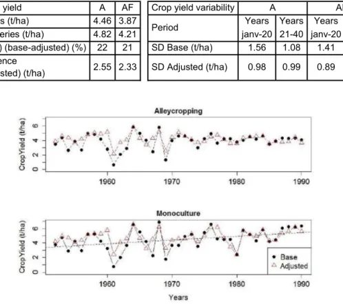
Table 1: Mean crop yield and crop yield variability (SD: standard deviation) across agricultural systems (A: pure culture, AF: alley-cropping) and data series.

Mean crop yield A AF Crop yield variability A AF

Base series (t/ha) 4.46 3.87

Period Years Years Years Years

Adjusted series (t/ha) 4.82 4.21 janv-20 21-40 janv-20 21-40

CV(RMSE) (base-adjusted) (%) 22 21 SD Base (t/ha) 1.56 1.08 1.41 0.44

Max difference

(base-adjusted) (t/ha) 2.55 2.33 SD Adjusted (t/ha) 0.98 0.99 0.89 0.4

Figure 3: Simulated crop yield in alley-cropping and pure culture, with base and adjusted climatic series. A significative (p <0.01) linear model between crop yield and time is showed by a trend line for the base simulation in pure culture.

Our case study showed that even modest differences between a climatic projection and field mean daily Tmax, 2 to 2.5% in min and max mean daily RH) can result in relevant changes in simulated yields and their interannual variability, highlighting the importance of taking into account microclimatic differences when using climatic projections for virtual experiments. We proposed an automatized and fast procedure to adjust climatic projections from the regional to the parcel scale, accounting for microclimatic variations in temperature and relative humidity, that can be relevant to better adapt crop gwoth simulations to specific sites. When used in combination with a tool such as Clipick, this becomes applicable for any site reasonably close to a meteorological station.

References

Dufour L, Metay A, Talbot G, Dupraz C (2013) Assessing Light Competition for Cereal Production in Temperate Agroforestry Systems using Experimentation and Crop Modelling. J Agron Crop Sci 199: 217 227.

Meinshausen M, Smith SJ, Calvin K, Daniel JS, Kainuma MLT, Lamarque JF, Matsumoto K, Montzka SA, Raper SCB, Riahi K, ThomsonA, Velders GJM, van Vuuren DPP (2011) The RCP greenhouse gas concentrations and their extensions from 1765 to 2300. Climatic Change 109: 213 241.

Palma JHN (2017) CliPick Climate change web picker. A tool bridging daily climate needs in process based modelling in forestry and agriculture. Forest Syst 26: eRC01.

Riahi K, Rao S, Krey V, Cho C, Chirkov V, Fischer G, Kindermann G, Nakicenovic N, Rafaj P (2011) RCP 8.5 A scenario of comparatively high greenhouse gas emissions. Climatic Change 109: 33 57.